| Issue |
A&A
Volume 505, Number 2, October II 2009
|
|
|---|---|---|
| Page(s) | 763 - 770 | |
| Section | The Sun | |
| DOI | https://doi.org/10.1051/0004-6361/200811484 | |
| Published online | 15 June 2009 | |
Acoustic oscillations in the field-free, gravitationally stratified cavities under solar bipolar magnetic canopies
D. Kuridze1,2 - T. V. Zaqarashvili2 - B. M. Shergelashvili1,2,3 - S. Poedts1
1 - Center for Plasma Astrophysics, K.U. Leuven, 200 B, 3001 Leuven, Belgium
2 -
Georgian National Astrophysical Observatory at the Faculty of Physics and
Mathematics, I. Chavchavadze State University, Al. Kazbegi ave. 2a,
0160 Tbilisi, Georgia
3 -
Institute for Theoretical Physics, K.U. Leuven, Celestijnenlaan 200 D, 3001 Leuven, Belgium
Received 8 December 2008 / Accepted 28 April 2009
Abstract
Aims. The main goal here is to study the dynamics of the gravitationally stratified, field-free cavities in the solar atmosphere, located under small-scale, cylindrical magnetic canopies, in response to explosive events in the lower-lying regions (due to granulation, small-scale magnetic reconnection, etc.).
Methods. We derive the two-dimensional Klein-Gordon equation for isothermal density perturbations in cylindrical coordinates. The equation is first solved by a standard normal mode analysis to obtain the free oscillation spectrum of the cavity. Then, the equation is solved in the case of impulsive forcing associated to a pressure pulse specified in the lower lying regions.
Results. The normal mode analysis shows that the entire cylindrical cavity of granular dimensions tends to oscillate with frequencies of 5-8 mHz and also with the atmospheric cut-off frequency. Furthermore, the passage of a pressure pulse, excited in the convection zone, sets up a wake in the cavity oscillating with the same cut-off frequency. The wake oscillations can resonate with the free oscillation modes, which leads to an enhanced observed oscillation power.
Conclusions. The resonant oscillations of these cavities explain the observed power halos near magnetic network cores and active regions.
Key words: Sun: photosphere - Sun: oscillations
1 Introduction
Observations show a high spectral power of oscillations
(![]() mHz) in the vicinity of active regions. The observed
velocity power maps are sometimes referred to as ``photospheric power
halos'' (Braun et al. 1992; Brown et al. 1992; Hindman & Brown 1998;
Jain & Haber 2002; Muglach et al. 2005; Moretti et al. 2007;
Nagashima et al. 2007; Hanasoge 2008). The power enhancement is only
observed in the Doppler velocity power maps and not in continuum
intensity (Hindman & Brown 1998; Jain & Haber 2002; Muglach et al.
2005; Nagashima et al. 2007). The enhanced power spectra peak at the
period of
mHz) in the vicinity of active regions. The observed
velocity power maps are sometimes referred to as ``photospheric power
halos'' (Braun et al. 1992; Brown et al. 1992; Hindman & Brown 1998;
Jain & Haber 2002; Muglach et al. 2005; Moretti et al. 2007;
Nagashima et al. 2007; Hanasoge 2008). The power enhancement is only
observed in the Doppler velocity power maps and not in continuum
intensity (Hindman & Brown 1998; Jain & Haber 2002; Muglach et al.
2005; Nagashima et al. 2007). The enhanced power spectra peak at the
period of ![]() 3 min.
3 min.
In addition, observations show that the chromospheric active regions and magnetic network elements are surrounded by ``magnetic shadows'', which lack oscillatory power in the higher frequency range (McIntosh & Judge 2001; Krijger et al. 2001; Vecchio et al. 2007). From the observations it seems reasonable to conclude that both the photospheric power halos and the chromospheric magnetic shadows reflect the same physical process.
In our previous paper (Kuridze et al. 2008), we proposed an explanation of the photospheric power halos as the effect of a magnetic canopy on the wave dynamics. We showed that the field-free cavity regions under the magnetic canopy can trap high-frequency acoustic oscillations, leading to the observed increased high-frequency power in the photosphere, while the lower-frequency oscillations are channeled upwards in the form of magneto-acoustic waves (Erdélyi et al. 2007; Srivastava et al. 2008). However, those calculations have been performed without taking the gravitational stratification into account, which is important at the photospheric level.
In the present paper, we study acoustic oscillations in the stratified, cylindrical field-free cavity regions under the magnetic canopy as a possible explanation of the power-halo phenomenon. There are various analytical and numerical investigations of the acoustic wave propagation in isothermal stratified atmospheres (e.g., Lamb 1908; Rae & Roberts 1982; Fleck & Schmitz 1991; Kalkofen et al. 1993; Sutmann et al. 1998; Roberts 2004). However, almost all these calculations involve simple 1D models (for vertically propagating acoustic waves), because 2D and 3D models necessarily include internal gravity waves, which considerably complicates the analysis. To avoid further complications from the gravity waves, it is possible, however, to only consider isothermal propagation, which automatically neglects gravity waves. This enables us to study the 2D propagation of only isothermal acoustic waves or pulses in a stratified atmosphere. Here, we study normal isothermal acoustic oscillations and the propagation of acoustic pulses in a cylindrical field-free cavity by solving the 2D Klein-Gordon equation in cylindrical geometry. Unlike the 1D case, the two-dimensional solution allows us to investigate the variation in the density/velocity perturbation amplitude in the azimuthal direction. First, we use a standard normal mode analysis to study the spectrum of possible acoustic oscillations in the cavity region. Then, we solve the Klein-Gordon equation with impulsive forcing in the photospheric region.
The outline of the paper is as follows. In Sect. 2 we present the basic hydrodynamic equations for the problem of the propagation of acoustic waves in a stratified cavity medium. Section 3 describes the normal mode approach and the resulting oscillation spectrum in the cavity. In Sects. 5 and 6 we analyze the response of the cavity region to a pressure pulse. The results obtained are discussed in Sect. 7.
2 The wave equation
We use the ideal hydrodynamic equations for a gravitationally stratified
field-free cavity:
 |
(1) |
 |
(2) |
 |
(3) |
where
The considered acoustic cavity under the cylindrical magnetic canopy
has a semicircular form (Fig. 1). Therefore, it is convenient to
consider Eqs. (1-3) in a cylindrical coordinate system. For
simplicity, we study the 2D case, i.e. perturbations polarized in
the ![]() plane, where r is the radial coordinate and
plane, where r is the radial coordinate and ![]() is the azimuthal angle.
is the azimuthal angle.
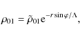
In this cylindrical (or polar) coordinate system, the equilibrium
pressure and density are related as
 |
(4) |
 |
(5) |
where p01,

are the r- and
![\begin{figure}
\par\includegraphics[width=7cm,clip]{11484fg1.eps}
\end{figure}](/articles/aa/full_html/2009/38/aa11484-08/img22.png) |
Figure 1: Simple schematic picture of small-scale magnetic canopy overlying a field-free cavity with gravitational stratification, g. |
| Open with DEXTER | |
Equations (4, 5) then easily lead to the equilibrium values of the
pressure and the density in the cavity:
 |
(6) |
 |
(7) |
where
 |
(8) |
is the pressure-scale height. The atmosphere is considered to be isothermal. Therefore, this pressure scale height is constant.
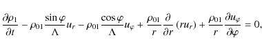
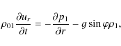
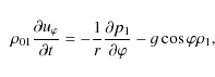
In the considered cylindrical (polar) coordinate system, the
linearized hydrodynamic equations for adiabatic fluctuations can be
written as
 |
(9) |
 |
(10) |
 |
(11) |
 |
(12) |
where
 |
(13) |
These equations describe the acoustic and internal gravity waves propagating in a stratified atmosphere. In principle, the cavity under a magnetic canopy may trap both types of waves. Unfortunately, the simultaneous consideration of both wave types is very complicated, especially from an analytical point of view. However, by adopting specific approximations, we can consider each of the wave types separately. The limit of incompressibility, e.g., neglects the acoustic branch so only gravity waves remain in this case. On the other hand, the limit of isothermal propagation neglects the gravity branch of the spectrum, and in this case, only the acoustic branch remains. The latter limit means that the temperature exchange is so rapid that any temperature fluctuation in the perturbations is zero. This is achieved when
We use the approximation/limit of isothermal propagation in the remaining part of this paper. For
isothermal perturbations, Eqs. (9-12) lead to the following wave equation:
 |
+ |  |
|
| + |  |
(14) |
Equation (14) can be written in a more convenient form by using the following transformation:
 |
(15) |
where the parameter
By substituting Eq. (15) into Eq. (14) we obtain
| |
+ |  |
|
| - | (16) |
from which we find the following condition on
 |
(17) |
or
 |
(18) |
Using this condition, we obtain
![\begin{displaymath}\frac{\partial ^{2}\tilde{\rho }_{1}}{\partial r^{2}}+{1\over...
... }_{1}}{\partial
t^{2}}+\omega^2_{ac}\tilde{\rho_1}\right ]=0,
\end{displaymath}](/articles/aa/full_html/2009/38/aa11484-08/img43.png) |
(19) |
where
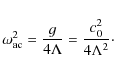 |
(20) |
Equation (19) is the Klein-Gordon equation in cylindrical/polar coordinates. This equation governs the isothermal propagation of acoustic waves (and pulses) in the considered gravitationally stratified medium. The very dynamic convective layer located under the cavity can excite quasi-harmonic wave trains, as well as acoustic pulses. Clearly, the cavity will respond in different ways to these different types of perturbations. We study two different responses of the cavity to such different perturbations from below. First, we consider the cavity as a resonator for acoustic waves and, using the standard normal mode approach, we study the spectrum of possible wave harmonics trapped in the canopy. Next, we consider the propagation of a pressure pulse, which can be caused in the lower regions by the eruption of new granular cells or by some small-scale magnetic reconnection processes.
3 Normal mode analysis
A standard Fourier analysis of Eq. (19) with respect to time leads
to the equation:
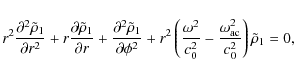 |
(21) |

which gives

We consider the solution of Eq. (21) in three different cases depending on the size of the circular frequency
When
![]() ,
Eq. (21) leads to the Laplace
equation in cylindrical coordinates. The solution of this equation
inside the canopy (i.e. inside the semicircle
,
Eq. (21) leads to the Laplace
equation in cylindrical coordinates. The solution of this equation
inside the canopy (i.e. inside the semicircle
![]() ,
where
,
where ![]() is the cavity/canopy boundary (see Fig. 1)) with the condition
is the cavity/canopy boundary (see Fig. 1)) with the condition
![]() (i.e. a Dirichlet condition)
along the boundary is given by (Morse & Feshbach 1953)
(i.e. a Dirichlet condition)
along the boundary is given by (Morse & Feshbach 1953)
![\begin{displaymath}{\tilde\rho}_1=\sum_{m=0}^{\infty}[A_m\cos(m\phi)+B_m\sin(m\phi)]\left({r\over
r_{\rm c}}\right)^m,
\end{displaymath}](/articles/aa/full_html/2009/38/aa11484-08/img53.png) |
(22) |
where
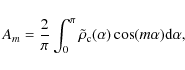 |
(23) |
and
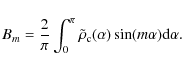 |
(24) |
This means that one of the free oscillation modes in the cavity oscillates at the cut-off frequency for any m (which plays the role of azimuthal wave number). For the photospheric sound speed of 7.5 km s-1, the acoustic cut-off frequency is on the order of 0.031 s-1 with a corresponding period of
In the case
![]() ,
Eq. (21), again after a Fourier
analysis with respect to the azimuthal direction and with azimuthal
wave number m, transforms to a Bessel equation with the general solution
,
Eq. (21), again after a Fourier
analysis with respect to the azimuthal direction and with azimuthal
wave number m, transforms to a Bessel equation with the general solution
| (25) |
where Jm and Ym are the bessel functions of the first and second kinds, respectively, and c1 and c2 are arbitrary constants.
When
![]() ,
then a similar Fourier analysis
transforms Eq. (21) to the modified Bessel equation, with the
general solution
,
then a similar Fourier analysis
transforms Eq. (21) to the modified Bessel equation, with the
general solution
| (26) |
where Im and Km are the modified Bessel functions of the first and second kinds, respectively, and c3 and c4 are arbitrary constants. The density perturbations must be finite at r=0, which yields the condition c2=c4=0. We also need a second condition at the upper boundary of the cavity in order to find a unique solution for Eq. (21). The correct approach is to find an analytical solution to the magnetohydrodynamic equations in the overlying magnetic canopy region and then merge it with the solution (25) at the canopy/cavity interface (
| (27) |
| (28) |
The first condition gives oscillatory solutions (oscillating with respect to the r-coordinate), while the second is only satisfied when c3=0. Therefore, Eq. (28) yields the trivial solution of Eq. (21), and in the following we concentrate on the oscillatory solution connected with only condition (27). The spectrum of acoustic oscillations in the cavity can then be deduced from the zeros of the solution Jm(z), which (as it is known from the theory of Bessel functions) are all real when
![\begin{figure}
\par\includegraphics[width=8.9cm,clip]{11484fg2}
\end{figure}](/articles/aa/full_html/2009/38/aa11484-08/img64.png) |
Figure 2:
The oscillation frequency, |
| Open with DEXTER | |
Figure 2 shows the dependence of the frequencies of the acoustic
oscillations on the cavity radius, ![]() ,
for the first zero of
Jm(z) for the m=1,2,3 harmonics. It is evident from this figure
that the frequency decreases with increasing
,
for the first zero of
Jm(z) for the m=1,2,3 harmonics. It is evident from this figure
that the frequency decreases with increasing ![]() ,
as can be
expected from physical considerations. This means that these
cavities, with typical granular radii
,
as can be
expected from physical considerations. This means that these
cavities, with typical granular radii
![]() km, support
oscillations with frequencies in the range 0.07-
km, support
oscillations with frequencies in the range 0.07-![]() s-1(i.e. with periods of
s-1(i.e. with periods of ![]() min). For considerably large cavity
radii, the frequencies of all the harmonics tend to the cut-off
value.
min). For considerably large cavity
radii, the frequencies of all the harmonics tend to the cut-off
value.
It seems that cylindrical cavities support higher frequency
oscillations than typical quiet Sun regions, because in cylindrical
cavities, the oscillations are partly along the ![]() -direction due
to the small k1 term for the first zero of Bessel function in
Eq. (27), which prevents their leakage upwards and leads to their
trapping in the cavities. On the other hand, the regions without
overlying canopies (e.g., nonmagnetic quiet Sun regions outside the
network cores) cannot trap the high frequency oscillations, because
they may propagate upwards. Therefore, it is expected that the
high-frequency oscillations are trapped around the magnetic network
cores and active regions where the cylindrical magnetic canopies can
be formed. The periods of the lower order harmonics in cavities with
a radius of
-direction due
to the small k1 term for the first zero of Bessel function in
Eq. (27), which prevents their leakage upwards and leads to their
trapping in the cavities. On the other hand, the regions without
overlying canopies (e.g., nonmagnetic quiet Sun regions outside the
network cores) cannot trap the high frequency oscillations, because
they may propagate upwards. Therefore, it is expected that the
high-frequency oscillations are trapped around the magnetic network
cores and active regions where the cylindrical magnetic canopies can
be formed. The periods of the lower order harmonics in cavities with
a radius of ![]() km (Fig. 2) correspond to the observed spectrum
of acoustic oscillations (
km (Fig. 2) correspond to the observed spectrum
of acoustic oscillations (![]() mHz) (Moretti et al. 2007, see
their Fig. 1).
mHz) (Moretti et al. 2007, see
their Fig. 1).
The free boundary condition, which is used to obtain the oscillation
spectrum, does not lead to wave leakage in the canopy region.
However, we may explore the problem using the wave propagation along
a narrow sector around the vertical (
![]() )
direction.
)
direction.
Let us first consider the unperturbed current-free cylindrical
magnetic field in the canopy region expressed as
![]() (see Kuridze et al. 2008), where
(see Kuridze et al. 2008), where
![]() is the magnetic field strength at canopy/cavity
interface. For simplicity, we consider the zero-
is the magnetic field strength at canopy/cavity
interface. For simplicity, we consider the zero-![]() approximation (
approximation (
![]() ), where
p02 is the plasma pressure in the canopy. For this
configuration, the solution to magnetohydrodynamic equations for the
radial velocity is found in the form of the Hankel function of the
first kind (Kuridze et al. 2008):
), where
p02 is the plasma pressure in the canopy. For this
configuration, the solution to magnetohydrodynamic equations for the
radial velocity is found in the form of the Hankel function of the
first kind (Kuridze et al. 2008):
 |
(29) |
where c3 is an arbitrary constant and
 |
(30) |
The continuity of the velocity and the total pressure perturbations at the canopy/cavity interface then leads to the following dispersion equation:
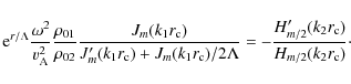 |
(31) |
The dispersion relation (31) is a transcendental equation for the complex frequency
| |
Figure 3:
Real
|
| Open with DEXTER | |
The numerical solution of Eq. (31) shows that the dispersion
equation has a real solution with a cut-off frequency
![]() ,
and complex solutions with very small
imaginary parts. Figure 3 shows the dependence of the real (left
panel) and the imaginary (right panel) parts of the frequency on the
cavity size
,
and complex solutions with very small
imaginary parts. Figure 3 shows the dependence of the real (left
panel) and the imaginary (right panel) parts of the frequency on the
cavity size ![]() .
The real part of the frequency decreases with
increasing
.
The real part of the frequency decreases with
increasing ![]() ,
as expected. The damping time of the oscillations
,
as expected. The damping time of the oscillations
![]() (
(
![]() )
is very
long, which indicates there is almost no wave leakage in the canopy
region. This means that the first few harmonics are trapped in the
cavity. It must be mentioned that the frequencies of first few
harmonics (left panel of Fig. 3) are almost identical to the
frequencies obtained with the free-boundary condition (Fig. 2).
Thus, the oscillation spectrum does not depend significantly on the
choice of the boundary conditions.
)
is very
long, which indicates there is almost no wave leakage in the canopy
region. This means that the first few harmonics are trapped in the
cavity. It must be mentioned that the frequencies of first few
harmonics (left panel of Fig. 3) are almost identical to the
frequencies obtained with the free-boundary condition (Fig. 2).
Thus, the oscillation spectrum does not depend significantly on the
choice of the boundary conditions.
It is interesting to find out what happens if the cylindrical canopy
is replaced by a horizontal magnetic field (as could be the case in
the quiet Sun regions far from the network cores). We have analyzed
the spectrum of the field free photospheric area under a horizontal
magnetic canopy. In this configuration there are no trapped
high-frequency (
![]() )
oscillations along the
vertical direction. The damping times of the vertically propagating
waves are about
)
oscillations along the
vertical direction. The damping times of the vertically propagating
waves are about
![]() ,
which indicates their leaky
nature. On the other hand, horizontally propagating waves (with
large horizontal wave numbers) have real frequencies. But since
their velocities are almost horizontal they cannot be seen in
Doppler velocity power maps. Any initial pulse or wave train will
quickly be dispersed in the horizontal direction. Therefore, these
modes cannot form the observed high-frequency halos.
,
which indicates their leaky
nature. On the other hand, horizontally propagating waves (with
large horizontal wave numbers) have real frequencies. But since
their velocities are almost horizontal they cannot be seen in
Doppler velocity power maps. Any initial pulse or wave train will
quickly be dispersed in the horizontal direction. Therefore, these
modes cannot form the observed high-frequency halos.
4 Excitation by a pressure pulse
The solar photosphere is very dynamic and contains many different
types of impulsive sources. For example, the eruption of new
granules, magnetic-field reconnection events just under the solar
surface, and various other explosive events may take place there.
Therefore, the excitation of pressure and velocity pulses seems to
be quiet common under photospheric conditions. In this section, we
study the propagation of such a pressure pulse (which corresponds to
a density pulse in the isothermal approximation) in the cavity
region. For simplicity, we assume that the pulse has a
![]() -function shape in space and time.
-function shape in space and time.
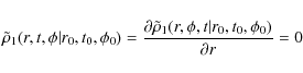
Mathematically this corresponds either to the solution of Eq. (19)
with impulsive initial and boundary conditions or to the solution of
that equation with an additional term modeling the impulsive
external forcing. The equation can then be written as (with the
driving force term in the righthand side)
 |
+ | ![$\displaystyle {1\over r^2}
\frac{\partial ^{2}\tilde{\rho }_{1}}{\partial \phi^...
... ^{2}\tilde{\rho }_{1}}{\partial
t^{2}}+\omega^2_{\rm ac}\tilde{\rho_1}\right]=$](/articles/aa/full_html/2009/38/aa11484-08/img87.png) |
|
| - | (32) |
where r0,
If we consider the case when
 |
(33) |
for t<t0, then
![$\displaystyle \tilde\rho_1(r,t,\phi\vert r_0,t_0,\phi_0)={A_0\delta(t-t_0-R/c_0...
...^2-{(R/c_{0})^2}}\right]\over
c_0 \sqrt{(t-t_0)^2-(R/c_{0})^2}} H(t-t_0-R/c_0),$](/articles/aa/full_html/2009/38/aa11484-08/img93.png) |
(34) |
where A0 is a constant,

and H denotes the Heaviside step function.
| |
Figure 4: Source point, observation point at t>t0, and canopy/cavity interface. |
| Open with DEXTER | |
The first term on the right hand side in Eq. (34) describes the
propagation of the pulse. It is followed by a wake which is given by
the second term in Eq. (34). This is a demonstration of a well-known
result (Rae & Roberts 1982; Fleck & Schmitz 1991; Kalkofen et al.
1993; Sutmann et al. 1998; Roberts 2004; Zaqarashvili & Skhirtladze 2008), viz. the presence of a wavefront that moves away from the
point (
![]() )
with speed c0. The disturbance ahead of the
wavefront is at rest, but behind the wavefront, the medium begins to
oscillate at the cut-off frequency
)
with speed c0. The disturbance ahead of the
wavefront is at rest, but behind the wavefront, the medium begins to
oscillate at the cut-off frequency
![]() .
.
Using Eqs. (15), (18), and (34), the density perturbation for
the wake oscillations takes the form (here t0=0 is chosen
without loss of generality):
![\begin{displaymath}\rho _{1}= -{A_0\omega_{\rm ac}{\rm e}^{-r\sin \varphi /2\Lam...
...eft[\omega_{\rm ac}\sqrt{t^2-{(R/
c_{0}})^2}\right]H(t-R/c_0).
\end{displaymath}](/articles/aa/full_html/2009/38/aa11484-08/img97.png) |
(35) |
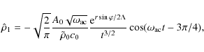
An asymptotic form of the density perturbation can be obtained using the expression of the Bessel function J1 that holds for large arguments
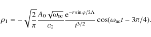 |
(36) |
After the passage of the pressure pulse, the medium density thus oscillates at the cut-off frequency and this oscillation decays asymptotically as 1/t3/2. In fact, the pressure pulse will excite the wide spectrum of oscillations, but the higher frequencies harmonics escape upwards and the lower frequency harmonics are evanescent, so that only the oscillations at the cut-off frequency remain.
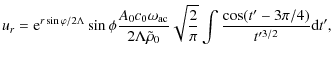
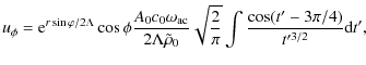
It is interesting to study what happens with the velocity
perturbations in this asymptotic case (
![]() ). Combining
Eqs. (10), (11), and (34), we obtain
). Combining
Eqs. (10), (11), and (34), we obtain
 |
(37) |
and
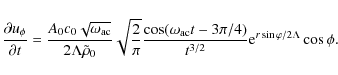 |
(38) |
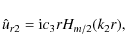
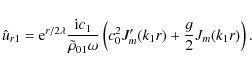
The integration of Eqs. (37) and (38) with respect to time and using the conditions ur=0 and
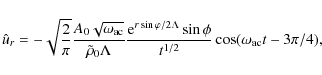 |
(39) |
and
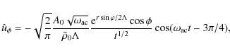 |
(40) |
where
![\begin{figure}
\par\includegraphics[width=9cm,clip]{11484fg5}
\end{figure}](/articles/aa/full_html/2009/38/aa11484-08/img111.png) |
Figure 5:
The density fluctuation after the propagation of pulse as a
function of time and radial coordinate at
|
| Open with DEXTER | |
Figure 5 shows a plot of the density fluctuation, given by Eq. (35)
(the time is normalized to the cut-off frequency,
![]() ,
and the radial coordinate is normalized by the scale height,
,
and the radial coordinate is normalized by the scale height,
![]() ). It is seen that the propagation of the pulse is
followed by a weak amplitude wake that oscillates with the cut-off
period. The amplitude of both the pulse and the wake decrease with
height/time. However, it must be mentioned that the normalized
perturbation of the density,
). It is seen that the propagation of the pulse is
followed by a weak amplitude wake that oscillates with the cut-off
period. The amplitude of both the pulse and the wake decrease with
height/time. However, it must be mentioned that the normalized
perturbation of the density,
![]() ,
increases with r.
The normalized amplitude of the density perturbation in the
asymptotic form, can be written as
,
increases with r.
The normalized amplitude of the density perturbation in the
asymptotic form, can be written as
 |
(41) |
where

The normalized amplitude of the asymptotic density perturbation depends on the direction of propagation (i.e. on the
Figure 7 shows the dependence of the asymptotic velocity wake on the
azimuthal angle, ![]() .
It is clear that the radial component has a
maximum amplitude in the vertical direction, while the azimuthal
velocity component has a maximal amplitude close to
.
It is clear that the radial component has a
maximum amplitude in the vertical direction, while the azimuthal
velocity component has a maximal amplitude close to
![]() .
.
![\begin{figure}
\par\includegraphics[width=9cm,clip]{11484fg6}
\end{figure}](/articles/aa/full_html/2009/38/aa11484-08/img119.png) |
Figure 6:
Normalized asymptotic amplitude of the density wake versus
the azimuthal angle |
| Open with DEXTER | |
5 The energy propagation
Our calculations show clearly that at t=0 the energy is
concentrated in the initial pressure pulse and that it propagates
away as time elapses. The initial pulse, which travels at the sound
speed, carries most of the energy injected into the medium. We can
write down an expression for the asymptotic total energy density for
the wake oscillation, which is the sum of the kinetic and acoustic
potential energy densities
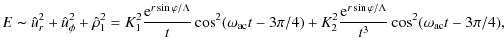 |
(42) |
where

and

It is clear from Eq. (42) that the potential part of the wake energy decays much faster than the kinetic part. Therefore, after some time only the velocity oscillations remain, while the density oscillations have decayed. Furthermore, the total energy is greatest in the vertical direction (at
6 Discussion and conclusions
We have carried out a linear perturbation analysis of the
two-dimensional wave propagation in a stratified, field-free cavity,
which is located under a chromospheric cylindrical magnetic canopy.
We considered the higher density in the cavity than in the overlying
magnetic canopy region (due to the sharp density gradient between
the photosphere and the chromosphere). Then the free boundary
condition at canopy/cavity interface leads to the spectrum of
acoustic oscillation in the cavity. We also examined the response of
the cavity to the propagation of a pressure pulse, which can be
excited in the lower regions by various sources, including
small-scale magnetic reconnection events. It has been shown that the
cavity, which has a radius comparable to the granular dimensions
(![]() 500 km), supports trapped oscillations with periods of
1.5-2 min (cf. Figs. 2, 3). However, one of the oscillation
modes in the cavity is the oscillation with the cut-off frequency.
Furthermore, the frequency of the acoustic modes also has the
tendency to approach the cut-off value for large-scale granular size
(cf. Fig. 2). On the other hand, it has been shown that a pressure
pulse propagating through the cavity sets up a wake, oscillating at
the cut-off frequency. The wake oscillation will resonate with a
free oscillating mode of the cavity, which may lead to an enhanced
acoustic power at the same frequency.
500 km), supports trapped oscillations with periods of
1.5-2 min (cf. Figs. 2, 3). However, one of the oscillation
modes in the cavity is the oscillation with the cut-off frequency.
Furthermore, the frequency of the acoustic modes also has the
tendency to approach the cut-off value for large-scale granular size
(cf. Fig. 2). On the other hand, it has been shown that a pressure
pulse propagating through the cavity sets up a wake, oscillating at
the cut-off frequency. The wake oscillation will resonate with a
free oscillating mode of the cavity, which may lead to an enhanced
acoustic power at the same frequency.
There have been several different explanations of power halos in the literature: (i) the enhancement of acoustic emission by some unknown source (Braun et al. 1992; Brown et al. 1992; Jain & Haber 2002); (ii) incompressible oscillations, such as Alfvén waves or transverse kink waves, in magnetic tubes (Hindman & Brown 1998); (iii) the interaction of acoustic waves with the overlying magnetic canopy (Muglach et al. 2005; Kuridze et al. 2008); and (iv) a change of the spatial-temporal spectrum of the turbulent convection in the magnetic field (Jacoutot et al. 2008). However, observations show a lack of power halos in the intensity maps (Hindman & Brown 1998; Jain & Haber 2002; Muglach et al. 2005; Nagashima et al. 2007), which needs an adequate explanation. These observations challenge the model of the power halos as the result of acoustic waves. However, our model easily explains the discrepancy.
![\begin{figure}
\par\includegraphics[width=9cm,clip]{11484fg7}\par\includegraphics[width=9cm,clip]{11484fg8}
\end{figure}](/articles/aa/full_html/2009/38/aa11484-08/img125.png) |
Figure 7:
Normalized asymptotic amplitudes of the velocity
perturbation components versus |
| Open with DEXTER | |
![\begin{figure}
\par\includegraphics[width=9cm,clip]{11484fg9}
\end{figure}](/articles/aa/full_html/2009/38/aa11484-08/img126.png) |
Figure 8:
Normalized total energy density with respect to |
| Open with DEXTER | |
We suggest that the surroundings of the magnetic network cores and the active regions consist of many small-scale, closed, magnetic-canopy structures (McIntosh & Judge 2001; Schrijver & Title 2003). Granular motions transport the magnetic field at the boundaries and consequently create field-free cylindrical cavity areas under the canopy (Fig. 1). The pressure pulses excited in a lower region propagate through the cavity and leave behind wakes oscillating at the cut-off frequency. These wake oscillations resonate with the free oscillation modes of the cavity. Therefore, the cavities accumulate acoustic oscillations with the observed frequency. However, the amplitude of the density perturbation in the wakes decreases in time faster (viz. as t-3/2) than the amplitude of velocity perturbations (viz. as t-1). Therefore, the density perturbations quickly decay leaving only the velocity oscillations. This explains why the power halos are only seen in the velocity power maps.
Thus, our model suggests that the high-frequency acoustic
oscillations should be trapped around the magnetic network cores and
the active regions, where acoustic cavities can be formed under
small-scale cylindrical magnetic canopies. The deduced oscillation
periods are within 1.5-2 min for cavities with granular sizes,
but the cavities should also oscillate with the photospheric cut-off
frequency. However, the picture will be different far away from the
network cores and active regions, where the cylindrical bipolar
magnetic fields are probably replaced by almost a horizontal
magnetic canopy that has been used as a model for a long time (Evans
& Roberts 1990). In this case, the higher frequency oscillations
propagate upwards (only trapped cut-off modes appear) and,
consequently, power halos cannot be formed. The oscillation at
cut-off frequency should have a small amplitude there, as the
rectangular vertical cavity does not have any oscillation mode with
this frequency. The wake oscillating at cut-off frequency should be
observed there, but with a smaller amplitude, as almost the whole
initial energy is carried away by an initial pulse or a wave train.
Therefore, it is the cylindrical structure of the field-free regions
(see Fig. 1), that helps to trap acoustic waves as the oscillations
occur partly along the ![]() -direction. This explains why the
``power halos'' and ``magnetic shadows'' are observed only near the
quiet-Sun chromospheric magnetic network cores (McIntosh & Judge
2001; Krijger et al. 2001; Vecchio et al. 2007).
-direction. This explains why the
``power halos'' and ``magnetic shadows'' are observed only near the
quiet-Sun chromospheric magnetic network cores (McIntosh & Judge
2001; Krijger et al. 2001; Vecchio et al. 2007).
It must be noted that intensity halos are visible in the magnetic canopy regions in some observations (Moretti et al. 2007). However, this is consistent with our model. As mentioned before, our calculation does not include the exact solution in the overlying magnetic canopy region because of mathematical difficulties. On the other hand, the free oscillations of the cavity/canopy interface may excite oscillations in the overlying region as observed by Moretti et al. (2007). Likewise, the oscillations of the cavity may excite transverse waves in an overlying magnetic canopy, which can be checked by observations of the magnetic field oscillation in the power-halo regions.
Acknowledgements
This work was supported by Georgian National Science Foundation grant GNSF/ST06/4-098. D.K. is grateful for kind hospitality at the Center for Plasma Astrophysics, K.U. Leuven, during his visit when the significant parts of the work were developed. These results were obtained in the framework of the projects GOA/2009-009 (K.U. Leuven), G.0304.07 (FWO-Vlaanderen), and C 90347 (ESA Prodex 9). T.Z. acknowledges Austrian Fond zur Förderung der wissenschaftlichen Forschung (project P21197-N16).
Appendix A: Derivation of the velocity components
Integration of Eqs. (37) and (38) gives
 |
(A.1) | ||
 |
(A.2) |
where
Integral in Eqs. (A.1), (A.2) can be solved as
| I | = |  |
|
| = |  |
||
| = | ![$\displaystyle \cos{3\pi\over 4}\left[ -{2\cos t'\over t'^{1/2}}-2\sqrt{2\pi}
S\left(\sqrt{2t'/\pi}\right)+F_1\right]$](/articles/aa/full_html/2009/38/aa11484-08/img132.png) |
||
![$\displaystyle +\sin{3\pi\over 4}\left[ -{2\sin t'\over t'^{1/2}}+2\sqrt{2\pi}
C\left(\sqrt{2t'/\pi}\right)+F_2\right]$](/articles/aa/full_html/2009/38/aa11484-08/img133.png) |
|||
| = | ![$\displaystyle -{2\over t'^{1/2}}\left[\cos{3\pi\over 4}\cos t'+\sin{3\pi\over
4}\sin t' \right]$](/articles/aa/full_html/2009/38/aa11484-08/img134.png) |
||
![$\displaystyle +2\sqrt{\pi}\left[S\left(\sqrt{2t'/\pi}\right)+C\left(\sqrt{2t'/\pi}\right)\right]+{\sqrt{2}\over
2}\left(F_2-F_1\right)$](/articles/aa/full_html/2009/38/aa11484-08/img135.png) |
|||
| = | |||
 |
(A.3) |
where F1, F2 are the integration constants, and S and Care the Fresnel sine and cosine integral functions, respectively. Fresnel functions tend to 1/2 for large arguments, therefore we have
 |
(A.4) |
where
![]() should tend to zero when
should tend to zero when
![]() ;
therefore,
;
therefore,
 |
(A.5) |
which gives
 |
(A.6) |
Substitution of the expression (A.6) into Eqs. (A.1), (A.2) gives Eqs. (39) and (40).
References
- Abramowitz, M., & Stegun, I. A. 1967, Handbook of Mathematical Functions (New York: Dover Publications) (In the text)
- Bodo, G., Kalkofen, W., Massaglia, S., & Rossi, P. 2000, A&A, 354, 296 [NASA ADS]
- Braun, D. C., Lindsey, C., Fan, Y., & Jefferies, S. M. 1992, ApJ, 392, 739 [NASA ADS] [CrossRef] (In the text)
- Brown, T. M., Bogdan, T. J., Lites, B. W., & Thomas, J. H. 1992, ApJ, 394, 65 [NASA ADS] [CrossRef] (In the text)
- Centeno, R., Socas-Navarro, H., Lites, B., et al. 2007, ApJ, 666, 137 [NASA ADS] [CrossRef]
- de Wijn, A. G., Rutten, R. J., Haverkamp, E. M. W. P., & Sutterlin, P. 2005, A&A, 441, 1183 [NASA ADS] [CrossRef] [EDP Sciences]
- Erdélyi, R., Malins, C., Toth, G., & de Pontieu, B. 2007, A&A, 461, 1299 [NASA ADS] [CrossRef] (In the text)
- Evans, D. J., & Roberts, B. 1990, ApJ, 356, 704 [NASA ADS] [CrossRef] (In the text)
- Fontenla, J. M., Avrett, E. H., & Loeser, R. 1990, ApJ, 355, 700 [NASA ADS] [CrossRef] (In the text)
- Fleck B., & Schmitz, F. 1991, A&A, 250, 235 [NASA ADS] (In the text)
- Jacoutot, L., Kosovichev, A. G., Wray, A., & Mansour, N. N. 2008, ApJ, 684, 51 [NASA ADS] [CrossRef] (In the text)
- Jain, R., & Haber, D. 2002, A&A, 387, 1092 [NASA ADS] [CrossRef] [EDP Sciences] (In the text)
- Hindman, B. W., & Brown, T.M. 1998, ApJ, 504, 1029 [NASA ADS] [CrossRef] (In the text)
- Hanasoge, S. M. 2008, ApJ, 680, 1457 [NASA ADS] [CrossRef] (In the text)
- Kahn, P.B. 1990, Mathematical Methods for Scientists and Engineers (John Wiley & Sons), 208 (In the text)
- Kalkofen, W., Rossi, P., Bodo, G., & Massaglia, S. 1994, A&A, 279, 579
- Krijger, J. M., Rutten, R. J., Lites, B. W., et al. 2001, A&A, 379, 1052 [NASA ADS] [CrossRef] [EDP Sciences] (In the text)
- Kuridze, D., Zaqarashvili, T. V., Shergelashvili, B. M., & Poedts, S. 2008, Annales Geophysicae, 26, 10, 2983 (In the text)
- Lamb, H. 1908, Proc. Lond. Math. Soc., Ser., 2, 7, 122 (In the text)
- McIntosh, S. W., & Judge, P.G. 2001, ApJ, 561, 420 [NASA ADS] [CrossRef] (In the text)
- Moretti, P. F., Jefferies, S. M., Armstrong, J. D., & Mc Intosh, S. W. 2007, A&A, 471, 961 [NASA ADS] [CrossRef] [EDP Sciences] (In the text)
- Morse P. M., & Feshbach H. 1953, Methods of Theoret. Physics Part I (New York: Mc Graw Hill) (In the text)
- Muglach, K., Hofmann, A., & Staude, J. 2005, A&A, 437, 1055 [NASA ADS] [CrossRef] [EDP Sciences] (In the text)
- Nagashima, K., Sekii, T., Kosovichev, A. G., et al. 2007, PASJ, 59, 631 [NASA ADS] (In the text)
- Rae I. C., & Roberts, B. 1982, ApJ, 256, 761 [NASA ADS] [CrossRef] (In the text)
- Roberts, B. 2004, ESA SP-547, 1 (In the text)
- Schrijver, C. J., & Title, A. M. 2003, ApJ, 597, L165 [NASA ADS] [CrossRef] (In the text)
- Srivastava, A. K., Kuridze, D., Zaqarashvili, T. V., & Dwivedi B. N. 2008, A&A, 481, 95 [NASA ADS] [CrossRef] (In the text)
- Sutmann, G., Musielak, Z. E., & Ulmschneider, P. 1998, A&A, 340, 556 [NASA ADS] (In the text)
- Vecchio, A., Cauzzi, G., Reardon, K. P., Janssen, K., & Rimmele, T. 2007, A&A, 461, 1 [NASA ADS] [CrossRef] [EDP Sciences] (In the text)
- Vernazza, J. E., Avrett, E. H., & Loeser, R. 1981, ApJS, 45, 635 [NASA ADS] [CrossRef] (In the text)
- Zaqarashvili, T. V., & Skhirtladze, N. 2008, ApJ, 683, 91 [NASA ADS] [CrossRef] (In the text)
All Figures
| |
Figure 1: Simple schematic picture of small-scale magnetic canopy overlying a field-free cavity with gravitational stratification, g. |
| Open with DEXTER | |
| In the text | |
| |
Figure 2:
The oscillation frequency, |
| Open with DEXTER | |
| In the text | |
| |
Figure 3:
Real
|
| Open with DEXTER | |
| In the text | |
| |
Figure 4: Source point, observation point at t>t0, and canopy/cavity interface. |
| Open with DEXTER | |
| In the text | |
| |
Figure 5:
The density fluctuation after the propagation of pulse as a
function of time and radial coordinate at
|
| Open with DEXTER | |
| In the text | |
| |
Figure 6:
Normalized asymptotic amplitude of the density wake versus
the azimuthal angle |
| Open with DEXTER | |
| In the text | |
| |
Figure 7:
Normalized asymptotic amplitudes of the velocity
perturbation components versus |
| Open with DEXTER | |
| In the text | |
| |
Figure 8:
Normalized total energy density with respect to |
| Open with DEXTER | |
| In the text | |
Copyright ESO 2009
Current usage metrics show cumulative count of Article Views (full-text article views including HTML views, PDF and ePub downloads, according to the available data) and Abstracts Views on Vision4Press platform.
Data correspond to usage on the plateform after 2015. The current usage metrics is available 48-96 hours after online publication and is updated daily on week days.
Initial download of the metrics may take a while.