| Issue |
A&A
Volume 505, Number 2, October II 2009
|
|
|---|---|---|
| Page(s) | 801 - 810 | |
| Section | The Sun | |
| DOI | https://doi.org/10.1051/0004-6361/200810946 | |
| Published online | 03 August 2009 | |
Properties of magnetic elements in the quiet Sun using the marker-controlled watershed method
Z. X. Xie1 - D. R. Yu1 - J. Zhang2 - S. H. Yang2 - Q. H. Hu1
1 - Harbin Institute of Technology, Harbin 150001, PR China
2 -
National Astronomical Observatories, Chinese Academy of Sciences, Beijing 100012, PR China
Received 10 September 2008 / Accepted 19 June 2009
Abstract
Context. The quiet Sun is an important part of understanding the global magnetic properties of the Sun. A recently launched observation system, named HINODE, provides a lot of high-resolution images for studying the quiet Sun. Obviously, it is time-consuming to analyze these images by hand. It is desirable to develop a technique for recognizing magnetic elements, thus automatically computing magnetic properties and the relationship between magnetic elements and granulation.
Aims. We design an automatic method of recognizing magnetic elements based on the features of HINODE magnetograms and of measuring their properties. Then we study the relationship between magnetic elements and granulation.
Methods. We used the magnetogram, continuum image, and Dopplergram on April 16, 2007, which were taken with the Solar Optical Telescope instrument aboard HINODE. The field of view is 147
![]()
![]()
![]() 30 in a quiet solar region, locating at disk center. We introduced the mark-controlled watershed method to detect magnetic elements automatically, because it is a popular image-segmentation method for dealing with overlapping objects. We took the centers that are the local maximum in all directions as the marks for restraining over-segmentation. We computed the properties of the detected magnetic elements and the relation among magnetic field strength, relative continuum intensity, and Doppler velocity at the same locations of magnetic elements.
30 in a quiet solar region, locating at disk center. We introduced the mark-controlled watershed method to detect magnetic elements automatically, because it is a popular image-segmentation method for dealing with overlapping objects. We took the centers that are the local maximum in all directions as the marks for restraining over-segmentation. We computed the properties of the detected magnetic elements and the relation among magnetic field strength, relative continuum intensity, and Doppler velocity at the same locations of magnetic elements.
Results. We obtain the following results: (1) 34% of our observation region are covered by magnetic fields; (2) the magnetic flux distribution of all elements reaches a peak at
![]() Mx for the whole region; (3) the relative continuum intensity distribution at the locations of magnetic elements reaches a peak at 0.97, which shows that the majority of magnetic elements located at the areas where the relative continuum intensity is less than its average. The relative continuum intensities in the areas with strong flux density are the median, meaning that the strong magnetic elements are usually located at the boundary of granulation; (4) the absolute Doppler velocity distribution at the locations of magnetic elements reaches a peak at 1.00 km s-1, and the majority of weak magnetic elements located at the areas where the absolute velocity is greater than 1.00 km s-1; (5) strongly magnetized regions only have weak absolute Doppler velocities. The absolute velocity is lower than 1.00 km s-1 in the regions where the magnetic flux density of elements is higher than 100 G.
Mx for the whole region; (3) the relative continuum intensity distribution at the locations of magnetic elements reaches a peak at 0.97, which shows that the majority of magnetic elements located at the areas where the relative continuum intensity is less than its average. The relative continuum intensities in the areas with strong flux density are the median, meaning that the strong magnetic elements are usually located at the boundary of granulation; (4) the absolute Doppler velocity distribution at the locations of magnetic elements reaches a peak at 1.00 km s-1, and the majority of weak magnetic elements located at the areas where the absolute velocity is greater than 1.00 km s-1; (5) strongly magnetized regions only have weak absolute Doppler velocities. The absolute velocity is lower than 1.00 km s-1 in the regions where the magnetic flux density of elements is higher than 100 G.
Key words: Sun: magnetic fields - Sun: granulation - methods: observational
1 Introduction
The quiet region of the solar photosphere covers more than 90% of the solar surface and provides a large fraction of magnetic flux and energy even in solar maximum years (Harvey-Angle 1993). It is important to understand the global magnetic properties of the Sun, such as the structure of the quiet corona (Schrijver & Title 2003), the chromospheric heating (Rezaei et al. 2007a), the sources of the solar wind, and the emergence of magnetic flux. The magnetic field in the quiet region consists of three types: ephemeral regions (Harvey & Martin 1973), network fields (Leighton et al. 1962), and intranetwork (IN) fields (Smithson 1975; Livingston & Harvey 1975).
Our knowledge of the quiet Sun's magnetic fields has improved
dramatically with observations and numerical simulations. The nature
of its magnetic fields have been studied
(Schrijver et al. 1997; Hagenaar 2001; Hagenaar et al. 1999) with data
from SOHO/MDI (Scherrer et al. 1995). Using time sequences of deep
magnetograms obtained at the Big Bear Solar Observatory (BBSO), The
morphology dynamics of network and IN were analyzed, such as mean
horizontal velocity fields of IN and network fields, by using the
local correlation tracking technique
(Wang et al. 1996), the lifetime of IN elements (Zhang et al. 1998b),
and motion patterns and evolution of IN and network magnetic fields
(Zhang et al. 1998d,c; Liu et al. 1994). The strength and
distribution of magnetic fields for network and/or IN elements have
been discussed by many researchers. Keller et al. (1994) provide
an excellent summary of observations of IN magnetism to that date.
Lin (1995) studied the distribution of magnetic field in both the
active and quiet Sun using the two magnetically sensitive infrared
Fe I lines at 15 648 Å and 15 652 Å. Wang et al. (1995) analyzed distributions of magnetic elements
on log-log plots using observations made by BBSO. They found that
the distributions of network and IN fluxes show peaks at about
![]() Mx and
Mx and
![]() Mx, respectively.
Schrijver et al. (1997) considered the distribution of fluxes from
a very quiet region of the Sun and found that a single exponential
seemed a reasonable fit to the distribution of fluxes over a narrow
range of fluxes. Parnell (2002) point out that the fluxes
are distributed in the Weibull distribution, which involves a power
law and an exponential.
Mx, respectively.
Schrijver et al. (1997) considered the distribution of fluxes from
a very quiet region of the Sun and found that a single exponential
seemed a reasonable fit to the distribution of fluxes over a narrow
range of fluxes. Parnell (2002) point out that the fluxes
are distributed in the Weibull distribution, which involves a power
law and an exponential.
Parnell et al. (2008) compare the fluxes from MDI with those from
SOT/Hinode. The smallest features in SOT/Hinode have just
![]() 1016 Mx, a factor of thirty less than the smallest
observed by MDI. Through using a ``clumping'' algorithm, the fluxes in
MDI and SOT follow the same distribution - a power law - between
1016 Mx, a factor of thirty less than the smallest
observed by MDI. Through using a ``clumping'' algorithm, the fluxes in
MDI and SOT follow the same distribution - a power law - between
![]() Mx and 1020 Mx. Thus, the mechanism
producing network and intranetwork features appears to be the same.
Furthermore, the power-law index of this distribution is found to be
-1.85. In recent years, many studies have focused on the strength
and flux distribution of IN (Lites et al. 2008; Rezaei et al. 2007b; Sánchez Almeida 2003; Domínguez Cerdeña et al. 2006; Suarez et al. 2007; Socas-Navarro et al. 2004; Domínguez Cerdeña et al. 2003; Lites & Socas-Navarro 2004; Harvey et al. 2007; Sánchez Almeida 2007).
Mx and 1020 Mx. Thus, the mechanism
producing network and intranetwork features appears to be the same.
Furthermore, the power-law index of this distribution is found to be
-1.85. In recent years, many studies have focused on the strength
and flux distribution of IN (Lites et al. 2008; Rezaei et al. 2007b; Sánchez Almeida 2003; Domínguez Cerdeña et al. 2006; Suarez et al. 2007; Socas-Navarro et al. 2004; Domínguez Cerdeña et al. 2003; Lites & Socas-Navarro 2004; Harvey et al. 2007; Sánchez Almeida 2007).
The relation between quiet Sun magnetic fields and convection also have been discussed. Title et al. (1987) point out that magnetic fields in the network correlate better with dark intergranular lanes than with bright granules. A lot of high spatial resolution observations showed that small-scale magnetic features are related to the photospheric filigree bright points (Keller 1992; Title et al. 1992). By analyzing fine photospheric filtergrams and their corresponding magnetic features, Zhang et al. (1998a) concluded that the relationship between the fine bright structures in the photospheric filtergrams and the longitudinal magnetic field is complex. Although most bright points correspond to small-scale magnetic features in the magnetograms, some photospheric bright features also occur in the spaces between magnetic features. Lin & Rimmele (1999) use new data at 1'' pixel resolution to demonstrate that there are weak magnetic fields with mixed polarities closely associated with the solar granulation both in spatial distribution and time evolution. Compared with simultaneous high-resolution granulation images, these data also reveal many interesting MHD processes never observed before, such as the creation of kilogauss magnetic features associated with the development of intergranular lanes. Using a high spatial resolution observation in the magnetically sensitive Fe I 630.25 nm line, Stolpe & Kneer (2000) find that the weak flux may appear almost everywhere in the granular pattern, with a 65% preference for intergranular spaces.
To study the properties of the Sun, a number of observation instruments have been developed and launched. Missions such as SOHO (Scherrer et al. 1995), TRACE (Handy et al. 1999), GONG (Leibacher 1999, ground-based observatories), and HINODE (Suematsu et al. 2008) are producing far more data than can be analyzed directly by humans. Detection and recognition techniques for analyzing magnetic elements have become an important tool in studying the quiet region. Magnetograms are valuable for detecting magnetic elements automatically.
A review of existing recognition algorithms has been presented by DeForest et al. (2007). Roughly speaking, there are four automatic magnetic-feature recognition codes named CURV (Hagenaar et al. 1999), MCAT (Parnell 2002), SWAMIS (Lamb & Deforest 2003), and YAFTA (Welsch & Longcope 2003). YAFTA uses a simple threshold to detect active regions, because it is far above the noise level. SWAMIS and MCAT use two thresholds: an upper threshold for isolated pixels and a lower one for pixels that are adjacent to already-selected pixels, while CURV uses the curvature and their second derivative to detect the center and the boundary of the magnetic element, respectively. After detecting the pixels of magnetic elements, SWAMIS uses two different methods, downhill and clumping, to identify magnetic elements. Downhill identifies one magnetic element per local maximum region, while clumping identifies all connected pixels into a single magnetic element. Because different magnetic elements have different absolute magnetic flux densities at the center and the boundary, one or two thresholds to segment magnetic elements will lead to including background into strong magnetic elements or taking boundary of weak magnetic elements as background. Moreover, it is difficult for threshold methods to determine the boundary for two adjacent magnetic elements when there is noise in the boundary.
The absolute magnetic flux density at the boundary is zero or above the noise level for isolated magnetic elements; however, the absolute magnetic flux densities at the boundary are different for the adjacent magnetic elements. The key problem to detect magnetic elements is thus to partition the adjacent magnetic elements. Theoretically speaking, the absolute magnetic density from the center toward the boundary of a magnetic element decreases monotonously, and SWAMIS considers that the adjacent magnetic elements meet in a local minimum region. Because of the spatial and temporal noises, the absolute magnetic density may fluctuate from the center to boundary, so if we find some local minimum region, we should identify whether it is a real boundary of the adjacent elements or is just caused by noise. It is obvious that noise does not have a strong influence on centers of magnetic elements. These are the local maximum of absolute magnetic field strengths with respect to its nearest neighbors in all directions. We can therefore use the centers to mark a magnetic element and determine whether a local minimum region is a boundary or noise.
Here, we introduce the mark-controlled watershed method to identify magnetic elements automatically. This method is generalized from watersheds, which is a popular segmentation method for separating touching or adjacent objects (Courses & Surveys 1999; Beucher & Meyer 1993; Tremeau & Colantoni 2000; Haris et al. 1998). However, it has been reported that the watershed algorithm often leads to over-segmentation (Vincent 1993), meaning that the method may partition one magnetic element to a set of small magnetic elements. This may lead to error in the statistics. As we can detect the center of a magnetic element effectively, we use the center as a marker to avoid over-segmentation. Eight neighbors of a marker should have the same polarity and be smaller than or equal to the absolute value of the marker. Furthermore, if the distance between two markers is less than 3 pixels, the pixel with a greater magnetic flux density is marked, while the other is not marked. When using mark-controlled watershed, the pixels around the marker are combined as a magnetic element, and other local maxima/minima are not considered. As we know, all the local maxima/minima are used as seeds to cluster magnetic elements in the traditional watershed, which leads to over-segmentation. However, there is a one-pixel wide boundary line not included in the magnetic element when the watershed technique or the marker-controlled watershed method is used. In this work, we add the boundary pixels to each magnetic element. If several magnetic elements meet at the same boundary pixels, the pixels are randomly allocated to one of these elements. Based on the above idea, we combined the prior information of magnetograms to mark the center of each magnetic element first and used these marks to avoid over-segmentation.
In this paper, we propose a magnetic element detection method
according to the features of magnetogram obtained by the
spectropolarimeter aboard HINODE with a spatial sampling of
0
![]() 16, and compute the flux, area, magnetic field strength, and
fractal dimension of every magnetic element. Then the relation among
magnetic elements, the continuum image, and the Dopplergram is
discussed. The observations and the features of magnetogram are
described in Sect. 2. Section 3
introduces how to find the magnetic elements automatically and
compares our method with SWAMIS-downhill and SWAMIS-clumping
methods. We present the results in Sect. 4, and
Sect. 5 concludes the paper.
16, and compute the flux, area, magnetic field strength, and
fractal dimension of every magnetic element. Then the relation among
magnetic elements, the continuum image, and the Dopplergram is
discussed. The observations and the features of magnetogram are
described in Sect. 2. Section 3
introduces how to find the magnetic elements automatically and
compares our method with SWAMIS-downhill and SWAMIS-clumping
methods. We present the results in Sect. 4, and
Sect. 5 concludes the paper.
2 Observations and feature analysis
| |
Figure 1:
Longitudinal magnetogram ( left), continuum image
( middle), and Dopplergram ( right) of a quiet Sun region obtained at
HINODE on April 16, 2007. The field of view is
147
|
| Open with DEXTER | |
The data sets analyzed here consist of a longitudinal magnetogram, a
continuum image, and a Dopplergram. They were taken on April 16,
2007, with the Solar Optical Telescope
(SOT; Ichimoto et al. 2008; Suematsu et al. 2008; Tsuneta et al. 2008; Shimizu et al. 2008)
instrument aboard HINODE (Kosugi et al. 2007). The
spectro-polarimeter (SP, Lites et al. 2001) in
HINODE/SOT provides observations in four modes (normal,
fast, dynamics, and deep maps) and the SP map adopted here was
observed in normal map mode from 00:23 UT to 01:48 UT, with the
signal-to-noise ratio about 103. The continuum wavelength is
630.08-630.32 nm. Figure 1 shows the magnetogram, the
continuum image, and the Dopplergram. The field of view is
147
![]()
![]()
![]() 30 in a quiet solar region,
located at the disk center. The map is constructed from
30 in a quiet solar region,
located at the disk center. The map is constructed from
![]() full Stokes profiles of the photospheric
Fe I 630.15 nm and 630.25 nm lines and nearby continuum. For
each raster slit, the integrated exposure time is 4.8 s and the
pixel sampling along the slit is 0
full Stokes profiles of the photospheric
Fe I 630.15 nm and 630.25 nm lines and nearby continuum. For
each raster slit, the integrated exposure time is 4.8 s and the
pixel sampling along the slit is 0
![]() 16. The scan is in the
east-west direction with the scanning step of about 0
16. The scan is in the
east-west direction with the scanning step of about 0
![]() 15.
15.
The Stokes spectrum inversion code based on the assumption of
Milne-Eddington atmospheres (Yokoyama, private communication) is
an effective means of deriving vector magnetic fields, Doppler
shifts, and also continuum intensities from the Stokes profiles. The
vector magnetic field B is shown with the longitudinal field
(1-![]() )B
)B![]() (
(![]() )
and the transverse field
(1-
)
and the transverse field
(1-![]() )1/2B
)1/2B![]() (
(![]() ), where
), where ![]() is
the stray light fraction and
is
the stray light fraction and ![]() the inclination angle
corresponding to line-of-sight direction. Then the Doppler shifts
are derived according to the Fe I 6302.5 Stokes I profiles
and averaged over the whole field-of-view. We only analyzed the
pixels with total polarization degree above one times the noise
level
the inclination angle
corresponding to line-of-sight direction. Then the Doppler shifts
are derived according to the Fe I 6302.5 Stokes I profiles
and averaged over the whole field-of-view. We only analyzed the
pixels with total polarization degree above one times the noise
level
![]() in the polarization continuum.
in the polarization continuum.
As we know, there are three parts in the magnetogram: positive
magnetic elements, negative magnetic elements, and background. The
pixel values of positive and negative magnetic elements are higher
and lower than 0, respectively, while the pixel values of background
are equal to 0, so the background can be easily recognized.
Theoretically speaking, the absolute flux density ![]() of a
magnetic element can be described by a two-dimensional Gaussian
function (Hagenaar et al. 1999):
of a
magnetic element can be described by a two-dimensional Gaussian
function (Hagenaar et al. 1999):
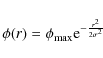 |
(1) |
where
or
where
Table 1: Location information of pixels around the center of a magnetic element.
3 Magnetic element segmentation with the marker-controlled watershed technique
| |
Figure 2: Effectiveness of the marks. The first panel is a small part of the original magnetogram. The second panel is the topographic surface of the first panel region. The third panel shows the watershed results. The fourth panel illustrates the mark-controlled watershed results. |
| Open with DEXTER | |
| |
Figure 3: Segmentation of magnetic elements. Image 1 is center, white rectangle region of magnetogram in Fig. 1. Image 2 is segmentation results. Image 3 marks the center of each magnetic element in the original magnetogram. Image 4 marks the boundary of each magnetic element in the original magnetogram. |
| Open with DEXTER | |
The watershed method is a region-growing algorithm that takes an image as a topographic surface (Meyer & Beucher 1990). It uses a flooding process to search the watershed lines. If we consider the image as a topographic relief, where the height of each point is directly related to its gray level and rain gradually falls on the terrain, the watersheds are the lines that separate the catchment basins. Contacting points between the propagation originating from different minima are defined as the boundaries of the regions and are used to create the final partition.
In practice, the classical watershed method often leads to over-segmentation caused by noise and local irregularities. Two approaches were developed to deal with this problem. The first one involves merging adjacent regions according to some criterion after the use of the watershed algorithm (Courses & Surveys 1999; Tremeau & Colantoni 2000; Haris et al. 1998). The second one uses markers to reduce over-segmentation (Salembier & Marques 1999; Salembier & Pardas 1994). Since we can get the centers of magnetic elements as markers, we chose the second approach. We have two classes of makers: internal markers associated with the objects of interest and external markers associated with the background. A marker is a connecting region belonging to an object indicating the presence of an object. Figure 2 displays the effectiveness of the technique. The first panel is a part of the original magnetogram. The second panel is the topographic surface of the selected region, where the horizontal and vertical dimensions are the locations of pixels and the third dimension gives the pixel value. We can detect three magnetic elements in the first panel using eyes. However, from the topographic surface, we can see more than three local minima, which are black. We used the classical watershed method on the magnetogram, and the detection result is shown in the third panel of Fig. 2. We can find that 8 magnetic elements are detected. However, if we use the centers of magnetic elements based on Eq. (3) to guide segmentation, only 3 local minimum are marked, shown in the fourth panel, where the three isolated bright points are the centers and the adjacent white lines are the boundaries of these three elements.
![\begin{figure}
\par\includegraphics[width=18cm,clip]{10946fig4.eps}
\end{figure}](/articles/aa/full_html/2009/38/aa10946-08/img29.png) |
Figure 4: Results of different magnetic element detection methods. (1) White rectangle region of original magnetogram in Fig. 1. (2) Marker-controlled watershed. (3) Downhill identifies one magnetic element per local maximum region. (4) Clumping identifies all connected above-threshold pixels into a single magnetic element. |
| Open with DEXTER | |
![\begin{figure}
\par\includegraphics[width=18cm,clip]{10946fig5.eps}
\end{figure}](/articles/aa/full_html/2009/38/aa10946-08/img30.png) |
Figure 5: Log-log magnetic flux distribution of positive and negative magnetic elements in the longitudinal magnetogram with three different automatic detection methods. The first panel is with the marker-controlled watershed, the second one with downhill, the third with clumping. |
| Open with DEXTER | |
To process images with matlab, the magnetogram is mapped into interval [0, 255], so the maximal pixel value is 255, the minimal pixel value is 0, while the background is 127. According to the maker-controlled watershed algorithm, we know that the locally minimal value in a image is the center of an object and the locally greatest value is the boundary of objects. We should therefore detect the positive and negative magnetic elements separately. We specify the pixel value of positive magnetic elements as their complement.
To detect the negative magnetic elements, a typical procedure for the marker-controlled watershed method consists of 4 steps. (1) The positive magnetic elements are masked as background. That is to say, the pixel values higher than 127 are set at 127. (2) The center of each negative magnetic element is labeled. The pixels which are satisfied Eq. (3) are labeled. We use these labels to smooth the image generated in step 1. Morphological reconstruction is introduced to smooth the local minima without labels, and only the minima with the marked labels are used as the centers of magnetic elements (Rivest et al. 2005). (3) We compute the watershed lines of the smoothed image with the markers. (4) The common boundary of some adjacent magnetic elements is separated into these fields arbitrarily. After the above 4 steps, we can get the centers and boundaries of all the negative magnetic elements. Then we give each negative magnetic element a unique label.
When detecting positive magnetic elements, the procedures are the same as the described above except the steps 1 and 2. In step 1, the pixel values that are less than 127 are set at 127. Because the center of a positive element is the local maximum, we compute the complement of the gray image. Thus the local maximum becomes a local minimum. Then the watershed algorithm can be used. In step 2, we use Eq. (2) to find the centers of positive fields.
To reduce the influence of noise, we exclude the magnetic elements with less than nine contiguous pixels. The detection result of positive and negative magnetic elements is shown in Fig. 3. The first panel of Fig. 3 is the original image, and the second panel is the segmented image. The third panel marks the center of each magnetic element on the original image, and the fourth panel marks the boundary of each magnetic element on the original image. We can see that almost all the magnetic elements found by hand is detected with this watershed method. Moreover, the boundary of each weak magnetic element is also found. Figure 4 shows the results of different magnetic element detection methods. In our observations, we only analyzed the pixels with total polarization degree above the noise level in the polarization continuum. ``Downhill'' identifies one magnetic element per local maximum region, while ``clumping'' identifies all connected pixels into a single magnetic element. And we also excluded magnetic elements less than nine contiguous pixels.
After identifying the markers according to the above conditions, our method can identify one magnetic element per marker. From the segmentation results, we can arrive at the following conclusions. 1) For isolated magnetic elements, our method get the same results as clumping, while downhill always separates one into several small parts. 2) For adjacent magnetic elements, the clumping identifies all connected pixels, while our method splits the block into several magnetic elements according to the markers, and downhill still separates one magnetic element into many small fragments.
4 Results and analysis
In Sect. 3 we show a technique to detect the positive and negative magnetic elements on the magnetogram. In this section we analyze the physical parameters of magnetic elements, such as the flux, area, magnetic strength, and fractal dimension. Then the relationship of the magnetogram, the continuum image, and the Dopplergram is discussed.
![\begin{figure}
\par\includegraphics[width=18cm,clip]{10946fig6.eps}
\end{figure}](/articles/aa/full_html/2009/38/aa10946-08/img31.png) |
Figure 6: Log-log area distribution of positive and negative magnetic elements in the longitudinal magnetogram using three different automatic detection methods. The first panel is with the marker-controlled watershed, the second with downhill, the third with clumping. |
| Open with DEXTER | |
![\begin{figure}
\par\includegraphics[width=18cm,clip]{10946fig7.eps}
\end{figure}](/articles/aa/full_html/2009/38/aa10946-08/img32.png) |
Figure 7: Log-log magnetic flux density distribution of positive and negative magnetic elements in the longitudinal magnetogram with three different automatic detection methods. The first panel is with the marker-controlled watershed, the second with downhill, the third with clumping. |
| Open with DEXTER | |
Table 2: Statistics of magnetic elements with the three different methods.
4.1 The physic parameters of the longitudinal magnetic fields
By using our method, a total of 10 279 magnetic elements are
identified in the longitudinal magnetogram shown in
Fig. 1. Downhill detects 14 248 magnetic elements, while
clumping detects 4837 elements. The statistics with our method,
downhill and clumping are listed in Table 2. The
total area of the magnetogram from our observation is
![]() cm2, while the total area of magnetic fields
is
cm2, while the total area of magnetic fields
is
![]() cm2. That is to say, only about 34% of
our observations are covered by the magnetic field, while 66%
surface in the magnetogram is nonmagnetic. Downhill detects more
elements than our method, while clumping detects fewer elements than
ours. The total flux and area identified by clumping are the largest
compared with the other two methods, and the mean flux and mean area
of magnetic elements with clumping are also the largest. However,
the mean flux density of magnetic elements using clumping is the
lowest, because the mean area of magnetic elements with clumping is
cm2. That is to say, only about 34% of
our observations are covered by the magnetic field, while 66%
surface in the magnetogram is nonmagnetic. Downhill detects more
elements than our method, while clumping detects fewer elements than
ours. The total flux and area identified by clumping are the largest
compared with the other two methods, and the mean flux and mean area
of magnetic elements with clumping are also the largest. However,
the mean flux density of magnetic elements using clumping is the
lowest, because the mean area of magnetic elements with clumping is
![]() cm2, which is a little more than two times the
mean area of elements with the other two methods. The total flux,
the total area, the mean flux, and the mean area of elements with
our method are greater than with downhill, while those with our
method are smaller than with clumping.
cm2, which is a little more than two times the
mean area of elements with the other two methods. The total flux,
the total area, the mean flux, and the mean area of elements with
our method are greater than with downhill, while those with our
method are smaller than with clumping.
Figure 5 illustrates the distributions of
magnetic flux with these three different methods, where positive and
negative magnetic elements are denoted by triangles and asterisks,
respectively. The bin size for magnetic flux is 1015 Mx. In
the first panel with our method, the absolute flux of all magnetic
elements is between
![]() Mx and
Mx and
![]() Mx. The mean flux is
Mx. The mean flux is
![]() Mx, and the
distributions of magnetic flux reach distinct peaks at
Mx, and the
distributions of magnetic flux reach distinct peaks at
![]() Mx,
Mx,
![]() Mx, and
Mx, and
![]() Mx for positive, negative, and all elements,
respectively. For the whole quiet region of our observations, there
is a peak in the log-log magnetic flux distribution of elements.
Although the numbers of positive and negative elements are
different, their distributions are similar to each other. The second
panel is computed with downhill. The range in absolute flux is
between
Mx for positive, negative, and all elements,
respectively. For the whole quiet region of our observations, there
is a peak in the log-log magnetic flux distribution of elements.
Although the numbers of positive and negative elements are
different, their distributions are similar to each other. The second
panel is computed with downhill. The range in absolute flux is
between
![]() Mx and
Mx and
![]() Mx. The mean
absolute flux is
Mx. The mean
absolute flux is
![]() Mx. The third panel shows the
result computed with the clumping method. The absolute flux is
between
Mx. The third panel shows the
result computed with the clumping method. The absolute flux is
between
![]() Mx and
Mx and
![]() Mx. The mean
absolute flux is
Mx. The mean
absolute flux is
![]() Mx. There is also a peak in the
absolute flux distribution with the last two methods. The absolute
flux distributions of magnetic elements identified by downhill and
clumping reach peaks at
Mx. There is also a peak in the
absolute flux distribution with the last two methods. The absolute
flux distributions of magnetic elements identified by downhill and
clumping reach peaks at
![]() Mx and
Mx and
![]() Mx, respectively. From the segmented results, we
know that some small elements with downhill are one magnetic element
with our method, while some large elements in clumping are divided
into several small elements with our method. Therefore, the mean
absolute flux with our method lies between the other two methods.
Mx, respectively. From the segmented results, we
know that some small elements with downhill are one magnetic element
with our method, while some large elements in clumping are divided
into several small elements with our method. Therefore, the mean
absolute flux with our method lies between the other two methods.
The log-log area distribution of magnetic elements with the three
different methods is shown in Fig. 6. The bin
size is
![]() cm2. It is easy to see that the trends
are similar to each other, and the number of magnetic elements
decreases monotonously with the area. However, there are different
numbers of elements between 1016 cm2 and 1017 cm2. There are a few elements in this region with downhill. Our method gets more elements than downhill and clumping gets the most.
The log-log flux density distribution of magnetic elements with
these methods is shown in Fig. 7 with the bin
size 0.5 G. We see that all the three distributions have peaks.
The peak is 6.44 G in the first panel with our method, 6.26 G
with downhill, and 5.51 G with clumping, respectively.
cm2. It is easy to see that the trends
are similar to each other, and the number of magnetic elements
decreases monotonously with the area. However, there are different
numbers of elements between 1016 cm2 and 1017 cm2. There are a few elements in this region with downhill. Our method gets more elements than downhill and clumping gets the most.
The log-log flux density distribution of magnetic elements with
these methods is shown in Fig. 7 with the bin
size 0.5 G. We see that all the three distributions have peaks.
The peak is 6.44 G in the first panel with our method, 6.26 G
with downhill, and 5.51 G with clumping, respectively.
![\begin{figure}
\par\includegraphics[width=9cm,clip]{10946fig8.eps}
\end{figure}](/articles/aa/full_html/2009/38/aa10946-08/img50.png) |
Figure 8: Scatter plot of absolute flux versus area of each magnetic element. |
| Open with DEXTER | |
![\begin{figure}
\par\includegraphics[width=18cm,clip]{10946fig9.eps}
\end{figure}](/articles/aa/full_html/2009/38/aa10946-08/img51.png) |
Figure 9:
Perimeter-area relation with the three different
automatic detection methods. The first panel is with the
marker-controlled watershed method. This method detects 10 279
magnetic elements giving the fractal dimension
|
| Open with DEXTER | |
Figure 8 shows log-log plots of the flux versus
area of the negative and positive elements, respectively. Obviously,
flux and area are linearly correlative. And the relation between
flux and area of the positive elements is similar to that between
flux and area of negative elements. The larger the area, the larger
the flux. There are several definitions for the fractal dimension of
magnetic elements and corresponding techniques for estimating them
(Turner et al. 1998). The fractal dimension D is measured from
the area-perimeter relation of elements
(Mandelbrot 1982; Janßen et al. 2003):
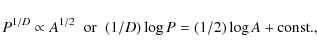 |
(4) |
where P is perimeter and A area of the elements. Self-similarity, or geometric similarity, is described by a linear function between
4.2 The relation between magnetic elements and continuum intensity
It is interesting to discuss the locations of the magnetic elements in the continuum image, i.e. whether they are located in granular or intergranular areas. Figure 10 demonstrates the continuum image of the black box region in Fig. 1 with the boundary of each magnetic element. The magnetic elements are usually located in intergranular spaces, although there are also some elements located in bright granules. We computed the continuum intensity at the locations of magnetic elements and pixels with three different automatic methods. The first three panels of Fig. 11 show that the brightness distribution at the locations of elements reaches peaks at 0.97, 0.97, and 0.98 with our method, downhill, and clumping, respectively. The fourth panel shows the distribution in units of pixels. The peak value is also 0.97. However, the distribution is smoother than the first three panels because the number of pixels is large enough. And the continuum intensity of all elements with our method takes values in intervals [0.82,1.19], while that of all pixels takes values in [0.78, 1.29]. The range of pixel values is wider than that of elements, because the continuum intensity of each element take all the values in the element into consideration. However, the distributions are similar to each other.
![\begin{figure}
\par\includegraphics[width=9cm,clip]{10946fig10.eps}
\end{figure}](/articles/aa/full_html/2009/38/aa10946-08/img57.png) |
Figure 10: Black box subfield of continuum image overplotted by the boundary of each magnetic element. |
| Open with DEXTER | |
| |
Figure 11: Brightness distribution at the locations of magnetic elements and pixels with the three different methods. Panel 1: brightness distribution at the locations of magnetic elements with the marker-controlled watershed method. Panel 2: brightness distribution at the locations of elements with downhill. Panel 3: brightness distribution at the locations of elements using clumping. Panel 4: brightness distribution in units of pixels in the longitudinal magnetogram. |
| Open with DEXTER | |
| |
Figure 12: Brightness vs. flux density at the location of each element and pixel with the three different methods. Panel 1: brightness vs. flux density of the longitudinal magnetic elements with the marker-controlled watershed method. Panel 2: brightness vs. flux density of elements found by downhill. Panel 3: brightness vs. flux density of elements using clumping. Panel 4: brightness vs. flux density of the longitudinal magnetic pixels. |
| Open with DEXTER | |
Figure 12 shows the relation between the continuum intensity and magnetic field strength at locations of elements and pixels with three different automatic methods. The first three panels of Fig. 12 show that the range of continuum intensity gets narrower with the increase in magnetic flux density. However, the ranges of flux density are different with different methods. The ranges are [0 G, 646 G], [0 G, 887 G], and [0 G, 162 G] with our method, downhill, and clumping, respectively. The first two panels show that the continuum intensity is around 1 when the flux density is higher than 100 G with marker-controlled watershed and downhill. With clumping, the continuum intensity is around 1 when the flux density is higher than 30 G. The fourth panel gives the relation between continuum intensity and flux density in units of pixels. There is a wide spread compared with the trend. When the flux density is in the range [400 G, 900 G], some elements are located at intergranular lanes, and others at bright granules. If the flux density is higher than 900 G or lower than 400 G, the elements prefer to locate at intergranular lanes. The magnetic field strength of magnetic elements is between 0 and 646 G, and the continuum intensity of these elements is between 0.82 and 1.19. While the range of magnetic flux density in units of pixels is between 0 and 1315 G. And the continuum intensity of these pixels is between 0.78 and 1.29.
The range for pixels is wider than for elements because each element
includes strong pixels as the center, and weak pixels as the
boundary. Similarly, the range in continuum intensity of pixels is
wider than that of elements. However, we can get almost the same
trend in these two cases. With the increase in the flux density, the
range in continuum intensity decreases. And the continuum intensity
is the median in the areas where the flux density is strong. We can
also find some differences in these cases. As for magnetic elements,
a large part of the weak elements are located in the areas with
relative continuum intensity ![]() 1.0, while weak elements in the
areas with relative continuum intensity <1.0 also exist. As for
pixels, the number of weak elements located in the areas with
relative continuum intensity
1.0, while weak elements in the
areas with relative continuum intensity <1.0 also exist. As for
pixels, the number of weak elements located in the areas with
relative continuum intensity ![]() 1.0 is almost the same as that
located at areas with relative continuum intensity <1.0.
1.0 is almost the same as that
located at areas with relative continuum intensity <1.0.
![\begin{figure}
\par\includegraphics[width=9cm,clip]{10946fig13.eps}
\end{figure}](/articles/aa/full_html/2009/38/aa10946-08/img60.png) |
Figure 13: Black box subfield of Dopplergram overplotted by the boundary of each magnetic element. |
| Open with DEXTER | |
![\begin{figure}
\par\includegraphics[width=18cm,clip]{10946fig14.eps}
\end{figure}](/articles/aa/full_html/2009/38/aa10946-08/img61.png) |
Figure 14: The distribution of Doppler velocity and the relation between Doppler velocity and magnetic flux density with the three different methods. ME is short for magnetic elements. The panels in the first row are the results with the marker-controlled watershed method. The panels in the second and third rows are with downhill and clumping, respectively. The first column shows the distribution of absolute mean Doppler velocity in units of magnetic elements. The second column shows the relation between absolute mean Doppler velocity and flux density of elements. The third and fourth columns use the positive and negative Doppler velocities of each element, separately. |
| Open with DEXTER | |
4.3 The relation between magnetic elements and Doppler velocity
Figure 13 shows only the black box region of the Dopplergram in Fig. 1 and this region is over-plotted by the boundary of all magnetic elements. It is easy to see that the magnetic elements are usually located in downflows, and a few magnetic elements locate in upflows. Figure 14 shows the distribution of Doppler velocity and the relation between Doppler velocity and magnetic flux density with the three different methods. The panels in the first row are the results with the marker-controlled watershed method, and the panels in the second and third rows are with downhill and clumping, respectively. This figure shows that the trends are similar with the three different methods. The absolute velocity distribution at the locations of magnetic elements with our method arrives at the peak value when the velocity is 1.00 km s-1, while the peak values are 0.76 km s-1 with downhill and 1.02 km s-1with clumping. From the three panels of the second column, we know that the rules are similar with the three different methods. Strongly magnetized regions only have weak absolute Doppler velocities. With our method, the majority of weak magnetic elements locate at the areas where the velocity is above 1.00 km s-1, however we can find that there are also weak magnetic elements at the location of low velocity. The absolute velocity is lower than 1.00 km s-1 in the regions where the magnetic flux density of elements is larger than 100 G. We also computed the mean Doppler velocity of elements and find that 67.7% of elements have positive mean Doppler velocity.
We computed the upflows and downflows at the locations of magnetic elements, respectively, shown in the third and fourth columns of Fig. 14 with the three different methods. The rules are also similar to each other. The distribution of upflows and downflows is not symmetrical in the third column. With our method, there is an ascending trend in the interval where the positive Doppler velocity is greater than 0.2 km s-1 and less than 1.00 km s-1. The fourth column shows that the positive and negative Doppler velocities are below 1.00 km s-1 in the regions where the flux density is higher than 100 G.
5 Conclusions and discussion
In this work we employed a mark-controlled watershed method to detect magnetic elements automatically and to explore properties of magnetic elements in quiet Sun. We used the magnetogram, the continuum image, and the Doppler image on April 16, 2007 taken by SOT instrument aboard HINODE. Our method identified 10279 magnetic elements. Compared with the other two automatic detection methods, downhill and clumping, the number of magnetic elements identified by our method is the median.
The magnetic flux density of all elements takes values from 0 to 646 G. The log-log magnetic flux distribution reaches
only one peak at
![]() Mx for the whole region. This
conclusion is different from Wang et al. (1995), who found that the
distribution of network and IN fluxes show two peaks using
observations made by BBSO. And we found that the smallest element is
Mx for the whole region. This
conclusion is different from Wang et al. (1995), who found that the
distribution of network and IN fluxes show two peaks using
observations made by BBSO. And we found that the smallest element is
![]() Mx, far smaller than the 1016 Mx found
by Parnell et al. (2008) in SOT/Hinode, because we analyzed the
pixels with total polarization degree above one times the noise
level
Mx, far smaller than the 1016 Mx found
by Parnell et al. (2008) in SOT/Hinode, because we analyzed the
pixels with total polarization degree above one times the noise
level
![]() Ic in the polarization continuum.
Ic in the polarization continuum.
The fractal dimension of our observations is
![]() for a
pixel corresponding to 0
for a
pixel corresponding to 0
![]() 16. This result agrees with
previous results (Criscuoli et al. 2007; Janßen et al. 2003). In our
work, the relative continuum intensity distribution at the locations
of magnetic elements reaches a peak at 0.97, which shows that many
magnetic elements located in the areas where the relative continuum
intensity are lower than the average continuum intensity. The
distribution of magnetic elements is similar to that of pixels. And
the distribution of the pixels is consistent with
Stolpe & Kneer (2000) and Hartje & Kneer (2002). The relative
continuum intensity histogram is centered on the value less than
1.00. And a trend exists toward lower intensities with increasing
magnetic flux amplitude.
16. This result agrees with
previous results (Criscuoli et al. 2007; Janßen et al. 2003). In our
work, the relative continuum intensity distribution at the locations
of magnetic elements reaches a peak at 0.97, which shows that many
magnetic elements located in the areas where the relative continuum
intensity are lower than the average continuum intensity. The
distribution of magnetic elements is similar to that of pixels. And
the distribution of the pixels is consistent with
Stolpe & Kneer (2000) and Hartje & Kneer (2002). The relative
continuum intensity histogram is centered on the value less than
1.00. And a trend exists toward lower intensities with increasing
magnetic flux amplitude.
The relative continuum intensity at the locations of magnetic elements from our observations is between 0.82 and 1.19. Its range decreases with an increase in the flux density. The strong magnetic elements are located at the granulation boundary. And we found that the relation between flux density and relative continuum intensity in units of pixels is consistent with Title et al. (1987). The strong magnetic fields are also located at the granulation boundary. We see that weak magnetic fields in units of pixels are located in the areas with diversified relative continuum intensity, and most of them have a relative continuum intensity less than 1.0. This conclusion is consistent with Stolpe & Kneer (2000). Likewise, we also found that the relative continuum intensity is around 1.0 in the areas where flux density of magnetic elements is higher than 150 G. While for the areas where flux density in units of pixels is from 300 G to 1000 G, the relative continuum intensity increases from 0.9 to 1.1. And it decreases from 1.1 to 0.9 above 1000 G.
Stolpe & Kneer (2000) find that the low magnetic flux structures do
not show a preferred sign of velocity. The structures with higher
flux tend to be located in downflow areas. We computed the Doppler
velocity at the locations of magnetic elements where both upflows
and downflows exist. The absolute velocity is high in the areas of a
majority of weak magnetic elements, while the low velocity also
exists in these areas. The absolute velocity is below 1 km s-1 in
the regions where the magnetic flux density of elements is higher
than 100 G. This shows that strongly magnetized regions only have
weak absolute Doppler velocities, which may be a sign of convective
suppression by the strong magnetic elements. The energy balance
between the convection and the magnetic field is achieved at around
700 G, depending on what numbers one uses for the density at the
![]() surface and for the convective turnover speed; hence,
convective suppression is to be expected. But this is a nice result
that is at odds with the conventional picture
(Berger & Title 1996; Berger et al. 1995; Simon et al. 2001) that flux
concentrations should be found at downflow sites and small flux
fragments having intense fields of around 1500 G are confined
mainly to intergranular lanes (Berger & Title 1996; Berger et al. 1995).
In contrast to the above dimensionality and size distribution
results, this appears rather strong, since the scatter plot in the
second row of Fig. 14 shows essentially
no strong downflows in the presence of strong magnetic elements.
surface and for the convective turnover speed; hence,
convective suppression is to be expected. But this is a nice result
that is at odds with the conventional picture
(Berger & Title 1996; Berger et al. 1995; Simon et al. 2001) that flux
concentrations should be found at downflow sites and small flux
fragments having intense fields of around 1500 G are confined
mainly to intergranular lanes (Berger & Title 1996; Berger et al. 1995).
In contrast to the above dimensionality and size distribution
results, this appears rather strong, since the scatter plot in the
second row of Fig. 14 shows essentially
no strong downflows in the presence of strong magnetic elements.
Acknowledgements
We are grateful to the HINODE team for providing the data. HINODE is a Japanese mission developed and launched by ISAS/JAXA, with NAOJ as domestic partner and NASA and STFC (UK) as international partners. It is operated by these agencies in co-coperation with ESA and NSC (Norway). We also thank Prof. Jingxiu Wang for his constructive comments, and thank Dr. Derek Lamb for providing his codes of SWAMIS. The work is supported by the National Outstanding Youth Foundation of China, the Cheung Kong Scholars Programme of China, and the National Natural Science Foundation of China under Grants No. 60703013 and 10978011.
References
- Berger, T., & Title, A. 1996, ApJ, 463, 365 [NASA ADS] [CrossRef]
- Berger, T., Schrijver, C., Shine, R., & Tarbell, T. 1995, ApJ, 454, 531 [NASA ADS] [CrossRef]
- Beucher, S., & Meyer, F. 1993, Mathematical Morphology in Image Processing, 34, 433
- Courses, E., & Surveys, T. 1999, IEEE Transactions on Image Processing, 8, 69 [CrossRef]
- Criscuoli, S., Rast, M., Ermolli, I., & Centrone, M. 2007, A&A, 461, 331 [NASA ADS] [CrossRef] [EDP Sciences]
- DeForest, C., Hagenaar, H., Lamb, D., Parnell, C., & Welsch, B. 2007, ApJ, 666, 576 [NASA ADS] [CrossRef] (In the text)
- Domínguez Cerdeña, I., Kneer, F., & Almeida, J. 2003, ApJ, 582, 55 [NASA ADS] [CrossRef]
- Domínguez Cerdeña, I., Almeida, J., & Kneer, F. 2006, ApJ, 636, 496 [NASA ADS] [CrossRef]
- Hagenaar, H. 2001, ApJ, 555, 448 [NASA ADS] [CrossRef]
- Hagenaar, H., Schrijver, C., Title, A., & Shine, R. 1999, ApJ, 511, 932 [NASA ADS] [CrossRef]
- Handy, B., Acton, L., Kankelborg, C., et al. 1999, Sol. Phys., 187, 229 [NASA ADS] [CrossRef] (In the text)
- Haris, K., Efstratiadis, S., Maglaveras, N., & Katsaggelos, A. 1998, IEEE Transactions on Image Processing, 7, 1684 [NASA ADS] [CrossRef]
- Hartje, B., & Kneer, F. 2002, A&A, 385, 264 [NASA ADS] [CrossRef] [EDP Sciences] (In the text)
- Harvey, K., & Martin, S. 1973, Sol. Phys., 32, 389 [NASA ADS] [CrossRef] (In the text)
- Harvey, J., Branston, D., Henney, C., & Keller, C. 2007, ApJ, 659, 177 [NASA ADS] [CrossRef]
- Harvey-Angle, K. 1993, Ph.D. Thesis, University of Utrecht (In the text)
- Ichimoto, K., Lites, B., Elmore, D., et al. 2008, Sol. Phys., 249, 233 [NASA ADS] [CrossRef]
- Janßen, K., Vogler, A., & Kneer, F. 2003, A&A, 409, 1127 [NASA ADS] [CrossRef] [EDP Sciences]
- Keller, C. 1992, Nature, 359, 307 [NASA ADS] [CrossRef]
- Keller, C., Deubner, F., Egger, U., Fleck, B., & Povel, H. 1994, A&A, 286, 626 [NASA ADS] (In the text)
- Kosugi, T., Matsuzaki, K., Sakao, T., et al. 2007, Sol. Phys., 243, 3 [NASA ADS] [CrossRef] (In the text)
- Lamb, D., & Deforest, C. 2003, AGU, B530 (In the text)
- Leibacher, J. 1999, Adv. Space Res., 24, 173 [NASA ADS] [CrossRef] (In the text)
- Leighton, R., Noyes, R., & Simon, G. 1962, ApJ, 135, 474 [NASA ADS] [CrossRef] (In the text)
- Lin, H. 1995, ApJ, 446, 421 [NASA ADS] [CrossRef] (In the text)
- Lin, H., & Rimmele, T. 1999, ApJ, 514, 448 [NASA ADS] [CrossRef] (In the text)
- Lites, B., Elmore, D., Streander, K., et al. 2001, Proc. SPIE, 4498, 73 [NASA ADS] (In the text)
- Lites, B., & Socas-Navarro, H. 2004, ApJ, 613, 600 [NASA ADS] [CrossRef]
- Lites, B., Kubo, M., Socas-Navarro, H., et al. 2008, ApJ, 672, 1237 [NASA ADS] [CrossRef]
- Liu, Y., Zhang, H., Ai, G., Wang, H., & Zirin, H. 1994, A&A, 283, 215 [NASA ADS]
- Livingston, W., & Harvey, J. 1975, BAAS, 7, 346 [NASA ADS]
- Mandelbrot, B. 1982, The Fractal Geometry of Nature (WH Freeman)
- Meyer, F., & Beucher, S. 1990, Journal of Visual Communication and Image Representation, 1, 21 [CrossRef] (In the text)
- Parnell, C. 2002, MNRAS, 335, 389 [NASA ADS] [CrossRef] (In the text)
- Parnell, C., Deforest, C., Hagenaar, H., Lamb, D., & Welsch, B. 2008, PASP, 397, 31 (In the text)
- Rezaei, R., Schlichenmaier, R., Beck, C., Bruls, J., & Schmidt, W. 2007a, A&A, 466, 1131 [NASA ADS] [CrossRef] [EDP Sciences] (In the text)
- Rezaei, R., Steiner, O., Wedemeyer-Böhm, S., et al. 2007b, A&A, 476, 33 [NASA ADS] [CrossRef]
- Rivest, J., Soille, P., & Beucher, S. 2005, Proc. SPIE, 1658, 139 (In the text)
- Salembier, P., & Pardas, M. 1994, IEEE Transactions on Image Processing, 3, 639 [NASA ADS] [CrossRef]
- Salembier, P., & Marques, F. 1999, IEEE Transactions on Circuits and Systems for Video Technology, 9, 1147 [CrossRef]
- Sánchez Almeida, J. 2003, Solar wind ten, 679, 293 [NASA ADS]
- Sánchez Almeida, J. 2007, ApJ, 657, 1150 [NASA ADS] [CrossRef]
- Scherrer, P., Bogart, R., Bush, R., et al. 1995, Sol. Phys., 162, 129 [NASA ADS] [CrossRef] (In the text)
- Schrijver, C., & Title, A. 2003, ApJ, 597, 165 [NASA ADS] [CrossRef] (In the text)
- Schrijver, C., Title, A., van Ballegooijen, A., Hagenaar, H., & Shine, R. 1997, ApJ, 487, 424 [NASA ADS] [CrossRef]
- Shimizu, T., Nagata, S., Tsuneta, S., et al. 2008, Sol. Phys., 249, 221 [NASA ADS] [CrossRef]
- Simon, G., Title, A., & Weiss, N. 2001, ApJ, 561, 427 [NASA ADS] [CrossRef]
- Smithson, R. 1975, BAAS, 7, 346 [NASA ADS]
- Socas-Navarro, H., Martinez Pillet, V., & Lites, B. 2004, ApJ, 611, 1139 [NASA ADS] [CrossRef]
- Stolpe, F., & Kneer, F. 2000, A&A, 353, 1094 [NASA ADS] (In the text)
- Suarez, D., Rubio, L., del Toro Iniesta, J., et al. 2007, PASJ, 59, 837
- Suematsu, Y., Tsuneta, S., Ichimoto, K., et al. 2008, Sol. Phys., 249, 197 [NASA ADS] [CrossRef] (In the text)
- Title, A., Tarbell, T., & Topka, K. 1987, ApJ, 317, 892 [NASA ADS] [CrossRef] (In the text)
- Title, A., Topka, K., & Tarbell, T. 1992, ApJ, 369, 351 [NASA ADS]
- Tremeau, A., & Colantoni, P. 2000, IEEE Transactions on Image Processing, 9, 735 [NASA ADS] [CrossRef]
- Tsuneta, S., Ichimoto, K., Katsukawa, Y., et al. 2008, Sol. Phys., 249, 167 [NASA ADS] [CrossRef]
- Turner, M., Blackledge, J., & Andrews, P. 1998, Fractal Geometry in Digital Imaging (Academic Press) (In the text)
- Vincent, L. 1993, IEEE Transactions on Image Processing, 2, 176 [NASA ADS] [CrossRef] (In the text)
- Wang, H., Tang, F., Zirin, H., & Wang, J. 1996, Sol. Phys., 165, 223 [NASA ADS] [CrossRef] (In the text)
- Wang, J., Wang, H., Tang, F., Lee, J., & Zirin, H. 1995, Sol. Phys., 160, 277 [NASA ADS] [CrossRef] (In the text)
- Welsch, B., & Longcope, D. 2003, ApJ, 588, 620 [NASA ADS] [CrossRef] (In the text)
- Zhang, H., Scharmer, G., Lofdahl, M., & Yi, Z. 1998a, Sol. Phys., 183, 283 [NASA ADS] [CrossRef] (In the text)
- Zhang, J., Ma, J., & Wang, H. 2006, ApJ, 649, 464 [NASA ADS] [CrossRef]
- Zhang, J., Lin, G., Wang, J., Wang, H., & Zirin, H. 1998b, Sol. Phys., 178, 245 [NASA ADS] [CrossRef] (In the text)
- Zhang, J., Lin, G., Wang, J., Wang, H., & Zirin, H. 1998c, A&A, 338, 322 [NASA ADS]
- Zhang, J., Wang, J., Wang, H., & Zirin, H. 1998d, A&A, 335, 341 [NASA ADS]
All Tables
Table 1: Location information of pixels around the center of a magnetic element.
Table 2: Statistics of magnetic elements with the three different methods.
All Figures
| |
Figure 1:
Longitudinal magnetogram ( left), continuum image
( middle), and Dopplergram ( right) of a quiet Sun region obtained at
HINODE on April 16, 2007. The field of view is
147
|
| Open with DEXTER | |
| In the text | |
| |
Figure 2: Effectiveness of the marks. The first panel is a small part of the original magnetogram. The second panel is the topographic surface of the first panel region. The third panel shows the watershed results. The fourth panel illustrates the mark-controlled watershed results. |
| Open with DEXTER | |
| In the text | |
| |
Figure 3: Segmentation of magnetic elements. Image 1 is center, white rectangle region of magnetogram in Fig. 1. Image 2 is segmentation results. Image 3 marks the center of each magnetic element in the original magnetogram. Image 4 marks the boundary of each magnetic element in the original magnetogram. |
| Open with DEXTER | |
| In the text | |
| |
Figure 4: Results of different magnetic element detection methods. (1) White rectangle region of original magnetogram in Fig. 1. (2) Marker-controlled watershed. (3) Downhill identifies one magnetic element per local maximum region. (4) Clumping identifies all connected above-threshold pixels into a single magnetic element. |
| Open with DEXTER | |
| In the text | |
| |
Figure 5: Log-log magnetic flux distribution of positive and negative magnetic elements in the longitudinal magnetogram with three different automatic detection methods. The first panel is with the marker-controlled watershed, the second one with downhill, the third with clumping. |
| Open with DEXTER | |
| In the text | |
| |
Figure 6: Log-log area distribution of positive and negative magnetic elements in the longitudinal magnetogram using three different automatic detection methods. The first panel is with the marker-controlled watershed, the second with downhill, the third with clumping. |
| Open with DEXTER | |
| In the text | |
| |
Figure 7: Log-log magnetic flux density distribution of positive and negative magnetic elements in the longitudinal magnetogram with three different automatic detection methods. The first panel is with the marker-controlled watershed, the second with downhill, the third with clumping. |
| Open with DEXTER | |
| In the text | |
| |
Figure 8: Scatter plot of absolute flux versus area of each magnetic element. |
| Open with DEXTER | |
| In the text | |
| |
Figure 9:
Perimeter-area relation with the three different
automatic detection methods. The first panel is with the
marker-controlled watershed method. This method detects 10 279
magnetic elements giving the fractal dimension
|
| Open with DEXTER | |
| In the text | |
| |
Figure 10: Black box subfield of continuum image overplotted by the boundary of each magnetic element. |
| Open with DEXTER | |
| In the text | |
| |
Figure 11: Brightness distribution at the locations of magnetic elements and pixels with the three different methods. Panel 1: brightness distribution at the locations of magnetic elements with the marker-controlled watershed method. Panel 2: brightness distribution at the locations of elements with downhill. Panel 3: brightness distribution at the locations of elements using clumping. Panel 4: brightness distribution in units of pixels in the longitudinal magnetogram. |
| Open with DEXTER | |
| In the text | |
| |
Figure 12: Brightness vs. flux density at the location of each element and pixel with the three different methods. Panel 1: brightness vs. flux density of the longitudinal magnetic elements with the marker-controlled watershed method. Panel 2: brightness vs. flux density of elements found by downhill. Panel 3: brightness vs. flux density of elements using clumping. Panel 4: brightness vs. flux density of the longitudinal magnetic pixels. |
| Open with DEXTER | |
| In the text | |
| |
Figure 13: Black box subfield of Dopplergram overplotted by the boundary of each magnetic element. |
| Open with DEXTER | |
| In the text | |
| |
Figure 14: The distribution of Doppler velocity and the relation between Doppler velocity and magnetic flux density with the three different methods. ME is short for magnetic elements. The panels in the first row are the results with the marker-controlled watershed method. The panels in the second and third rows are with downhill and clumping, respectively. The first column shows the distribution of absolute mean Doppler velocity in units of magnetic elements. The second column shows the relation between absolute mean Doppler velocity and flux density of elements. The third and fourth columns use the positive and negative Doppler velocities of each element, separately. |
| Open with DEXTER | |
| In the text | |
Copyright ESO 2009
Current usage metrics show cumulative count of Article Views (full-text article views including HTML views, PDF and ePub downloads, according to the available data) and Abstracts Views on Vision4Press platform.
Data correspond to usage on the plateform after 2015. The current usage metrics is available 48-96 hours after online publication and is updated daily on week days.
Initial download of the metrics may take a while.