| Issue |
A&A
Volume 505, Number 2, October II 2009
|
|
|---|---|---|
| Page(s) | 483 - 495 | |
| Section | Extragalactic astronomy | |
| DOI | https://doi.org/10.1051/0004-6361/200810320 | |
| Published online | 11 August 2009 | |
The age of blue LSB galaxies
E. I. Vorobyov1,2 - Yu. Shchekinov5,![]() - D. Bizyaev3,4 - D. Bomans5 - R.-J. Dettmar5
- D. Bizyaev3,4 - D. Bomans5 - R.-J. Dettmar5
1 - The Institute for Computational Astrophysics, Saint Mary's University, Halifax NS,
B3H 3C3, Canada
2 -
Institute of Physics, South Federal University, Stachki 194, Rostov-on-Don, Russia
3 -
New Mexico State University/APO, Sunspot, NM, 88349, USA
4 -
Sternberg Astronomical Institute, Universitetsky 13, Moscow 119992, Russia
5 -
Astronomisches Institut, Ruhr-Universität Bochum, Bochum, Germany
Received 3 June 2009 / Accepted 15 June 2009
Abstract
Context. Low metallicities, high gas-to-star mass ratios, and blue colors of most low surface brightness (LSB) galaxies imply that these systems may be younger than their high surface brightness counterparts.
Aims. We look for observational signatures that can help to constrain the age of blue LSB galaxies.
Methods. We use numerical hydrodynamic modelling to study the long-term (![]() 13 Gyr) dynamical and chemical evolution of blue LSB galaxies, adopting a sporadic scenario of star formation. Our model galaxy consists of a thin gas disk, a stellar disk with a developed spiral structure and a spherical dark matter halo. Our models utilize various rates of star formation and different shapes of the initial mass function (IMF). We complement hydrodynamic modelling with population synthesis modelling to produce the integrated B-V colors and H
13 Gyr) dynamical and chemical evolution of blue LSB galaxies, adopting a sporadic scenario of star formation. Our model galaxy consists of a thin gas disk, a stellar disk with a developed spiral structure and a spherical dark matter halo. Our models utilize various rates of star formation and different shapes of the initial mass function (IMF). We complement hydrodynamic modelling with population synthesis modelling to produce the integrated B-V colors and H![]() equivalent widths.
equivalent widths.
Results. We find that the mean oxygen abundances, B-V colors, H![]() equivalent widths, and the radial fluctuations in the oxygen abundance, when considered altogether, can be used to constrain the age of blue LSB galaxies if some independent knowledge of the IMF is available. Our modelling strongly suggests the existence of a minimum age for blue LSB galaxies. Model B-V colors and mean oxygen abundances set a tentative minimum age at 1.5-3.0 Gyr, whereas model H
equivalent widths, and the radial fluctuations in the oxygen abundance, when considered altogether, can be used to constrain the age of blue LSB galaxies if some independent knowledge of the IMF is available. Our modelling strongly suggests the existence of a minimum age for blue LSB galaxies. Model B-V colors and mean oxygen abundances set a tentative minimum age at 1.5-3.0 Gyr, whereas model H![]() equivalent widths suggest a larger value of the order of 5-6 Gyr. The latter value may decrease somewhat if blue LSB galaxies host IMFs with a truncated upper mass limit. We found no firm evidence that the age of blue LSB galaxies is significantly lower than 13 Gyr.
equivalent widths suggest a larger value of the order of 5-6 Gyr. The latter value may decrease somewhat if blue LSB galaxies host IMFs with a truncated upper mass limit. We found no firm evidence that the age of blue LSB galaxies is significantly lower than 13 Gyr.
Conclusions. The age of blue LSB galaxies may vary between 1.5-6 Gyr and 13 Gyr, depending on the physical conditions in the disk that control the form of the IMF and the rate of star formation. A failure to observationally detect large radial fluctuations in the oxygen abundance of the order of 0.5-1.0 dex, which, according to our modelling, are characteristic of (1-2)-Gyr-old galaxies, will argue in favour of the more evolved nature of blue LSB galaxies.
Key words: ISM: abundances - galaxies: abundances - galaxies: evolution
1 Introduction
Low surface brightness (LSB) galaxies have a central surface brightness much
fainter than the Freeman value
![]() mag arcsec-2.
These galaxies are thought to represent a significant fraction of the galaxy number density
in the universe (Trachternach et al. 2006; O'Neil & Bothun 2000; McGaugh et al. 1995a). LSB galaxies show a wide spread of
colours ranging from red (
mag arcsec-2.
These galaxies are thought to represent a significant fraction of the galaxy number density
in the universe (Trachternach et al. 2006; O'Neil & Bothun 2000; McGaugh et al. 1995a). LSB galaxies show a wide spread of
colours ranging from red (
![]() )
to very blue (
)
to very blue (
![]() )
(O'Neil et al. 1997),
but the most common type seems to be blue LSB galaxies: late-type, disk dominated spirals with central
surface brightness
)
(O'Neil et al. 1997),
but the most common type seems to be blue LSB galaxies: late-type, disk dominated spirals with central
surface brightness
![]() mag arcsec-2 and colors lying in the range
(B-V)=0.3-0.7.
These blue LSB galaxies are among the most gas-rich (up to 50% of the total baryonic mass)
and metal-deficient (about 5-20% of the solar metallicity) galaxies
(de Blok & van der Hulst 1998; Kuzio de Narray et al. 2004; McGaugh & Blok 1997; Rönnback & Bergvall 1995; McGaugh 1994).
mag arcsec-2 and colors lying in the range
(B-V)=0.3-0.7.
These blue LSB galaxies are among the most gas-rich (up to 50% of the total baryonic mass)
and metal-deficient (about 5-20% of the solar metallicity) galaxies
(de Blok & van der Hulst 1998; Kuzio de Narray et al. 2004; McGaugh & Blok 1997; Rönnback & Bergvall 1995; McGaugh 1994).
Low metallicities and large gas-to-star mass ratios may be interpreted in various ways.
For instance, blue LSB galaxies may have formed recently, at redshifts close to
z=0. However, this can contradict the hierarchical scenario of large-scale structure
formation, within which low-mass galaxies form first at redshifts close
to the onset of the reionization epoch, ![]() .
Therefore, it is more likely that
blue LSB galaxies have formed at large z but have had a delayed onset of the major
star formation epoch. In this case, conflict with the hierarchical structure formation is relaxed.
Indeed, blue LSB galaxies show a wide range of masses with
an excess of dwarf systems with luminosities of the order of
.
Therefore, it is more likely that
blue LSB galaxies have formed at large z but have had a delayed onset of the major
star formation epoch. In this case, conflict with the hierarchical structure formation is relaxed.
Indeed, blue LSB galaxies show a wide range of masses with
an excess of dwarf systems with luminosities of the order of
![]() (Sprayberry et al. 1997).
Such dwarf systems are known to have a younger mean stellar age than their more massive
counterparts - a phenomenon known as ``downsizing'' (e.g. Thomas et al. 2005).
Another possible interpretation of the apparent unevolved nature of blue LSBs is that
they do not form late, nor have a delayed onset of star formation, but simply evolve
slower than their high surface brightness counterparts (e.g. van den Hoek et al. 2000).
(Sprayberry et al. 1997).
Such dwarf systems are known to have a younger mean stellar age than their more massive
counterparts - a phenomenon known as ``downsizing'' (e.g. Thomas et al. 2005).
Another possible interpretation of the apparent unevolved nature of blue LSBs is that
they do not form late, nor have a delayed onset of star formation, but simply evolve
slower than their high surface brightness counterparts (e.g. van den Hoek et al. 2000).
There have been many efforts to infer the age of blue LSB galaxies from
the properties of stellar populations.
Broadband photometric studies, complemented by H![]() emission line data
and synthetic stellar population code modeling, predict quite a wide range for the ages of
blue LSB galaxies: from 1-2 Gyr (Zackrisson et al. 2005) to 7-9 Gyr (Padoan et al. 1997; Jimenez et al. 1998).
Rather young ages of blue LSB galaxies (<5 Gyr) follow also from their (V-I) colors
and HI content (Schombert et al. 2001). The comparison of measured spectral energy distributions in a sample
of LSB galaxies with synthetic spectra (derived assuming an exponentially declining
SFR) by Haberzettl et al. (2005) suggests the ages of the dominant stellar population
to be between 2 and 5 Gyr.
emission line data
and synthetic stellar population code modeling, predict quite a wide range for the ages of
blue LSB galaxies: from 1-2 Gyr (Zackrisson et al. 2005) to 7-9 Gyr (Padoan et al. 1997; Jimenez et al. 1998).
Rather young ages of blue LSB galaxies (<5 Gyr) follow also from their (V-I) colors
and HI content (Schombert et al. 2001). The comparison of measured spectral energy distributions in a sample
of LSB galaxies with synthetic spectra (derived assuming an exponentially declining
SFR) by Haberzettl et al. (2005) suggests the ages of the dominant stellar population
to be between 2 and 5 Gyr.
In this paper, we perform numerical hydrodynamic modelling of the dynamical,
chemical, and photometric evolution of blue LSB galaxies to constrain
their typical range of ages.
The cornerstone supposition of our modelling, motivated by observational evidence,
is the sporadic nature of star formation in blue LSB galaxies.
Indeed, McGaugh (1994), de Blok et al. (1995), Gerretsen & de Blok (1999), and others argue that
the primary cause of the blue colors is the young age of the dominant stellar
population. This can take the form of young local bursts of star formation superimposed (or not)
on a continuous low-rate star formation. Available H![]() images of LSB galaxies
(see e.g. McGaugh et al. 1995b; Auld et al. 2006; McGaugh & Bothun 1994) appear to support this so-called sporadic star formation
scenario. Current star formation is localized to a handful of
compact regions. There is little or no diffuse H
images of LSB galaxies
(see e.g. McGaugh et al. 1995b; Auld et al. 2006; McGaugh & Bothun 1994) appear to support this so-called sporadic star formation
scenario. Current star formation is localized to a handful of
compact regions. There is little or no diffuse H![]() emission coming
from the rest of the galactic disk. Randomly distributed star formation sites, along with
inefficient spatial stirring of heavy elements, give rise to radial fluctuations
in the oxygen abundance on spatial scales of the order of 1-2 kpc. The resulting
fluctuation spectrum is age-sensitive and can be potentially used to set order-of-magnitude
constraints on the age of blue LSB galaxies.
However, the age prediction may be considerably improved by using the mean oxygen abundances and H
emission coming
from the rest of the galactic disk. Randomly distributed star formation sites, along with
inefficient spatial stirring of heavy elements, give rise to radial fluctuations
in the oxygen abundance on spatial scales of the order of 1-2 kpc. The resulting
fluctuation spectrum is age-sensitive and can be potentially used to set order-of-magnitude
constraints on the age of blue LSB galaxies.
However, the age prediction may be considerably improved by using the mean oxygen abundances and H![]() equivalent widths provided that some independent knowledge of the initial mass function is available.
equivalent widths provided that some independent knowledge of the initial mass function is available.
This paper is organized as follows. In the next section we discuss qualitatively the processes that mix heavy elements in disks of LSB galaxies. Section 3 details our theoretical model, while Sect. 4 describes our observations. In Sects. 5 and 6 we discuss our numerical results, and Sect. 7 presents our main conclusions.
2 Mixing of heavy elements in LSB disks
In high surface brightness
(HSB) galaxies, mixing of heavy elements is provided by multiple shock waves from
supernova explosions. It requires approximately 100 Myr to homogenize
heavy elements in the warm neutral interstellar medium of HSB galaxies (de Avillez & MacLow 2002). LSB
galaxies, on the other hand, are characterized by a star formation rate (
![]() yr-1) that is almost two orders of magnitude lower than the Milky Way value,
yr-1) that is almost two orders of magnitude lower than the Milky Way value,
![]() yr-1. Consequently, the frequency of shock waves in the
interstellar medium of LSB galaxies and the
corresponding volume filling factor occupied by the shock processed gas
can be as small as
yr-1. Consequently, the frequency of shock waves in the
interstellar medium of LSB galaxies and the
corresponding volume filling factor occupied by the shock processed gas
can be as small as
![]() and
and
![]() ,
respectively. For comparison, the corresponding values
in the Milky Way are
,
respectively. For comparison, the corresponding values
in the Milky Way are
![]() (Draine & Salpeter 1979) and
(Draine & Salpeter 1979) and
![]() (de Avillez & Breitschwerdt 2005).
In these conditions, homogenization of heavy elements in
LSB galaxies may require a considerably longer time scale than 100 Myr, a typical value for
HSB galaxies. Differential rotation
of the galactic disk and radial convection driven by the spiral stellar
density waves may in principle be efficient in mixing of heavy elements
in LSB galaxies. However, the time scales for these processes in LSB galaxies
are not well known and numerical simulations are needed to determine their importance.
Therefore, the distribution
of heavy elements in the disk of an LSB galaxy may be characterized by
radial variations, the typical amplitude of which is expected to diminish with time.
It is our purpose to determine whether these radial abundance fluctuations
can be used to constrain the ages of LSB galaxies.
(de Avillez & Breitschwerdt 2005).
In these conditions, homogenization of heavy elements in
LSB galaxies may require a considerably longer time scale than 100 Myr, a typical value for
HSB galaxies. Differential rotation
of the galactic disk and radial convection driven by the spiral stellar
density waves may in principle be efficient in mixing of heavy elements
in LSB galaxies. However, the time scales for these processes in LSB galaxies
are not well known and numerical simulations are needed to determine their importance.
Therefore, the distribution
of heavy elements in the disk of an LSB galaxy may be characterized by
radial variations, the typical amplitude of which is expected to diminish with time.
It is our purpose to determine whether these radial abundance fluctuations
can be used to constrain the ages of LSB galaxies.
We note that mixing in the azimuthal direction is strongly enhanced by
differential rotation. The size of a mixing eddy grows with time
due to differential rotation as
![]() ,
much faster than due to hydrodynamic
mixing
,
much faster than due to hydrodynamic
mixing
![]() (Scalo & Elmegreen 2004), where
(Scalo & Elmegreen 2004), where
![]() is the radial derivative of
the rotation velocity, D is the diffusion coefficient. Differential rotation therefore
homogenizes metals in the azimuthal direction faster than in the radial one and the radial
variations remain for a longer time.
is the radial derivative of
the rotation velocity, D is the diffusion coefficient. Differential rotation therefore
homogenizes metals in the azimuthal direction faster than in the radial one and the radial
variations remain for a longer time.
3 Model LSB galaxy
3.1 Initial configuration
LSB galaxies show a wide range of morphological types, ranging from giant spirals to
dwarf irregular galaxies, from early-type red galaxies to late-type blue ones.
In this paper we focus on late-type blue LSB galaxies.
According to the observational data (van den Hoek et al. 2000), a typical blue LSB galaxy has a
dynamical mass of the order of
![]() and HI mass of the order of
and HI mass of the order of
![]() .
We closely follow these estimates when constructing our model galaxy.
Our model LSB galaxy consists of a thin gas disk, which evolves in the external
gravitational potential of both the spherical dark matter halo and extended stellar disk.
LSB galaxies often feature a few ill-defined spiral arms. Therefore, we assume that our model
stellar disk has developed a two-armed spiral structure. Below, we provide a more
detailed explanation for each of the constituents of our model galaxy.
.
We closely follow these estimates when constructing our model galaxy.
Our model LSB galaxy consists of a thin gas disk, which evolves in the external
gravitational potential of both the spherical dark matter halo and extended stellar disk.
LSB galaxies often feature a few ill-defined spiral arms. Therefore, we assume that our model
stellar disk has developed a two-armed spiral structure. Below, we provide a more
detailed explanation for each of the constituents of our model galaxy.
The velocity field of most LSB galaxies is better fitted by dark matter models described by
a modified isothermal sphere rather than by a NFW profile (Kuzio de Naray et al. 2006). Therefore,
the spherical dark matter halo in our model is modelled by a radial density profile described by
the modified isothermal sphere
where
![\begin{displaymath}{\partial \Phi_{\rm h} \over \partial r}=4 \pi G \rho_{\rm h0...
...n(r/r_{\rm h}) \right]
\left({r_{\rm h}\over r}\right)^2 \cdot
\end{displaymath}](/articles/aa/full_html/2009/38/aa10320-08/img33.png)
The stellar component of our model galaxy consists of two parts - an axisymmetric stellar disk and a two-armed spiral pattern. The former is described by a radially declining exponential profile
where
![\begin{displaymath}\Phi_{\rm st}(r,z=0)= - \pi G \Sigma_{\rm s0} r \left[I_0(y) K_1(y) - I_1(y) K_0(y) \right],
\end{displaymath}](/articles/aa/full_html/2009/38/aa10320-08/img39.png) |
(4) |
where In and Kn are modified Bessel functions of the first and second kinds, respectively, and
The non-axisymmetric gravitational potential of stellar spiral arms is described in
polar coordinates (![]() )
by a running density wave (see
e.g. Vorobyov & Shchekinov 2005)
)
by a running density wave (see
e.g. Vorobyov & Shchekinov 2005)
![\begin{displaymath}\Phi_{\rm sp}(r,\phi)=-C(r) \cos\left[ m(\cot(i) \ln(r/r_{\rm sp})+\phi - \Omega_{\rm sp} t)\right],
\end{displaymath}](/articles/aa/full_html/2009/38/aa10320-08/img42.png)
where C(r) is the radially varying amplitude, i is the pitch angle,
The amplitude C(r) of the spiral stellar gravitational potential
![]() determines the response
of the gas and consequently the appearance of a spiral pattern in the gas disk.
We adopt the following expression for the amplitude
determines the response
of the gas and consequently the appearance of a spiral pattern in the gas disk.
We adopt the following expression for the amplitude
![]() .
Here, C0(r) is a linear function of radius which has a value of 0 at r=0 kpc and
equals
.
Here, C0(r) is a linear function of radius which has a value of 0 at r=0 kpc and
equals
![]() (in dimensionless units) at r=17 kpc. The amplitude is set to zero at the galactic
center to ensure that the gravitational potential of the stellar spiral density wave diminishes
at small galactocentric distances.
Otherwise, even a small-amplitude spiral gravitational potential would produce
strong azimuthal gravitational forces near the galactic center due to
converging radial gridlines in polar coordinates, which quickly destroys the gas disk during
the numerical simulations.
The exponent
(in dimensionless units) at r=17 kpc. The amplitude is set to zero at the galactic
center to ensure that the gravitational potential of the stellar spiral density wave diminishes
at small galactocentric distances.
Otherwise, even a small-amplitude spiral gravitational potential would produce
strong azimuthal gravitational forces near the galactic center due to
converging radial gridlines in polar coordinates, which quickly destroys the gas disk during
the numerical simulations.
The exponent ![]() decreases linearly with radius r. More specifically,
we choose
decreases linearly with radius r. More specifically,
we choose
![]() ,
and
,
and
![]() .
This specific form of C(r) allows us to produce spiral gravitational
potentials with different shapes and maximum amplitudes.
The resulting ratio
.
This specific form of C(r) allows us to produce spiral gravitational
potentials with different shapes and maximum amplitudes.
The resulting ratio ![]() of the maximum
non-axisymmetric gravitational acceleration due to spiral arms
of the maximum
non-axisymmetric gravitational acceleration due to spiral arms
![]() (at a given radial distance r)
versus the gravitational acceleration due to both the dark matter halo
(at a given radial distance r)
versus the gravitational acceleration due to both the dark matter halo
![]() and axisymmetric stellar disk
and axisymmetric stellar disk
![]() is shown in Fig. 1 by the solid line.
We note that
is shown in Fig. 1 by the solid line.
We note that ![]() never exceeds
never exceeds ![]() .
.
![\begin{figure}
\par\includegraphics[width=9cm,clip]{10320fg1.eps}
\end{figure}](/articles/aa/full_html/2009/38/aa10320-08/img58.png) |
Figure 1:
( Solid line) Ratio |
| Open with DEXTER | |
![\begin{figure}
\par\includegraphics[width=9cm,clip]{10320fg2.eps}
\end{figure}](/articles/aa/full_html/2009/38/aa10320-08/img59.png) |
Figure 2: The initial rotation curve (solid line) and gas surface density distribution (dashed line). |
| Open with DEXTER | |
The measurements of Kuzio de Naray et al. (2006) indicate
that the gas velocity dispersions of LSB galaxies lie in the range between 6 km s-1
and 10 km s-1 and are consistent with the typical dispersions for the gas
component of HSB galaxies. Therefore, we assume that the gas disk of our model galaxy
is initially isothermal at a temperature T=104 K.
LSB galaxies have same atomic hydrogen content as their HSB counterparts
but generally lower surface densities and extended gas disks (de Blok et al. 1996; Pickering 1999).
We assume that the gas disk has an exponentially declining density profile
 |
(6) |
with the central surface density
The initial rotation curve of the gas disk is calculated by solving the steady-state
momentum equation for the radial component of the gas velocity
 |
(7) |
where
Table 1: Main structural properties of our model galaxy.
3.2 Basic equations
We use the thin-disk approximation to compute the long-term evolution of our model LSB galaxy.
It is only the gas disk that is dynamically active, while both the stellar disk and dark matter
halo serve as a source of external gravitational potential.
In the thin-disk approximation, the vertical motion in the gas disk is neglected
and the basic equations of hydrodynamics are integrated in the z-direction
from
![]() to
to
![]() to yield the following equations in polar coordinates (
to yield the following equations in polar coordinates (![]() )
)

In the above equations,
The volume cooling rate
![]() as a function of gas temperature Tis calculated from the cooling curves of Wada & Norman (2001) and is linearly interpolated for
metallicities between 10-4 and 1.0 of the solar.
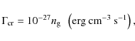
The heating of gas is provided by supernova energy release
as a function of gas temperature Tis calculated from the cooling curves of Wada & Norman (2001) and is linearly interpolated for
metallicities between 10-4 and 1.0 of the solar.
The heating of gas is provided by supernova energy release
![]() ,
cosmic rays
,
cosmic rays
![]() ,
and a background ultraviolet radiation field
,
and a background ultraviolet radiation field
![]() .
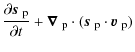
The supernova energy release (per unit time and unit surface area)
is defined as
.
The supernova energy release (per unit time and unit surface area)
is defined as
 |
(11) |
with the lower and upper cutoff masses
 |
(13) |
where
The volume heating and cooling rates in Eq. (10) are assumed to be independent of the z-direction
and are multiplied by the disk thickness (2 Z) to yield the corresponding vertically integrated rates.
The vertical scale height
![]() is calculated via the equation of local pressure balance
in the gravitational field of the dark matter halo, stellar, and gas disks
is calculated via the equation of local pressure balance
in the gravitational field of the dark matter halo, stellar, and gas disks
where
3.3 Instantaneous recycling approximation
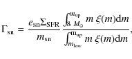
The temporal and spatial evolution of oxygen in our model galaxy is computed adopting
the so-called instantaneous recycling approximation, in which an instantaneous enrichment
by freshly synthesized elements is assumed. This approximation
is valid for the oxygen enrichment, because most of the oxygen
is produced by short-lived, massive stars. We adopt the oxygen yields of
Woosley & Weaver (1995). We assume that oxygen is collisionally coupled to the gas, which eliminates the need
to solve an additional momentum equation for oxygen. The continuity equation for
the oxygen surface density
![]() modified for oxygen production via star formation reads as
modified for oxygen production via star formation reads as
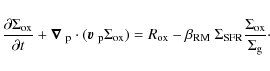
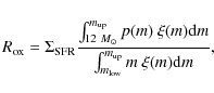
The oxygen production rate per unit area by supernovae is calculated as
 |
(16) |
where p(m) is the mass of oxygen released by a star with mass m (Woosley & Weaver 1995). We assume that the initial oxygen abundance of our model galaxy is
3.4 Code description
An Eulerian finite-difference code is used to solve Eqs. (8)-(10) and (15)
in polar coordinates (![]() ). The basic algorithm of the code is similar
to that of the commonly used ZEUS code. The operator
splitting is utilized to advance in time the dependent variables in two
coordinate directions. The advection is treated using the consistent
transport method and the van Leer interpolation scheme.
There are a few modifications to the usual ZEUS methodology, which are necessitated by the presence
of star formation and cooling and heating processes in our model hydrodynamic equations.
The total hydrodynamic time step
is calculated as a harmonic average of the usual time step due to the Courant-Friedrichs-Lewy condition
and the star formation time step defined as
). The basic algorithm of the code is similar
to that of the commonly used ZEUS code. The operator
splitting is utilized to advance in time the dependent variables in two
coordinate directions. The advection is treated using the consistent
transport method and the van Leer interpolation scheme.
There are a few modifications to the usual ZEUS methodology, which are necessitated by the presence
of star formation and cooling and heating processes in our model hydrodynamic equations.
The total hydrodynamic time step
is calculated as a harmonic average of the usual time step due to the Courant-Friedrichs-Lewy condition
and the star formation time step defined as
![]() .
The internal energy update due to cooling and heating in Eq. (10)
is done implicitly via Newton-Raphson iterations, supplemented by a bisection
algorithm for occasional zones where the Newton-Raphson
method does not converge. This ensures a considerable economy in the CPU time.
A typical run takes about four weeks on four 2.2 GHz Opteron processors.
The resolution is
.
The internal energy update due to cooling and heating in Eq. (10)
is done implicitly via Newton-Raphson iterations, supplemented by a bisection
algorithm for occasional zones where the Newton-Raphson
method does not converge. This ensures a considerable economy in the CPU time.
A typical run takes about four weeks on four 2.2 GHz Opteron processors.
The resolution is
![]() grid zones, which are equidistantly spaced in both
coordinate directions. The radial size of the grid cell is 34 pc and the radial extent of the computational
area is 17 kpc. However, star formation is confined to only the inner 15 kpc.
The code performs well on the angular momentum conservation problem
(see e.g. Vorobyov & Basu 2006). This test problem is essential for the adequate modelling of
rotating systems with radial mass transport.
grid zones, which are equidistantly spaced in both
coordinate directions. The radial size of the grid cell is 34 pc and the radial extent of the computational
area is 17 kpc. However, star formation is confined to only the inner 15 kpc.
The code performs well on the angular momentum conservation problem
(see e.g. Vorobyov & Basu 2006). This test problem is essential for the adequate modelling of
rotating systems with radial mass transport.
3.5 Sporadic star formation
Low gas surface densities (Pickering 1999; de Blok et al. 1996), which are usually below the critical value determined by the Toomre criterion, and low total star formation rates (van den Hoek et al. 2000) argue against large-scale star formation as a viable scenario for LSB galaxies. Despite the low gas surface densities, there is evidence for a noticeable young stellar population as indicated by the blue colors of most LSBs (de Blok et al. 1995). According to de Blok et al. (1995) and Gerretsen & de Blok (1999), a sporadic star formation scenario (i.e. small surges in the SFR, either superimposed on a very low constant SFR or not) can best explain the observed blue colors and evidence for young stars.
There is little known about physical processes that control sporadic star
formation in LSB galaxies. The recent uncalibrated H![]() imaging
of a sample of LSB galaxies by Auld et al. (2006) and the observational data presented here
(see Sect. 4) suggest that star formation is highly clustered.
Current star formation is localized to a handful of
compact regions. There is little or no diffuse H
imaging
of a sample of LSB galaxies by Auld et al. (2006) and the observational data presented here
(see Sect. 4) suggest that star formation is highly clustered.
Current star formation is localized to a handful of
compact regions. There is little or no diffuse H![]() emission coming
from the rest of the galactic disk.
Motivated by this observational evidence, we adopt the sporadic scenario for star formation
in our model LSB galaxy.
emission coming
from the rest of the galactic disk.
Motivated by this observational evidence, we adopt the sporadic scenario for star formation
in our model LSB galaxy.
We use a simple model of sporadic star formation in which the individual star formation
sites (SFSs) are distributed randomly throughout the galactic disk and the star formation
rate per unit area in each SFS is determined by a Schmidt law
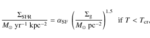
where
 |
(18) |
This means that the adopted star formation efficiency in our model ranges between 0.045 and 0.15 for possible values of the vertical scale height Z=100-1500 pc.
The number of star formation sites at any given time can be roughly determined using the uncalibrated
H![]() images of LSB galaxies by Auld et al. (2006).
These images highlight only a handful of small regions that
have recently formed stars.
There is little diffuse H
images of LSB galaxies by Auld et al. (2006).
These images highlight only a handful of small regions that
have recently formed stars.
There is little diffuse H![]() emission, contrary to the emission in K-, R-, and B-bands
which (as a rule) show a noticeable diffuse component.
The number of HII regions within an individual LSB galaxy identified by van den Hoek et al. (2000) ranges between
4 and 26, with a median number of HII regions equal to 11.
Therefore, the number of SFS,
emission, contrary to the emission in K-, R-, and B-bands
which (as a rule) show a noticeable diffuse component.
The number of HII regions within an individual LSB galaxy identified by van den Hoek et al. (2000) ranges between
4 and 26, with a median number of HII regions equal to 11.
Therefore, the number of SFS,
![]() ,
in our numerical simulations is set to approximately 15.
If we further assume that both
,
in our numerical simulations is set to approximately 15.
If we further assume that both
![]() and the typical area occupied by an individual
star formation site
and the typical area occupied by an individual
star formation site
![]() do not
change significantly with time, this would yield a near-constant mean SFR
over the lifetime of our model galaxy.
However, there is evidence that star formation in blue LSB galaxies
does not proceed at a near-constant rate. Our own numerical simulations and modeling by Zackrisson et al. (2005)
indicate that the SFR should be declining with time to reproduce the
observed H
do not
change significantly with time, this would yield a near-constant mean SFR
over the lifetime of our model galaxy.
However, there is evidence that star formation in blue LSB galaxies
does not proceed at a near-constant rate. Our own numerical simulations and modeling by Zackrisson et al. (2005)
indicate that the SFR should be declining with time to reproduce the
observed H![]() equivalent widths in LSB galaxies. Therefore, we assume that the typical
area occupied by a SFS is a decreasing function of time of the form
equivalent widths in LSB galaxies. Therefore, we assume that the typical
area occupied by a SFS is a decreasing function of time of the form
![]() ,
where
,
where
![]() pc is the area at t=0 and
pc is the area at t=0 and
![]() Gyr
is a characteristic time of exponential decay in the star formation rate.
Gyr
is a characteristic time of exponential decay in the star formation rate.
The duration of star formation in an individual star formation site (
![]() )
is poorly known. We use the theoretical and empirical knowledge
gained by analyzing similar processes in the Solar neighbourhood.
Observations of the current star formation activity in
nearby molecular cloud complexes indicate that the ages of T Tauri stars usually fall in the
1-10 Myr range (Palla & Stahler 2002). Clusters that are 10 Myr old often have little associated
gas remaining, implying that the process shuts off by then. However, the volume gas density
in disks of LSB galaxies is expected to be lower (on average) than that of the Solar neighbourhood,
which may prolong the process of gas conversion into stars. It should also be noted
that individual star formation sites in LSB galaxies have characteristic sizes
that are much larger than those of an individual giant molecular cloud. Otherwise,
we would have to assume unrealistically high star formation efficiency in LSB galaxies
to retrieve the observed star formation rates of the order of
)
is poorly known. We use the theoretical and empirical knowledge
gained by analyzing similar processes in the Solar neighbourhood.
Observations of the current star formation activity in
nearby molecular cloud complexes indicate that the ages of T Tauri stars usually fall in the
1-10 Myr range (Palla & Stahler 2002). Clusters that are 10 Myr old often have little associated
gas remaining, implying that the process shuts off by then. However, the volume gas density
in disks of LSB galaxies is expected to be lower (on average) than that of the Solar neighbourhood,
which may prolong the process of gas conversion into stars. It should also be noted
that individual star formation sites in LSB galaxies have characteristic sizes
that are much larger than those of an individual giant molecular cloud. Otherwise,
we would have to assume unrealistically high star formation efficiency in LSB galaxies
to retrieve the observed star formation rates of the order of
![]() yr-1.
This implies a presence of local triggering mechanisms within an individual SFS
that should also act to prolong the star formation activity.
From the theoretical background, one can argue that the duration of star formation
should be limited by feedback from
newly born massive stars and supernova explosions. The lifetime
of the least massive star capable of producing a supernova is approximately
40 Myr. Hence, the actual lifetime of an individual SFS should lie in between 10 Myr and 40 Myr.
Using spectro-photometric evolution models, van den Hoek et al. (2000) have also found that
yr-1.
This implies a presence of local triggering mechanisms within an individual SFS
that should also act to prolong the star formation activity.
From the theoretical background, one can argue that the duration of star formation
should be limited by feedback from
newly born massive stars and supernova explosions. The lifetime
of the least massive star capable of producing a supernova is approximately
40 Myr. Hence, the actual lifetime of an individual SFS should lie in between 10 Myr and 40 Myr.
Using spectro-photometric evolution models, van den Hoek et al. (2000) have also found that
![]() Myr
reproduce well the observed (R-I) colors and I-band luminosities of LSB galaxies.
In our numerical simulations we assume that
Myr
reproduce well the observed (R-I) colors and I-band luminosities of LSB galaxies.
In our numerical simulations we assume that
![]() Myr. Thus, each twenty
million years we initialize a new set of SFSs (
Myr. Thus, each twenty
million years we initialize a new set of SFSs (
![]() )
and randomly distribute them in the inner 15 kpc of the galactic disk.
Each SFS is assigned a velocity equal to that of the local gas velocity upon
its creation and is evolved collisionlessly in the total gravitational
potential of the stellar disk and the dark matter halo using the
fifth-order Runge-Kutta Cash-Karp integration scheme. The old SFSs are rendered inactive
and their further evolution is not computed.
)
and randomly distribute them in the inner 15 kpc of the galactic disk.
Each SFS is assigned a velocity equal to that of the local gas velocity upon
its creation and is evolved collisionlessly in the total gravitational
potential of the stellar disk and the dark matter halo using the
fifth-order Runge-Kutta Cash-Karp integration scheme. The old SFSs are rendered inactive
and their further evolution is not computed.
4 Observations
There is only a small number of (nearby) LSB galaxies
with published H![]() images, which would allow the study
of the distribution and properties of their star-formation regions.
H
images, which would allow the study
of the distribution and properties of their star-formation regions.
H![]() images of about 18 LSB galaxies are available in
McGaugh et al. (1995b); McGaugh & Bothun (1994),
while de Blok & van der Hulst (1998) only published the spectra and
some broad band images. A new sample of 6 LSB galaxies was
presented in Auld et al. (2006).
images of about 18 LSB galaxies are available in
McGaugh et al. (1995b); McGaugh & Bothun (1994),
while de Blok & van der Hulst (1998) only published the spectra and
some broad band images. A new sample of 6 LSB galaxies was
presented in Auld et al. (2006).
From the image data set (McGaugh, priv. comm.)
we selected 4 LSB spiral galaxies based on their B band morphology.
We selected the galaxies to be close to face-on and showing different
disk surface brightness and spiral morphology. This resulted in
UGC 9024, UGC 12845, UGC 5675, and UGC 6151.
A different version of the H![]() images of UGC 9024, UGC 5675,
and UGC 6151 was previously published in McGaugh et al. (1995b).
images of UGC 9024, UGC 5675,
and UGC 6151 was previously published in McGaugh et al. (1995b).
For in Fig. 3 we improved the cosmic rays
rejection and correction of detection blemishes of the
already flat-fielded images. The generation of the continuum corrected
H![]() images followed closely the schema described
e.g. in Bomans (1997).
We realigned the H
images followed closely the schema described
e.g. in Bomans (1997).
We realigned the H![]() and continuum
images carefully using the foreground stars visible in
both images to sub-pixel accuracy and subtracted the scaled
continuum image. We tested different scaling factors and
defined an optimal subtraction based on the disappearance of the
stellar disk of the LSB galaxy. These factors also gave the
smallest foreground star residuals and is consistent with
the scaling factor calculated by measuring the flux of several
foreground stars in both images.
and continuum
images carefully using the foreground stars visible in
both images to sub-pixel accuracy and subtracted the scaled
continuum image. We tested different scaling factors and
defined an optimal subtraction based on the disappearance of the
stellar disk of the LSB galaxy. These factors also gave the
smallest foreground star residuals and is consistent with
the scaling factor calculated by measuring the flux of several
foreground stars in both images.
![\begin{figure}
\par\includegraphics[angle=-90,width=9cm,clip]{10320fg3.eps}
\end{figure}](/articles/aa/full_html/2009/38/aa10320-08/img142.png) |
Figure 3: Reprocessed and continuum subtracted images of the LSB galaxies UGC 9024 ( upper left), UGC 12845 ( upper right), UGC 5675 ( lower left), and UGC 6151 ( lower right). |
| Open with DEXTER | |
The distribution of the HII regions in all 4 galaxies in Fig. 3
is consistent with the predicted pattern of sporadic star formation.
The H![]() images of 6 LSB galaxies recently published by
Auld et al. (2006) show the same behavior, as do the other
galaxies published in McGaugh et al. (1995b).
images of 6 LSB galaxies recently published by
Auld et al. (2006) show the same behavior, as do the other
galaxies published in McGaugh et al. (1995b).
5 Numerical results
5.1 Gas density and temperature distribution
The model galaxy described in Sect. 3 will be
referred hereafter as model 1. We will also introduce other
models that have identical structural properties such as those summarized in Table 1
but different IMFs and star formation rates.
We start our numerical simulations by setting the equilibrium gas disk and slowly introducing
the non-axisymmetric gravitational potential of the stellar spiral arms. Specifically,
![]() is multiplied by
a function
is multiplied by
a function ![]() ,
which has a value of 0 at t=0 and linearly
grows to its maximum value of 1.0 at
,
which has a value of 0 at t=0 and linearly
grows to its maximum value of 1.0 at ![]() Myr.
It takes another hundred million years for the gas disk to adjust to the spiral gravitational potential
and develop a spiral structure. Figure 4 shows the gas
surface density distribution (in log units) in the 1 Gyr old (upper left),
2 Gyr old (upper right), 5 Gyr old, (lower left), and 12 Gyr old (lower right) disks.
It is seen that the gas disk develops a strong phase separation with age.
While the initial gas disk has surface densities between
Myr.
It takes another hundred million years for the gas disk to adjust to the spiral gravitational potential
and develop a spiral structure. Figure 4 shows the gas
surface density distribution (in log units) in the 1 Gyr old (upper left),
2 Gyr old (upper right), 5 Gyr old, (lower left), and 12 Gyr old (lower right) disks.
It is seen that the gas disk develops a strong phase separation with age.
While the initial gas disk has surface densities between
![]() pc-2 and
pc-2 and
![]() pc-2,
the 1-Gyr-old disk features some dense clumps with surface densities in excess of
pc-2,
the 1-Gyr-old disk features some dense clumps with surface densities in excess of
![]() pc-2and temperatures of 100-200 K. The number of such clumps increases with time and they are
stretched
into extended filaments and arcs by galactic differential rotation. Observational detection
of such features could be a powerful test on the sporadic nature of star formation in LSB galaxies.
The gas response to the underlying spiral stellar density wave is rather weak in the early
disk evolution and can hardly be noticed in the 5 and 13 Gyr old disks. This implies that mixing
due to spiral stellar density waves is inefficient in the old disk.
pc-2and temperatures of 100-200 K. The number of such clumps increases with time and they are
stretched
into extended filaments and arcs by galactic differential rotation. Observational detection
of such features could be a powerful test on the sporadic nature of star formation in LSB galaxies.
The gas response to the underlying spiral stellar density wave is rather weak in the early
disk evolution and can hardly be noticed in the 5 and 13 Gyr old disks. This implies that mixing
due to spiral stellar density waves is inefficient in the old disk.
![\begin{figure}
\par\includegraphics[width=9cm,clip]{10320fg4.eps}
\end{figure}](/articles/aa/full_html/2009/38/aa10320-08/img148.png) |
Figure 4:
Gas surface density distribution in the 1-Gyr-old ( upper left), 2-Gyr-old ( upper right), 5-Gyr-old ( lower left), and 12-Gyr-old ( lower right) disks. Dark regions are the densest and coldest. The scale bar is |
| Open with DEXTER | |
![\begin{figure}
\par\includegraphics[width=9cm,clip]{10320fg5.eps}
\end{figure}](/articles/aa/full_html/2009/38/aa10320-08/img149.png) |
Figure 5: Gas mass per Kelvin versus temperature in disks of distinct age as indicated in the legend. The two peaks manifest the phase separation. Note that there is little gas with a temperature below 40 K. |
| Open with DEXTER | |
The phase separation of the gas disk can be illustrated
by calculating the gas mass per unit temperature band at different evolutionary times.
Figure 5 shows the gas mass per Kelvin as a function of temperature at t=2 Gyr (solid line),
t=5 Gyr (dashed line) and t=13 Gyr (dash-dotted line). There are two prominent peaks that
manifest the separation of the gas into two phases - a cold gas phase with a peak temperature of
T=50-100 K and a warm gas phase with a peak temperature of
![]() K.
The positions of the peaks drift apart as the gas disk evolves, indicating that the cold phase becomes
colder and the warm phase becomes warmer with time. However, the gas temperature never drops below 35 K.
It is also evident from the amplitudes of the peaks that the cold phase accumulates
gas mass with time, which is explained by increased cooling due to ongoing heavy element
production. A similar phase separation was also obtained in numerical simulations of LSBs by Gerretsen & de Blok (1999).
The fact that there is little gas with temperature below 35 K implies
that most of the cold phase may be in the form of atomic rather than molecular hydrogen,
but more accurate numerical simulations with a chemical reaction network and higher
numerical resolution are needed to prove this hypothesis.
K.
The positions of the peaks drift apart as the gas disk evolves, indicating that the cold phase becomes
colder and the warm phase becomes warmer with time. However, the gas temperature never drops below 35 K.
It is also evident from the amplitudes of the peaks that the cold phase accumulates
gas mass with time, which is explained by increased cooling due to ongoing heavy element
production. A similar phase separation was also obtained in numerical simulations of LSBs by Gerretsen & de Blok (1999).
The fact that there is little gas with temperature below 35 K implies
that most of the cold phase may be in the form of atomic rather than molecular hydrogen,
but more accurate numerical simulations with a chemical reaction network and higher
numerical resolution are needed to prove this hypothesis.
![\begin{figure}
\par\includegraphics[width=9cm,clip]{10320fg6.eps}
\end{figure}](/articles/aa/full_html/2009/38/aa10320-08/img151.png) |
Figure 6: Star formation rate versus time in model 1. The solid and thick dashed lines show the SFR averaged over 20 Myr and 1.0 Gyr, respectively. Note large amplitude fluctuations in the 20 Myr averaged SFRs around the 1 Gyr averaged values. |
| Open with DEXTER | |
Figure 5 indicates that model 1 has no hot gas phase with temperatures of
order 106 K, which is a consequence of a relatively low SFR and moderate numerical resolution.
The energy injection by star formation of such a low rate
is not enough to convert all gas in a computational cell (
![]() pc) to
the hot phase. This is because we solve the equations of hydrodynamics for a single fluid.
As a consequence, the temperature of all gas
in a computational cell is characterized by a specific value and
there is no gas
phase separation within an individual cell. This, however, does not mean that the hot gas
is not present at all
in LSB galaxies, we simply may need a much higher numerical resolution to resolve it.
We do start seeing the hot phase if we increase the SFR in our model by a factor of several.
We note that Gerretsen & de Blok (1999)
have also found little hot gas in their numerical simulations.
pc) to
the hot phase. This is because we solve the equations of hydrodynamics for a single fluid.
As a consequence, the temperature of all gas
in a computational cell is characterized by a specific value and
there is no gas
phase separation within an individual cell. This, however, does not mean that the hot gas
is not present at all
in LSB galaxies, we simply may need a much higher numerical resolution to resolve it.
We do start seeing the hot phase if we increase the SFR in our model by a factor of several.
We note that Gerretsen & de Blok (1999)
have also found little hot gas in their numerical simulations.
Figure 6 shows the SFR as a function of time in model 1.
In particular, the solid line presents the SFR averaged over the past 20 Myr; these values
are later used to construct H![]() equivalent widths.
In addition, the thick dashed line plots the SFR averaged over a 1 Gyr interval centered
on the current time (running average method).
It is seen that the 20 Myr averaged SFRs have considerable fluctuations around
the 1 Gyr averaged values.
These fluctuations have a characteristic time scale of a few hundred Myr and
amplitudes that may exceed
equivalent widths.
In addition, the thick dashed line plots the SFR averaged over a 1 Gyr interval centered
on the current time (running average method).
It is seen that the 20 Myr averaged SFRs have considerable fluctuations around
the 1 Gyr averaged values.
These fluctuations have a characteristic time scale of a few hundred Myr and
amplitudes that may exceed
![]() yr-1.
The existence of such bursts of star formation is an essential ingredient for successful modelling
of blue colors of at least some LSB galaxies (e.g. van den Hoek et al. 2000). Similar fluctuations in the SFR
were also observed in numerical simulations by Gerretsen & de Blok (1999).
The 1 Gyr averaged SFR quickly grows to a maximum value
yr-1.
The existence of such bursts of star formation is an essential ingredient for successful modelling
of blue colors of at least some LSB galaxies (e.g. van den Hoek et al. 2000). Similar fluctuations in the SFR
were also observed in numerical simulations by Gerretsen & de Blok (1999).
The 1 Gyr averaged SFR quickly grows to a maximum value
![]() yr-1
at t=2.6 Gyr and subsequently declines to
yr-1
at t=2.6 Gyr and subsequently declines to
![]() yr-1 at t=13.0 Gyr.
Typical star formation rates in LSB galaxies range
from 0.02 to
yr-1 at t=13.0 Gyr.
Typical star formation rates in LSB galaxies range
from 0.02 to
![]() yr-1, with a median SFR of
yr-1, with a median SFR of
![]() yr-1 (van den Hoek et al. 2000).
Model 1 yields SFRs that are consistent with the inferred present-day rates.
yr-1 (van den Hoek et al. 2000).
Model 1 yields SFRs that are consistent with the inferred present-day rates.
5.2 Radial variations in the oxygen abundance
We calculate the oxygen abundance
![]() in our disk from the model's known surface densities of gas
(
in our disk from the model's known surface densities of gas
(
![]() )
and oxygen (
)
and oxygen (
![]() ).
We find that the spatial distribution of oxygen in the 1 Gyr old
gas disk has a pronounced patchy appearance - local regions with enhanced oxygen abundance
adjoin local regions with low oxygen abundance. The local contrast in [O/H] may be as
large as 1.0 dex or even more. As the galaxy evolves, the spatial
distribution of oxygen becomes noticeably smoother. The smearing is caused by stirring
due to differential rotation, radial migration of gas triggered
by the non-axisymmetric gravitational potential of stellar spiral arms, and energy release
of supernova explosions.
).
We find that the spatial distribution of oxygen in the 1 Gyr old
gas disk has a pronounced patchy appearance - local regions with enhanced oxygen abundance
adjoin local regions with low oxygen abundance. The local contrast in [O/H] may be as
large as 1.0 dex or even more. As the galaxy evolves, the spatial
distribution of oxygen becomes noticeably smoother. The smearing is caused by stirring
due to differential rotation, radial migration of gas triggered
by the non-axisymmetric gravitational potential of stellar spiral arms, and energy release
of supernova explosions.
To better illustrate the spatial variations in the oxygen distribution in model 1,
we show in Fig. 7 the radial profiles of the oxygen abundance
obtained by making a narrow (![]() 50 pc) radial cut through the galactic disk at
50 pc) radial cut through the galactic disk at
![]() .
The numbers in each frame indicate the age of our model galaxy. The most prominent
feature in Fig. 7 is a sharp decline in the typical amplitude of the radial fluctuations
in [O/H]. For instance, the radial distribution of the oxygen abundance
in the 1 Gyr old disk is very irregular and shows radial fluctuations with amplitudes as large
as 1.0 dex and even more. The fluctuations have a short characteristic radial scale of
the order of 1-2 kpc. The fluctuation amplitudes have noticeably decreased in the 2 Gyr old disk,
which now has a maximum amplitude of the order of 0.5 dex.
The 5 Gyr old disk (and older disks) feature only low-amplitude fluctuations
in the oxygen abundance with amplitudes rarely exceeding 0.2 dex.
.
The numbers in each frame indicate the age of our model galaxy. The most prominent
feature in Fig. 7 is a sharp decline in the typical amplitude of the radial fluctuations
in [O/H]. For instance, the radial distribution of the oxygen abundance
in the 1 Gyr old disk is very irregular and shows radial fluctuations with amplitudes as large
as 1.0 dex and even more. The fluctuations have a short characteristic radial scale of
the order of 1-2 kpc. The fluctuation amplitudes have noticeably decreased in the 2 Gyr old disk,
which now has a maximum amplitude of the order of 0.5 dex.
The 5 Gyr old disk (and older disks) feature only low-amplitude fluctuations
in the oxygen abundance with amplitudes rarely exceeding 0.2 dex.
![\begin{figure}
\par\includegraphics[width=9cm,clip]{10320fg7.eps}
\end{figure}](/articles/aa/full_html/2009/38/aa10320-08/img158.png) |
Figure 7:
Radial profiles of [O/H] obtained by making a narrow cut through the galactic disk at an azimuthal angle
|
| Open with DEXTER | |
![\begin{figure}
\par\includegraphics[width=9cm,clip]{10320fg8.eps}
\end{figure}](/articles/aa/full_html/2009/38/aa10320-08/img159.png) |
Figure 8: Oxygen abundance fluctuation spectrum defined as the normalized number of radial oxygen abundance fluctuations versus fluctuation amplitude (in dex). Lines of distinct color correspond to different numerical models and lines of distinct type correspond to different galactic ages as indicated. See the text for more details. |
| Open with DEXTER | |
Figure 7 reveals the absence of any significant radial abundance gradients in our model disk. This appears to be typical of LSB galaxies (e.g. de Blok & van der Hulst 1998). The lack of radial abundance gradients is most likely caused by a spatially and temporally sporadic nature of star formation, i.e., LSB galaxies must have evolved at the same rate over their entire disk. Well-known star formation threshold criteria, such as those based on the gas surface density threshold (Toomre criterion) or the rate of shear (Vorobyov 2003; Martin & Kennicutt 2001), would increase the likelihood of star formation in regions of higher density and lower angular velocity, which are usually the inner galactic regions. As a result, negative radial abundance gradients may develop with time. The fact that we do not see radial abundance gradients in LSB galaxies implies that star formation has no threshold barrier.
Table 2: Summary of galactic models.
To analyze the properties of the oxygen abundance fluctuations
in disks of different age, we calculate the fluctuation spectrum defined as
the (normalized) number of fluctuations versus the fluctuation amplitude A.
The latter is
calculated in the following manner. We scan the disk in the radial
direction along each azimuthal angle (![]() )
of our numerical polar grid
for the adjacent minima and maxima in the oxygen abundance distribution.
The absolute value of the difference between the adjacent minimum and maximum (or vice versa)
gives us the radial amplitude of a fluctuation on spatial scales of our numerical resolution,
)
of our numerical polar grid
for the adjacent minima and maxima in the oxygen abundance distribution.
The absolute value of the difference between the adjacent minimum and maximum (or vice versa)
gives us the radial amplitude of a fluctuation on spatial scales of our numerical resolution,
![]() 40 pc. The calculated fluctuation amplitudes are distributed in 40 logarithmically spaced
bins between 0.1 dex and 3.0 dex and then normalized by the total number
of fluctuations in all bins. The resulting fluctuation spectrum has the meaning
of the probability function
40 pc. The calculated fluctuation amplitudes are distributed in 40 logarithmically spaced
bins between 0.1 dex and 3.0 dex and then normalized by the total number
of fluctuations in all bins. The resulting fluctuation spectrum has the meaning
of the probability function
![]() - the product of the total number of fluctuations and
- the product of the total number of fluctuations and
![]() yields the number of fluctuation with amplitude A.
yields the number of fluctuation with amplitude A.
Figure 8 shows the probability function
![]() derived for four models detailed below. Hereafter, different
line types in Fig. 8 will help to distinguish between galaxies of distinct age
and different line colors will correspond to different numerical models.
Black lines present
derived for four models detailed below. Hereafter, different
line types in Fig. 8 will help to distinguish between galaxies of distinct age
and different line colors will correspond to different numerical models.
Black lines present
![]() in model 1 for the 1 Gyr old disk (solid line),
2 Gyr old disk (dashed line), 5 Gyr old disk (dash-dotted line),
and 12 Gyr old disk (dash-dot-dotted line). It is evident that the probability functions for disks of
different ages intermix for
in model 1 for the 1 Gyr old disk (solid line),
2 Gyr old disk (dashed line), 5 Gyr old disk (dash-dotted line),
and 12 Gyr old disk (dash-dot-dotted line). It is evident that the probability functions for disks of
different ages intermix for
![]() but appear to be quite distinct
for
but appear to be quite distinct
for
![]() .
Can this peculiar feature of
.
Can this peculiar feature of
![]() be used to constrain the age of LSB galaxies? The extent to which oxygen is spatially mixed
in the galactic disk may depend on the model parameters such as the strength of the
spiral density wave, shape of the IMF, and details of the energy release by SNe.
In order to estimate the dependence of
be used to constrain the age of LSB galaxies? The extent to which oxygen is spatially mixed
in the galactic disk may depend on the model parameters such as the strength of the
spiral density wave, shape of the IMF, and details of the energy release by SNe.
In order to estimate the dependence of
![]() on these factors, we run two test models. Model T1 has no spiral density waves and
model T2 is characterized by a factor of 2 lower energy input by SNe (``T'' stands for ``test''
to distinguish them from regular models).
Model T2 attempts
to mimic the case when part of the SN energy is lost to the extragalactic medium via SN bubbles.
It is also important to see the effect that a different IMF may have on the probability function.
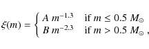
Therefore, we introduced model 2, which is characterized by the Salpeter IMF with
the upper and lower cut-off masses of
on these factors, we run two test models. Model T1 has no spiral density waves and
model T2 is characterized by a factor of 2 lower energy input by SNe (``T'' stands for ``test''
to distinguish them from regular models).
Model T2 attempts
to mimic the case when part of the SN energy is lost to the extragalactic medium via SN bubbles.
It is also important to see the effect that a different IMF may have on the probability function.
Therefore, we introduced model 2, which is characterized by the Salpeter IMF with
the upper and lower cut-off masses of
![]() and
and
![]() .
Model 2
has the same structural parameters as model 1 except for
.
Model 2
has the same structural parameters as model 1 except for
![]() which is set to 18.5 Gyr.
The parameters of models 1 and 2 are detailed in Table 2.
The probability functions corresponding
to model T1, model T2, and model 2 are shown in the top panel of Fig. 8
by the red, blue, and cyan lines, respectively. The meaning of the line types
(i.e., solid, dashed, etc.) is indicated in the figure.
which is set to 18.5 Gyr.
The parameters of models 1 and 2 are detailed in Table 2.
The probability functions corresponding
to model T1, model T2, and model 2 are shown in the top panel of Fig. 8
by the red, blue, and cyan lines, respectively. The meaning of the line types
(i.e., solid, dashed, etc.) is indicated in the figure.
A noticeable scatter in the probability
functions of distinct age is seen
among different models. In particular, the probability functions of galaxies of 5-12 Gyr age
intermingle and thus cannot be used to make age predictions. However, it is still possible
to differentiate between (1-2) Gyr old and (5-12) Gyr old galaxies based
on the slope of
![]() .
Young galaxies of 1-2 Gyr age have fluctuation spectra with
a much shallower slope than (5-13) Gyr old galaxies, meaning that the former
feature radial oxygen abundance fluctuations of much larger amplitude than the latter.
A similar behaviour of
.
Young galaxies of 1-2 Gyr age have fluctuation spectra with
a much shallower slope than (5-13) Gyr old galaxies, meaning that the former
feature radial oxygen abundance fluctuations of much larger amplitude than the latter.
A similar behaviour of
![]() is found
when we decrease the spatial resolution of the fluctuation amplitude measurements
from 40 pc to several hundred parsecs (more appropriate for modern observational techniques).
We conclude that measurements of the radial oxygen abundance fluctuations may be used only to
set order-of-magnitude constraints on the age of blue LSB galaxies.
is found
when we decrease the spatial resolution of the fluctuation amplitude measurements
from 40 pc to several hundred parsecs (more appropriate for modern observational techniques).
We conclude that measurements of the radial oxygen abundance fluctuations may be used only to
set order-of-magnitude constraints on the age of blue LSB galaxies.
We are aware of only one successful measurement of the radial abundance
gradients in three LSB galaxies done by de Blok & van der Hulst (1998). Unfortunately, the number
of resolved HII regions and oxygen abundance measurements in each galaxy is too low (<10)
to make a meaningful comparison with our predictions.
With such a small sample, the probability function would be confined in the
![]() range,
which is not helpful for making age predictions due to degeneracy of
range,
which is not helpful for making age predictions due to degeneracy of
![]() in this range.
in this range.
6 Constraining the age of blue LSB galaxies
In this section, we investigate if the time evolution of the
mean oxygen abundance,
complemented by H![]() emission equivalent widths
and optical colors, can be used to better constrain the age of blue LSB galaxies.
We consider several new models (in addition to our models 1 and 2) that have different
rates of star formation.
emission equivalent widths
and optical colors, can be used to better constrain the age of blue LSB galaxies.
We consider several new models (in addition to our models 1 and 2) that have different
rates of star formation.
6.1 Time evolution of the oxygen abundance
There have been several efforts in the past to measure the oxygen abundances in HII
regions of blue LSB galaxies. For instance, oxygen abundances in a sample of 18
galaxies in Kuzio de Narray et al. (2004) have a median value
![]() .
Their smallest and largest measured abundances (using the equivalent width method)
are
.
Their smallest and largest measured abundances (using the equivalent width method)
are
![]() (F611-1) and
(F611-1) and
![]() (UGC 5709).
de Blok & van der Hulst (1998) have observed 64 HII regions in 12 LSB galaxies and derived oxygen abundances
that peak around
(UGC 5709).
de Blok & van der Hulst (1998) have observed 64 HII regions in 12 LSB galaxies and derived oxygen abundances
that peak around
![]() .
The lowest abundance in their sample is
.
The lowest abundance in their sample is
![]() .
These data demonstrate that the present day mean oxygen abundance in LSB galaxies is about
.
These data demonstrate that the present day mean oxygen abundance in LSB galaxies is about
![]() dex, albeit with a wide scatter.
We plot the minimum and maximum oxygen abundances found in blue LSB galaxies by horizontal dotted
lines in Fig. 9, while the mean oxygen abundance
for LSB galaxies is shown by the vertical dash-dot-dotted line.
dex, albeit with a wide scatter.
We plot the minimum and maximum oxygen abundances found in blue LSB galaxies by horizontal dotted
lines in Fig. 9, while the mean oxygen abundance
for LSB galaxies is shown by the vertical dash-dot-dotted line.
The amount of produced oxygen and the oxygen abundance are expected to depend on the adopted rate of star formation and on the details of the initial mass function. Most of oxygen is produced by intermediate to massive stars and both the slope and the upper mass cutoff are those parameters of the IMF that may influence the rate of oxygen production. In this paper, we study IMFs of different slope, leaving cut-off IMFs for a subsequent study.
![\begin{figure}
\par\includegraphics[width=9cm,clip]{10320fg9.eps}
\end{figure}](/articles/aa/full_html/2009/38/aa10320-08/img175.png) |
Figure 9: Mean oxygen abundance as a function of galactic age. Each line type corresponds to a particular numerical model as indicated in the figure. The horizontal dotted lines delineate the range of oxygen abundances found in blue LSB galaxies (de Blok & van der Hulst 1998; Kuzio de Narray et al. 2004) and the horizontal dashed-dot-dotted line shows the mean oxygen abundance derived from a large sample of LSB galaxies. See the text and Table 2 for more details. |
| Open with DEXTER | |
The mean oxygen abundances
![]() obtained in
model 1 are presented in Fig. 9 by the thick solid line. The mean values are
calculated by summing up local oxygen abundances in each computational cell
between 1 kpc and 14 kpc and then averaging over the corresponding number of cells.
The dashed line shows
obtained in
model 1 are presented in Fig. 9 by the thick solid line. The mean values are
calculated by summing up local oxygen abundances in each computational cell
between 1 kpc and 14 kpc and then averaging over the corresponding number of cells.
The dashed line shows
![]() as a function
of galactic age in model 2. In addition, we have introduced two more models that have structural
parameters identical to those of models 1 and 2 (see Table 1) but are characterized
by lower SFRs. In particular, models 1L and 2L (thin solid line/dash-dotted line) feature on
average a factor of 1.4 lower rates of star formation than models 1 and 2.
The parameters of models 1L and 2L, as well as the minimum and maximum SFRs,
are listed in Table 2. It is evident that models with the Salpeter IMF yield
lower
as a function
of galactic age in model 2. In addition, we have introduced two more models that have structural
parameters identical to those of models 1 and 2 (see Table 1) but are characterized
by lower SFRs. In particular, models 1L and 2L (thin solid line/dash-dotted line) feature on
average a factor of 1.4 lower rates of star formation than models 1 and 2.
The parameters of models 1L and 2L, as well as the minimum and maximum SFRs,
are listed in Table 2. It is evident that models with the Salpeter IMF yield
lower
![]() than the corresponding models with the Kroupa IMF.
With the lower and upper mass limits being identical, the Sapleter IMF may
be regarded bottom-heavy
in comparison to that of Kroupa. A bottom-heavy IMF has a lower relative number of massive stars
and this fact accounts for the lower rate of oxygen production in models with the Salpeter IMF.
Furthermore, models with lower SFRs yield lower mean oxygen abundances.
than the corresponding models with the Kroupa IMF.
With the lower and upper mass limits being identical, the Sapleter IMF may
be regarded bottom-heavy
in comparison to that of Kroupa. A bottom-heavy IMF has a lower relative number of massive stars
and this fact accounts for the lower rate of oxygen production in models with the Salpeter IMF.
Furthermore, models with lower SFRs yield lower mean oxygen abundances.
There are several interesting conclusions that can be drawn by analyzing
Fig. 9. First, our models can reproduce the entire range of observed oxygen abundances
found in LSB galaxies (delimited by horizontal dotted lines).
Second, for a given value of
![]() ,
the predicted ages show a large scatter
(that increases along the sequence of increasing oxygen abundances),
making mean oxygen abundances alone a poor age indicator, especially for metal-rich LSBs.
Finally, the minimum oxygen abundance found among LSB galaxies
(bottom dotted line in Fig. 9) can be attained after just
1-3.5 Gyr of evolution, suggesting a possibility of rather young age
for LSB galaxies. We will return to this issue in some more detail
in the following section.
,
the predicted ages show a large scatter
(that increases along the sequence of increasing oxygen abundances),
making mean oxygen abundances alone a poor age indicator, especially for metal-rich LSBs.
Finally, the minimum oxygen abundance found among LSB galaxies
(bottom dotted line in Fig. 9) can be attained after just
1-3.5 Gyr of evolution, suggesting a possibility of rather young age
for LSB galaxies. We will return to this issue in some more detail
in the following section.
6.2 H equivalent widths and B-V integrated colors
In this section we use population synthesis modelling to
calculate the integrated B-V colors and H![]() equivalent widths (EW(H
equivalent widths (EW(H![]() )) using the model's
known SFRs and mean oxygen abundances. The interested reader can find details of the population
synthesis model and essential tests in the Appendix.
There is observational evidence that LSB galaxies are characterized by B-V colors and EW(H
)) using the model's
known SFRs and mean oxygen abundances. The interested reader can find details of the population
synthesis model and essential tests in the Appendix.
There is observational evidence that LSB galaxies are characterized by B-V colors and EW(H![]() )
that lie in certain limits. For instance, the observed B-V colors of blue LSB galaxies
(which we attempt to model in this paper) appear to lie in the 0.3-0.7 range (de Blok et al. 1995).
According to Zackrisson et al. (2005), EW(H
)
that lie in certain limits. For instance, the observed B-V colors of blue LSB galaxies
(which we attempt to model in this paper) appear to lie in the 0.3-0.7 range (de Blok et al. 1995).
According to Zackrisson et al. (2005), EW(H![]() )
of a sample of blue LSB galaxies seem to be confined
within rather narrow bounds,
)
of a sample of blue LSB galaxies seem to be confined
within rather narrow bounds,
![]() Å. Hence, population synthesis modelling
may be regarded as a consistency test for our numerical models, which should yield
EW(H
Å. Hence, population synthesis modelling
may be regarded as a consistency test for our numerical models, which should yield
EW(H![]() )
and B-V colors in acceptable agreement with observations.
)
and B-V colors in acceptable agreement with observations.
We present the results of population synthesis modelling only for models with different
IMFs; models with different SFRs show a similar behaviour. Figure 10
shows model EW(H![]() (left column) and B-Vcolors (right column) as a function of galactic age for model 1 (top)
and model 2 (bottom). The equivalent widths are derived using SFRs averaged over the past 20 Myr.
For convenience, the thick dashed lines show EW(H
(left column) and B-Vcolors (right column) as a function of galactic age for model 1 (top)
and model 2 (bottom). The equivalent widths are derived using SFRs averaged over the past 20 Myr.
For convenience, the thick dashed lines show EW(H![]() )
averaged over 1 Gyr.
The horizontal dotted lines in the left
panels show a typical range for EW(H
)
averaged over 1 Gyr.
The horizontal dotted lines in the left
panels show a typical range for EW(H![]() )
in blue LSB galaxies (Zackrisson et al. 2005),
while the horizontal dotted lines in the right panels outline typical B-V colors of blue
LSB galaxies (de Blok et al. 1995). The arrow shows a (possible) reddening due to dust extinction
for a fiducial value of the color excess
E(B-V)=0.1 (McGaugh 1994).
)
in blue LSB galaxies (Zackrisson et al. 2005),
while the horizontal dotted lines in the right panels outline typical B-V colors of blue
LSB galaxies (de Blok et al. 1995). The arrow shows a (possible) reddening due to dust extinction
for a fiducial value of the color excess
E(B-V)=0.1 (McGaugh 1994).
![\begin{figure}
\par\includegraphics[width=9cm,clip]{10320fg10.eps}
\end{figure}](/articles/aa/full_html/2009/38/aa10320-08/img179.png) |
Figure 10:
H |
| Open with DEXTER | |
It is evident that model EW(H![]() )
show considerable
fluctuations of the order of 15-20 Å around mean values, which reflect the corresponding
fluctuations in the SFR. Neither model 1 nor model 2 can account for the observed equivalent widths
in the early evolution, yielding too large EW(H
)
show considerable
fluctuations of the order of 15-20 Å around mean values, which reflect the corresponding
fluctuations in the SFR. Neither model 1 nor model 2 can account for the observed equivalent widths
in the early evolution, yielding too large EW(H![]() )
during the first 5-6 Gyr.
Both models begin to match the observed EW(H
)
during the first 5-6 Gyr.
Both models begin to match the observed EW(H![]() )
only in the late evolution after 6 Gyr,
with model 2 (Salpeter IMF) yielding a somewhat better fit.
We note that all models feature short-term variations in EW(H
)
only in the late evolution after 6 Gyr,
with model 2 (Salpeter IMF) yielding a somewhat better fit.
We note that all models feature short-term variations in EW(H![]() )
of such an amplitude that the corresponding equivalent widths may accidently go beyond either the
upper or lower observed limits in the late evolution phase.
This is however not alarming, since these fluctuations are short-lived and the
observed range is inferred from
just a few galaxies and may increase as more observational data become available.
)
of such an amplitude that the corresponding equivalent widths may accidently go beyond either the
upper or lower observed limits in the late evolution phase.
This is however not alarming, since these fluctuations are short-lived and the
observed range is inferred from
just a few galaxies and may increase as more observational data become available.
Unlike model EW(H![]() ), there are no large short-term fluctuations
in model B-V colors shown in the right column of Fig. 10.
Younger galaxies have on average bluer colors. The lowest observed color B-V=0.3
is reached after approximately 2.5-3.0 Gyr of evolution.
Taking into account a possible reddening, the latter value may decrease to approximately
1.5-2.0 Gyr. A similar lower limit on the galactic age was inferred from
numerical modelling of oxygen abundances in Sect. 6.1.
However, model equivalent widths suggest a much larger value,
), there are no large short-term fluctuations
in model B-V colors shown in the right column of Fig. 10.
Younger galaxies have on average bluer colors. The lowest observed color B-V=0.3
is reached after approximately 2.5-3.0 Gyr of evolution.
Taking into account a possible reddening, the latter value may decrease to approximately
1.5-2.0 Gyr. A similar lower limit on the galactic age was inferred from
numerical modelling of oxygen abundances in Sect. 6.1.
However, model equivalent widths suggest a much larger value, ![]() 5-6 Gyr.
This value may decrease slightly, if LSB galaxies feature truncated IMFs with a smaller
upper mass limit, say 40
5-6 Gyr.
This value may decrease slightly, if LSB galaxies feature truncated IMFs with a smaller
upper mass limit, say 40 ![]() instead of 100
instead of 100 ![]() .
The oxygen abundance fluctuation spectrum
.
The oxygen abundance fluctuation spectrum
![]() can be used to better constrain the minimum
age of blue LSB galaxies.
can be used to better constrain the minimum
age of blue LSB galaxies.
It is well known that blue LSB galaxies have B-V colors that are systematically bluer than those of HSB galaxies (de Blok et al. 1995). It is tempting to assume that this fact may be indicative of blue LSB galaxies being systematically younger than their HSB counterparts. However, our evolved galaxies seem to have colors that fall within the observed limits. There is a slight possibility that the model B-V color will exceed the upper observed limit if dust extinction is taken into account. But considering the uncertainty in dust content in blue LSB galaxies, this possibility is not conclusive. Even if blue LSB galaxies are younger than their HSB counterparts, the difference in age is not dramatic, of the order of a few Gyr at most. It is likely that blue LSB galaxies owe their bluer than usual colors to the sporadic nature of star formation (see e.g. de Blok et al. 1995; Gerretsen & de Blok 1999; McGaugh 1994).
6.3 Mean oxygen abundances versus H
equivalent widths
Finally, we present the
![]() diagram in Fig. 11. Each symbol in this diagram
represents a pair of data points
diagram in Fig. 11. Each symbol in this diagram
represents a pair of data points
![]() corresponding to a specific galactic age in Gyr as indicated in the figure. In particular,
filled circles and open squares represent models 1 and 2, respectively.
Each symbol is assigned bi-directional bars, which characterize a typical range of values
found in our numerical simulations. More specifically, the vertical bars illustrate typical
short-term fluctuations of
corresponding to a specific galactic age in Gyr as indicated in the figure. In particular,
filled circles and open squares represent models 1 and 2, respectively.
Each symbol is assigned bi-directional bars, which characterize a typical range of values
found in our numerical simulations. More specifically, the vertical bars illustrate typical
short-term fluctuations of
![]() within each model, while the horizontal bars
represent a typical range of
within each model, while the horizontal bars
represent a typical range of
![]() found among models with identical IMFs but
different SFRs.
A gray rectangular area shows a typical range of observed oxygen abundances and
H
found among models with identical IMFs but
different SFRs.
A gray rectangular area shows a typical range of observed oxygen abundances and
H![]() equivalent widths in blue LSB galaxies.
equivalent widths in blue LSB galaxies.
![\begin{figure}
\par\includegraphics[width=9cm,clip]{10320fg11.eps}
\end{figure}](/articles/aa/full_html/2009/38/aa10320-08/img183.png) |
Figure 11:
Mean oxygen abundance versus H |
| Open with DEXTER | |
There are several important features in Fig. 11 that we want to emphasize.
First, only those model galaxies that are older than 5-7 Gyr appear to fit into
the observed range of both
![]() and B-V. Younger galaxies fail to
reproduce the observed H
and B-V. Younger galaxies fail to
reproduce the observed H![]() equivalent widths.
Second, numerical models with standard mass
limits (
equivalent widths.
Second, numerical models with standard mass
limits (
![]() )
populate the upper-right portion
of the observed
)
populate the upper-right portion
of the observed
![]() vs. B-V phase space. This suggests that at least some
LSB galaxies may have IMFs that are different from those considered in the
present work, i.e., they may have a truncated upper mass limit.
Third, our modelling suggests an upper limit on the age of blue LSB galaxies that is
comparable to or slightly less than the Hubble time.
Forth, an accurate age prediction is possible if some independent knowledge of the IMF
is available.
vs. B-V phase space. This suggests that at least some
LSB galaxies may have IMFs that are different from those considered in the
present work, i.e., they may have a truncated upper mass limit.
Third, our modelling suggests an upper limit on the age of blue LSB galaxies that is
comparable to or slightly less than the Hubble time.
Forth, an accurate age prediction is possible if some independent knowledge of the IMF
is available.
7 Conclusions
We have used numerical hydrodynamic modelling to study the long-term
(![]() 13 Gyr) dynamical, chemical, and photometric evolution of blue LSB galaxies.
Motivated by observational evidence, we have adopted a sporadic model for star formation,
which utilizes highly localized, randomly distributed bursts of star formation that
inject metals into the interstellar medium. We have considered several
model galaxies that have masses and rotation curves typical for blue LSB galaxies
and are characterized by distinct SFRs and IMFs.
We look for chemical and photometric signatures
(such as radial oxygen abundance fluctuations, time evolution of mean oxygen abundances,
integrated B-V colors and H
13 Gyr) dynamical, chemical, and photometric evolution of blue LSB galaxies.
Motivated by observational evidence, we have adopted a sporadic model for star formation,
which utilizes highly localized, randomly distributed bursts of star formation that
inject metals into the interstellar medium. We have considered several
model galaxies that have masses and rotation curves typical for blue LSB galaxies
and are characterized by distinct SFRs and IMFs.
We look for chemical and photometric signatures
(such as radial oxygen abundance fluctuations, time evolution of mean oxygen abundances,
integrated B-V colors and H![]() equivalent
widths) that can help to constrain the age of blue LSB galaxies.
We find the following.
equivalent
widths) that can help to constrain the age of blue LSB galaxies.
We find the following.
- Local bursts of star formation leave signatures in the disk in the form of oxygen
enriched patches, which are subject to a continuing destructive influence of
differential rotation, tidal forcing from spiral stellar density waves, and
supernova shock waves from neighboring star formation sites. As a result, our model galaxy
reveals short scale (
 1-2 kpc) radial fluctuations in the oxygen abundance [O/H].
Typical amplitudes of these fluctuations are 0.5-1.0 dex in (1-2) Gyr old galaxies
but they decrease quickly to just 0.1-0.2 dex in (5-13) Gyr old ones.
1-2 kpc) radial fluctuations in the oxygen abundance [O/H].
Typical amplitudes of these fluctuations are 0.5-1.0 dex in (1-2) Gyr old galaxies
but they decrease quickly to just 0.1-0.2 dex in (5-13) Gyr old ones.
- The oxygen abundance fluctuation spectrum (i.e., the normalized number of fluctuations versus the fluctuation amplitude) has a characteristic shallow slope in (1-2) Gyr old galaxies. The fluctuation spectrum is age-dependent and steepens with time, reflecting the ongoing mixing of heavy elements in the disk. The dependence of the fluctuation spectrum on the model parameters and spatial resolution makes it possible to use the spectrum only for order-of-magnitude age estimates.
- The mean oxygen abundance
![$\langle {\rm [O/H]}\rangle$](/articles/aa/full_html/2009/38/aa10320-08/img176.png) versus
versus
 diagram can be used to constrain the age of blue LSB galaxies, if some
independent knowledge of the IMF is available.
diagram can be used to constrain the age of blue LSB galaxies, if some
independent knowledge of the IMF is available.
- Numerical models with Salpeter and Kroupa IMFs and standard mass limits (0.1-100
 )
populate the upper-right portion of the observed
vs.
phase space.
This implies that blue LSB galaxies are likely to have IMFs with a truncated upper mass limit.
)
populate the upper-right portion of the observed
vs.
phase space.
This implies that blue LSB galaxies are likely to have IMFs with a truncated upper mass limit.
- Our model data strongly suggest the existence of a minimum age for
blue LSB galaxies. From model B-V colors and mean oxygen abundances
we infer a minimum age of 1.5-3.0 Gyr.
However, model H
equivalent widths imply a larger value, of the order of 5-6 Gyr. The latter
value may decrease somewhat if LSB galaxies host IMFs with a truncated upper mass limit.
A failure to observationally detect large oxygen abundance
fluctuations, which, according to our modelling are typical for (1-2) Gyr old
galaxies, will argue in favour of the more evolved nature of blue LSB galaxies.
- The oldest galaxies (13 Gyr) in all numerical models have mean oxygen abundances, colors and equivalent widths that lie within the observed range, suggesting that LSB galaxies are not considerably younger than their high surface brightness counterparts.
- Low metallicities and moderate cooling
render the formation of cold gas with temperature
 50 K inefficient.
This fact implies that most of the cold phase may be in the form of atomic rather
than molecular hydrogen, though further numerical simulations are needed to make
firm conclusions.
50 K inefficient.
This fact implies that most of the cold phase may be in the form of atomic rather
than molecular hydrogen, though further numerical simulations are needed to make
firm conclusions.
- Sporadic star formation yields no radial abundance gradients in the disk of our model galaxy, in agreement with the lack of oxygen abundance gradients in blue LSB galaxies.
Acknowledgements
We appreciate the anonymous referee's suggestion to use population synthesis modelling. We thank Stacy McGaugh for allowing us to reanalyze his multicolor CCD image database of LSB galaxies. This work is partly supported by the Federal Agency of Education (project code RNP 2.1.1.3483 and 2.1.1/1937), and by SFB 591. E.I.V. gratefully acknowledges support from an ACEnet Fellowship. The numerical simulations were performed on the Atlantic Computational Excellence Network (ACEnet). We also thank Professor Martin Houde for access to computational facilities.
Appendix A: Disk scale height
We derive the disk vertical scale height Z at each computational cell
via the equation of local vertical pressure balance
where


![$\displaystyle {G M_{\rm h}(r) \rho_{\rm g} \over r}
\left\{ 1-\left[ 1+ \left({\Sigma_{\rm g} \over 2 \rho_{\rm g} r} \right) \right]^{-1/2} \right\},$](/articles/aa/full_html/2009/38/aa10320-08/img195.png)
where r is the radial distance and Mh(r) is the mass of the dark matter halo located inside radius r. In Eq. (A.3) we have assumed that the volume density of stars can be written as
![$\displaystyle + {2 G M_{\rm h}(r) \rho_{\rm g} \over r}
\left\{ 1-\left[ 1+ \left({\Sigma_{\rm g} \over 2 \rho_{\rm g} r} \right) \right]^{-1/2} \right\}.$](/articles/aa/full_html/2009/38/aa10320-08/img199.png)
This can be solved for
Appendix B: Population synthesis modelling
We make use of the single-burst models by Bruzual & Charlot (2003) to synthesize
broad-band colors and
H![]() equivalent widths. The continuum level
equivalent widths. The continuum level
![]() near the H
near the H![]() line
at time t can be found as
line
at time t can be found as
where
The H![]() luminosity
luminosity
![]() at time t
is estimated as
at time t
is estimated as
![]() (Kennicutt 1983),
where
(Kennicutt 1983),
where
![]() is the rate of ionizing photon production derived directly
from Bruzual and Charlot's population synthesis modelling.
The resulting equivalent width is found
as
is the rate of ionizing photon production derived directly
from Bruzual and Charlot's population synthesis modelling.
The resulting equivalent width is found
as
![]() .
The broad-band B-V color at time t is found
via B and V luminosities (L B(t) and L V(t), respectively)
calculated using Eq. (B.1), in which
.
The broad-band B-V color at time t is found
via B and V luminosities (L B(t) and L V(t), respectively)
calculated using Eq. (B.1), in which ![]() is replaced with luminosities in
the B and V bands, respectively. The resulting color is
is replaced with luminosities in
the B and V bands, respectively. The resulting color is
![]() .
.
We perform a consistency test on our population synthesis model
by comparing our predicted
![]() with those
of Zackrisson et al. (2005) for a model galaxy with a constant (over 15 Gyr) SFR,
total mass of formed stars
with those
of Zackrisson et al. (2005) for a model galaxy with a constant (over 15 Gyr) SFR,
total mass of formed stars
![]() ,
metallicity
,
metallicity
![]() ,
and Salpeter IMF with mass limits
,
and Salpeter IMF with mass limits
![]() .
The resulting H
.
The resulting H![]() equivalent width as a function of time is shown in
Fig. B.1 by the solid line.
Our model H
equivalent width as a function of time is shown in
Fig. B.1 by the solid line.
Our model H![]() equivalent widths match those of Zackrisson et al. (2005) quite
well - at t=15 Gyr we find
equivalent widths match those of Zackrisson et al. (2005) quite
well - at t=15 Gyr we find
![]() Å,
whereas Fig. 2 in Zackrisson et al. (2005) shows
Å,
whereas Fig. 2 in Zackrisson et al. (2005) shows
![]() Å.
This example demonstrates that a constant SFR produces too large H
Å.
This example demonstrates that a constant SFR produces too large H![]() equivalent
widths and hence is unlikely.
equivalent
widths and hence is unlikely.
Finally, we would like to note that
![]() (or
(or
![]() )
is not typical for present-day blue LSB galaxies. According to de Blok & van der Hulst (1998)
and Kuzio de Narray et al. (2004),
the mean oxygen abundance of blue LSB galaxies is
)
is not typical for present-day blue LSB galaxies. According to de Blok & van der Hulst (1998)
and Kuzio de Narray et al. (2004),
the mean oxygen abundance of blue LSB galaxies is
![]() dex or
one seventh of the solar metallicity. Higher metallicity is expected to yield
lower H
dex or
one seventh of the solar metallicity. Higher metallicity is expected to yield
lower H![]() equivalent widths.
equivalent widths.
![\begin{figure}
\par\includegraphics[width=9cm,clip]{10320fg12.eps}
\end{figure}](/articles/aa/full_html/2009/38/aa10320-08/img221.png) |
Figure B.1:
H |
| Open with DEXTER | |
References
- Auld, R., de Blok, W. J. G., Bell, E., & Davies, J. I. 2006, MNRAS, 366, 1475 [NASA ADS]
- Bomans, D. J., Chu, Y.-H., & Hopp, U. 1997, AJ, 113, 1678 [NASA ADS] [CrossRef] (In the text)
- Bruzual, G., & Charlot, S. 2003, MNRAS, 344, 1000 [NASA ADS] [CrossRef] (In the text)
- de Avillez, M. A., & MacLow, M.-M. 2002, ApJ, 581, 1047 [NASA ADS] [CrossRef] (In the text)
- de Avillez, M. A., & Breitschwerdt, D. 2005, ApJ, 634, L65 [NASA ADS] [CrossRef] (In the text)
- de Blok, W. J. G., & van der Hulst, J. M. 1998, A&A, 335, 421 [NASA ADS]
- de Blok, W. J. G., van der Hulst, J. M., & Bothun, G. D. 1995, MNRAS, 274, 235 [NASA ADS] (In the text)
- de Blok, W. J. G., McGaugh, S. S., & van der Hulst, J. M. 1996, MNRAS, 283, 18 [NASA ADS]
- Draine, B. T., & Salpeter, E. E. 1979, ApJ, 231, (In the text)
- Gerretsen, J. P. E., & de Blok, W. J. G. 1999, A&A, 342, 655 [NASA ADS] (In the text)
- Haberzettl, L., Bomans, D. J., & Dettmar, R.-J. 2005, in The Evolution of Starbursts: The 331st Wilhelm and Else Heraeus Seminar. AIP Conf. Proc., 783, 296 (In the text)
- Jimenez, R., Padoan, P., Matteucci F., & Heavens, A. F. 1998, MNRAS, 299, 123 [NASA ADS] [CrossRef]
- Kennicutt, R. 1983, ApJ, 272, 54 [NASA ADS] [CrossRef] (In the text)
- Kennicutt, R. C. 1998, ARA&A, 36, 189 [NASA ADS] [CrossRef]
- Köppen, J., & Arimoto, N. 1991, A&AS, 87, 109 [NASA ADS] (In the text)
- Kroupa, P. 2001, MNRAS, 322, 231 [NASA ADS] [CrossRef] (In the text)
- Kunth, D., & Sargent, W. L. W. 1986, ApJ, 300, 496 [NASA ADS] [CrossRef]
- Kuzio de Naray, R., McGaugh, S. S., & de Blok, W. J. G. 2004, MNRAS, 355, 887 [NASA ADS] [CrossRef]
- Kuzio de Naray, R., McGaugh, S. S., deBlok, W. J. G., & Bosma, A. 2006, ApJS, 165, 461 [NASA ADS] [CrossRef] (In the text)
- Martin, C. L., & Kennicutt, R. C. 2001, ApJ, 555, 301 [NASA ADS] [CrossRef]
- McGaugh, S. S. 1994, ApJ, 426, 135 [NASA ADS] [CrossRef]
- McGaugh, S. S. & Bothun, G. D. 1994, AJ, 107, 530 [NASA ADS] [CrossRef]
- McGaugh, S. S., Bothun, G. D., & Schombert, J. M. 1995a, AJ, 110, 573 [NASA ADS] [CrossRef]
- McGaugh, S. S., Schombert, J. M., & Bothun, G. D. 1995b, AJ, 109, 2019 [NASA ADS] [CrossRef]
- McGaugh, S. S., & de Blok, W. J. G. 1997, ApJ, 481, 689 [NASA ADS] [CrossRef]
- Mihos, J. C., Spaans, M., & McGaugh, S. S. 1999, ApJ, 515, 89 [NASA ADS] [CrossRef]
- O'Neil, K., & Bothun, G. 2000, ApJ, 529, 811 [NASA ADS] [CrossRef]
- O'Neil, K., Bothun, G. D., Schombert, J., Cornell, M. E., & Impey, C. D. 1997, AJ, 144, 244 (In the text)
- Padoan, P., Jimenez, R., & Antonuccio-Delogu, V. 1997, ApJ, 481, L27 [NASA ADS] [CrossRef]
- Palla, F., & Stachler, S. W. 2002, ApJ, 581, 1194 [NASA ADS] [CrossRef] (In the text)
- Pickering, T. E. 1999, in The Low Surface Brightness Universe, ed. J. I., Davies, C., Impey, & S., Phillipps, ASP Conf. Ser., 170, 214
- Rönnback, J., & Bergvall, N. 1995, A&A, 302, 353 [NASA ADS]
- Scalo, J., & Elmegreen, B. G., ARA&A, 42, 275 (In the text)
- Schombert, J. M., McCaugh, S. S., & Eder, J. A. 2001, AJ, 121, 2420 [NASA ADS] [CrossRef] (In the text)
- Sprayberry, D., Impey, C. D., Irwin, M. J., & Bothn, G. D. 1997, ApJ, 481, 104 [NASA ADS] [CrossRef] (In the text)
- Thomas, D., Maraston, C., Bender, R., & Mendes de Oliveira, C. 2005, ApJ, 621, 673 [NASA ADS] [CrossRef] (In the text)
- Trachternach, C., Bomans, D., Haberzettl, L., & Dettmar, R.-J. 2006, A&A, 458, 341 [NASA ADS] [CrossRef] [EDP Sciences]
- van den Hoek, L. B., de Blok, W. J. G., van der Hulst, J. M., & de Jong, T. 2000, A&AS, 357, 397 (In the text)
- Vorobyov, E. I. 2003, A&A, 407, 913 [NASA ADS] [CrossRef] [EDP Sciences] (In the text)
- Vorobyov, E. I., & Shchekinov, Yu. A. 2005, New Astron., 11, 240 [NASA ADS] [CrossRef] (In the text)
- Vorobyov, E. I., & Basu, S. 2006, ApJ, 650, 956 [NASA ADS] [CrossRef] (In the text)
- Wada, K., & Norman, C. A. 2001, ApJ, 547, 172 [NASA ADS] [CrossRef] (In the text)
- Woosley, S. E., & Weaver, T. A. 1995, ApJS, 101, 181 [NASA ADS] [CrossRef] (In the text)
- Zackrisson, E., Bergvall, N., & Östlin, G. 2005, A&A, 435, 29 [NASA ADS] [CrossRef] [EDP Sciences] (In the text)
Footnotes
- ...
![[*]](/icons/foot_motif.png)
- On leave from Department of Physics, South Federal University, and Special Astrophysical Observatory.
All Tables
Table 1: Main structural properties of our model galaxy.
Table 2: Summary of galactic models.
All Figures
| |
Figure 1:
( Solid line) Ratio |
| Open with DEXTER | |
| In the text | |
| |
Figure 2: The initial rotation curve (solid line) and gas surface density distribution (dashed line). |
| Open with DEXTER | |
| In the text | |
| |
Figure 3: Reprocessed and continuum subtracted images of the LSB galaxies UGC 9024 ( upper left), UGC 12845 ( upper right), UGC 5675 ( lower left), and UGC 6151 ( lower right). |
| Open with DEXTER | |
| In the text | |
| |
Figure 4:
Gas surface density distribution in the 1-Gyr-old ( upper left), 2-Gyr-old ( upper right), 5-Gyr-old ( lower left), and 12-Gyr-old ( lower right) disks. Dark regions are the densest and coldest. The scale bar is |
| Open with DEXTER | |
| In the text | |
| |
Figure 5: Gas mass per Kelvin versus temperature in disks of distinct age as indicated in the legend. The two peaks manifest the phase separation. Note that there is little gas with a temperature below 40 K. |
| Open with DEXTER | |
| In the text | |
| |
Figure 6: Star formation rate versus time in model 1. The solid and thick dashed lines show the SFR averaged over 20 Myr and 1.0 Gyr, respectively. Note large amplitude fluctuations in the 20 Myr averaged SFRs around the 1 Gyr averaged values. |
| Open with DEXTER | |
| In the text | |
| |
Figure 7:
Radial profiles of [O/H] obtained by making a narrow cut through the galactic disk at an azimuthal angle
|
| Open with DEXTER | |
| In the text | |
| |
Figure 8: Oxygen abundance fluctuation spectrum defined as the normalized number of radial oxygen abundance fluctuations versus fluctuation amplitude (in dex). Lines of distinct color correspond to different numerical models and lines of distinct type correspond to different galactic ages as indicated. See the text for more details. |
| Open with DEXTER | |
| In the text | |
| |
Figure 9: Mean oxygen abundance as a function of galactic age. Each line type corresponds to a particular numerical model as indicated in the figure. The horizontal dotted lines delineate the range of oxygen abundances found in blue LSB galaxies (de Blok & van der Hulst 1998; Kuzio de Narray et al. 2004) and the horizontal dashed-dot-dotted line shows the mean oxygen abundance derived from a large sample of LSB galaxies. See the text and Table 2 for more details. |
| Open with DEXTER | |
| In the text | |
| |
Figure 10:
H |
| Open with DEXTER | |
| In the text | |
| |
Figure 11:
Mean oxygen abundance versus H |
| Open with DEXTER | |
| In the text | |
| |
Figure B.1:
H |
| Open with DEXTER | |
| In the text | |
Copyright ESO 2009
Current usage metrics show cumulative count of Article Views (full-text article views including HTML views, PDF and ePub downloads, according to the available data) and Abstracts Views on Vision4Press platform.
Data correspond to usage on the plateform after 2015. The current usage metrics is available 48-96 hours after online publication and is updated daily on week days.
Initial download of the metrics may take a while.