| Issue |
A&A
Volume 505, Number 1, October I 2009
|
|
|---|---|---|
| Page(s) | 63 - 72 | |
| Section | Extragalactic astronomy | |
| DOI | https://doi.org/10.1051/0004-6361/200912414 | |
| Published online | 18 August 2009 | |
An investigation of the luminosity-metallicity relation
for a large sample of low-metallicity emission-line galaxies![[*]](/icons/foot_motif.png) ,
,
N. G. Guseva1,2 - P. Papaderos3,4 - H. T. Meyer5,6 - Y. I. Izotov1,2 - K. J. Fricke1
1 - Max-Planck-Institute for Radioastronomy,
Auf dem Hügel 69,
53121 Bonn, Germany
2 -
Main Astronomical Observatory,
Ukrainian National Academy of Sciences,
Zabolotnoho 27, Kyiv 03680, Ukraine
3 -
Instituto de Astrofísica de Andalucía (CSIC),
Camino Bajo de Huétor 50, Granada 18008, Spain
4 -
Department of Astronomy and Space Physics,
Uppsala University, Box 515, 75120 Uppsala, Sweden
5 -
Astronomisches Rechen-Institut am Zentrum für Astronomie (ZAH),
Mönchhofstr. 12-14, 69120 Heidelberg, Germany
6 -
Institute for Astrophysics, University of
Göttingen, Friedrich-Hund-Platz 1,
37077 Göttingen, Germany
Received 2 May 2009 / Accepted 18 July 2009
Abstract
Context. We present 8.2 m VLT spectroscopic observations of 28 H II regions in 16 emission-line galaxies and 3.6 m ESO telescope spectroscopic observations of 38 H II regions in 28 emission-line galaxies. These emission-line galaxies were selected mainly from the data release 6 (DR6) of the Sloan digital sky survey (SDSS) as metal-deficient galaxy candidates.
Aims. We collect photometric and high-quality spectroscopic data for a large uniform sample of star forming galaxies including new observations. Our aim is to study the luminosity-metallicity (L-Z) relation for nearby galaxies, especially at its low-metallicity end and compare it with that for higher-redshift galaxies.
Methods. Physical conditions and element abundances in the new sample are derived with the ![]() -method, excluding six H II regions from the VLT observations and nearly two third of the H II regions from the 3.6 m observations. Element abundances for the latter galaxies were derived with the semiempirical strong-line method.
-method, excluding six H II regions from the VLT observations and nearly two third of the H II regions from the 3.6 m observations. Element abundances for the latter galaxies were derived with the semiempirical strong-line method.
Results. From our new observations we find that the oxygen abundance in 61 out of the 66 H II regions of our sample ranges from 12 + log O/H = 7.05 to 8.22. Our sample includes 27 new galaxies with 12 + log O/H < 7.6 which qualify as extremely metal-poor star-forming galaxies (XBCDs). Among them are 10 H II regions with 12 + log O/H < 7.3. The new sample is combined with a further 93 low-metallicity galaxies with accurate oxygen abundance determinations from our previous studies, yielding in total a high-quality spectroscopic data set of 154 H II regions. 9000 more galaxies with oxygen abundances, based mainly on the ![]() -method, are compiled from the SDSS. Photometric data for all galaxies of our combined sample are taken from the SDSS database while distances are from the NED. Our data set spans a range of 8 mag with respect to its absolute magnitude in SDSS g (-
-method, are compiled from the SDSS. Photometric data for all galaxies of our combined sample are taken from the SDSS database while distances are from the NED. Our data set spans a range of 8 mag with respect to its absolute magnitude in SDSS g (-
![]() )
and nearly 2 dex in its oxygen abundance (
)
and nearly 2 dex in its oxygen abundance (![]() + log O/H
+ log O/H ![]() 8.8), allowing us to probe the L-Z relation in the nearby universe down to the lowest currently studied metallicity level. The L-Z relation established on the basis of the present sample is consistent with previous ones obtained for emission-line galaxies.
8.8), allowing us to probe the L-Z relation in the nearby universe down to the lowest currently studied metallicity level. The L-Z relation established on the basis of the present sample is consistent with previous ones obtained for emission-line galaxies.
Key words: galaxies: abundances - galaxies: starburst - galaxies: ISM - galaxies: fundamental parameters
1 Introduction
It was shown more than 20 years ago that low-luminosity dwarf galaxies have systematically lower metallicities compared to more luminous galaxies (Skillman et al. 1989; Lequeux et al. 1979; Richer & McCall 1995). This dependence, initially obtained for irregular galaxies, was later confirmed for galaxies of different morphological types (e.g. Lee et al. 2004; Melbourne & Salzer 2002; Vila-Costas & Edmunds 1992; Pilyugin et al. 2004; Lee et al. 2006; Kobulnicky & Zaritsky 1999).
The differences between giant and dwarf galaxies are usually attributed to different chemical evolution of galaxies with different masses (e.g. Lequeux et al. 1979; Ellison et al. 2008; Gavilán et al. 2009; Lee et al. 2006; Tremonti et al. 2004). Thus, more efficient mechanisms seem to be at work in massive galaxies converting gas into stars and/or less efficient ones ejecting enriched matter into the galactic halo or even into the intergalactic medium. While the mass of a galaxy is one of the key physical parameters governing galaxy evolution, its determination is not easy and somewhat uncertain. Therefore, very often the luminosity, which is directly derived from observations, is used instead of the mass. In addition, some authors also use other global characteristics of a galaxy such as Hubble morphological type, rotation velocity, the gas mass fraction, surface brightness of the galaxy, to study correlations between metallicity and macroscopic properties of a galaxy (e.g. Pilyugin et al. 2004; Tremonti et al. 2004).
Metallicity reflects the level of the gas astration in the galaxy. Hence, the metallicity of a galaxy depends strongly on its evolutionary state, specifically, on the fraction of the gas converted into stars. The metallicity in emission-line galaxies is defined in terms of the relative abundance of oxygen to hydrogen (usually 12 + log O/H) in the interstellar medium (ISM). Different mechanisms were considered in chemical evolution models to account for the low metallicity of dwarf galaxies, mainly 1) enriched galactic wind outflow which expells the newly synthesized heavy elements from the galaxy, resulting in slowing enrichment of the galaxy ISM; 2) inflow of metal-poor intergalactic gas and its mixing with the galaxy ISM which results in decreasing ISM metallicity; and 3) the burst character of star formation with a very low level of astration between the bursts. In principle, chemical evolution models could predict the slope and scatter of the mass-metallicity M-Z (and luminosity-metallicity L-Z) relations over a large range in mass (luminosity) and metallicity invoking the mechanisms mentioned above.
Usually, L-Z relations are based on optical observations of nearby
galaxies. However, it was shown in recent studies that the near infrared
(NIR) range could be more promising for such studies.
Saviane et al. (2008) collected abundances obtained by means of the
temperature-sensitive method
and NIR luminosities for a sample of dwarf irregular galaxies
with -20 < ![]() < -13, located in nearby groups of galaxies.
They obtained a tight M-Z relation with
a low scatter of 0.11 dex around its linear fit.
Salzer et al. (2005) (see also Vaduvescu et al. 2007)
noted that the NIR luminosities are more fundamental than the
B-band ones, since they are largely free of absorption effects
and are more directly related to the stellar mass of the galaxy than
optical luminosities.
Nevertheless, this statement is correct only for galaxies with low
and moderate SF activity.
In emission-line galaxies with high star formation rate (SFR), such as
blue compact dwarf (BCD) galaxies, the young,
low mass-to-light (M/L) ratio stellar component may provide up
to
< -13, located in nearby groups of galaxies.
They obtained a tight M-Z relation with
a low scatter of 0.11 dex around its linear fit.
Salzer et al. (2005) (see also Vaduvescu et al. 2007)
noted that the NIR luminosities are more fundamental than the
B-band ones, since they are largely free of absorption effects
and are more directly related to the stellar mass of the galaxy than
optical luminosities.
Nevertheless, this statement is correct only for galaxies with low
and moderate SF activity.
In emission-line galaxies with high star formation rate (SFR), such as
blue compact dwarf (BCD) galaxies, the young,
low mass-to-light (M/L) ratio stellar component may provide up
to ![]() 50% of the total K band emission (Noeske et al. 2003).
Additionally, in such systems the contribution of ionized gas to the total
luminosity could be high (see e.g. Papaderos et al. 1998; Izotov et al. 1997; Papaderos et al. 2002), especially in the
NIR range (see e.g. Smith & Hancock 2009; Vanzi et al. 2000), and should be taken
into account.
50% of the total K band emission (Noeske et al. 2003).
Additionally, in such systems the contribution of ionized gas to the total
luminosity could be high (see e.g. Papaderos et al. 1998; Izotov et al. 1997; Papaderos et al. 2002), especially in the
NIR range (see e.g. Smith & Hancock 2009; Vanzi et al. 2000), and should be taken
into account.
Recently, studies of the L-Z relation were extended
to larger volumes by including moderate- and high-redshift galaxies
(Contini et al. 2002; Maier et al. 2004; Kobulnicky & Zaritsky 1999).
Variations of the L-Z relation with redshift can provide
a means to study the galaxy evolution with look-back time
(see, e.g., Kobulnicky et al. 2003).
It was established in this study that the slopes and zero points of the L-Z relation evolve smoothly with redshift.
Its large dispersion has been attributed to galaxy evolution effects.
However, these results and their comparison with those for nearby
galaxies should be considered with caution. The high-redshift samples
are biased by different selection criteria and metallicity
calibrations as compared to the local galaxies.
They consist on average of more luminous
and higher metallicity galaxies.
Star-forming dwarf galaxies in the relatively
high-redshift (up to ![]() )
samples are rare
because of their intrinsic faintness.
Moreover, due to the weakness of the [O III]
)
samples are rare
because of their intrinsic faintness.
Moreover, due to the weakness of the [O III]![]() 4363 emission
line in the spectra of these galaxies,
their abundance determinations are more uncertain and
could lead to a large scatter in the L-Z diagrams.
This fact could be the reason for a larger scatter
of high-redshift dwarf galaxies if the direct
4363 emission
line in the spectra of these galaxies,
their abundance determinations are more uncertain and
could lead to a large scatter in the L-Z diagrams.
This fact could be the reason for a larger scatter
of high-redshift dwarf galaxies if the direct ![]() -method
is used instead of the empirical R23 one (e.g., Kakazu et al. 2007).
-method
is used instead of the empirical R23 one (e.g., Kakazu et al. 2007).
In summary, it is difficult to obtain reliable metallicities over a large
luminosity range in a homogeneous manner, i.e. employing a unique technique
(e.g. the direct ![]() -method), even for nearby galaxies.
Therefore, different methods for abundance determination are applied for
galaxies of different types.
The direct method is mainly used for nearby low-metallicity galaxies,
while various empirical methods are used for nearby high-metallicity
galaxies and for almost all high-redshift galaxies.
The variety of methods results in significant differences
in the L-Z relations obtained with the direct
-method), even for nearby galaxies.
Therefore, different methods for abundance determination are applied for
galaxies of different types.
The direct method is mainly used for nearby low-metallicity galaxies,
while various empirical methods are used for nearby high-metallicity
galaxies and for almost all high-redshift galaxies.
The variety of methods results in significant differences
in the L-Z relations obtained with the direct ![]() -method and
those based on strong emission line ratio calibrations,
such as R23, P-method, N2 and O3N2 methods.
These differences were reported by many authors
(e.g., Shi et al. 2005; Kakazu et al. 2007; Pilyugin et al. 2004; Hoyos et al. 2005).
-method and
those based on strong emission line ratio calibrations,
such as R23, P-method, N2 and O3N2 methods.
These differences were reported by many authors
(e.g., Shi et al. 2005; Kakazu et al. 2007; Pilyugin et al. 2004; Hoyos et al. 2005).
Large surveys, such as the Two-Degree Field Galaxy Redshift Survey (2dFGRS)
and Sloan digital sky survey (SDSS), provide rich data sets for
statistically improved studies of the L-Z relation.
For example, Lamareille et al. (2004) using more than 6000 spectra of
SF galaxies at z < 0.15 from the 2dFGRS have obtained an L-Z relation that is much steeper than that for nearby irregulars and spiral
galaxies.
Tremonti et al. (2004) studied the mass-metallicity (M-Z) relation for
53 000 SF galaxies within
![]() extracted from
SDSS, using their stellar continuum and line fitting method.
This method is applicable because the bulk of their
emission-line galaxies show weak emission lines and strong
stellar absorption features, and therefore the contribution of gaseous
emission to the galaxy luminosity is low.
The Tremonti et al. (2004) M-Z relation is relatively steep but it flattens
for massive galaxies at masses above 1010
extracted from
SDSS, using their stellar continuum and line fitting method.
This method is applicable because the bulk of their
emission-line galaxies show weak emission lines and strong
stellar absorption features, and therefore the contribution of gaseous
emission to the galaxy luminosity is low.
The Tremonti et al. (2004) M-Z relation is relatively steep but it flattens
for massive galaxies at masses above 1010 ![]() .
On the contrary, Melbourne & Salzer (2002) using 519 emission-line galaxies
from the KPNO International Spectroscopic Survey (KISS) found that
the slope of the L-Z relation for luminous galaxies
is steeper than that for dwarf galaxies.
Nevertheless, Pilyugin et al. (2004) have compared the L-Z relation based
on more than 1000 published spectra of H II regions in spiral
galaxies to that for irregular galaxies.
They found that the slope of the relation for spirals is slightly
shallower than the one for irregular galaxies.
Furthermore, using 72 star-forming galaxies, Shi et al. (2005)
have also shown that the slope of the L-Z relation for luminous
galaxies is slightly shallower than that for dwarf galaxies.
.
On the contrary, Melbourne & Salzer (2002) using 519 emission-line galaxies
from the KPNO International Spectroscopic Survey (KISS) found that
the slope of the L-Z relation for luminous galaxies
is steeper than that for dwarf galaxies.
Nevertheless, Pilyugin et al. (2004) have compared the L-Z relation based
on more than 1000 published spectra of H II regions in spiral
galaxies to that for irregular galaxies.
They found that the slope of the relation for spirals is slightly
shallower than the one for irregular galaxies.
Furthermore, using 72 star-forming galaxies, Shi et al. (2005)
have also shown that the slope of the L-Z relation for luminous
galaxies is slightly shallower than that for dwarf galaxies.
Is the slope of the L-Z relation invariant for galaxies of different type, such as local dwarf and spiral galaxies and high-redshift galaxies? If differences in the L-Z relations for intermediate- and high-redshift and local ones are present, they may yield important constraints on the Star Formation History (SFH) of galaxies. For this, an as accurate as possible L-Z relation, based on homogeneous high-quality photometric and spectroscopic data is required for galaxies that covers a large range in metallicity and luminosity. In particular, probing the slope of the L-Z relation in its low-metallicity end, i.e. in the range expected for unevolved low-mass galaxies in the faraway universe, is much needed. For this purpose, in this paper we focus our study on the lowest-metallicity galaxy candidates selected from large spectroscopic surveys, using deep follow-up spectroscopic observations.
Specifically, the objective of the work is to study the L-Z relation for a large uniform sample of emission-line galaxies in the local Universe for which the element abundances are obtained with high precision. The main feature of our sample is that it is one of the richest currently available at the low-metallicity end. For the galaxy selection we used different surveys such as 2dFGRS, SDSS and others. Most of our sample galaxies currently undergo strong episodes of star formation (SF).
We performed 3.6 m ESO spectroscopic observations
of a sample of 38 H II regions in 28 emission-line galaxies and
8.2 m VLT spectroscopic observations of a sample of 28 H II regions
in 16 emission-line galaxies.
We supplement our new data with our previous data collected from the MMT
observations (Izotov & Thuan 2007),
and from the 3.6 m ESO observations (Guseva et al. 2007; Papaderos et al. 2008)
of the low-metallicity emission-line galaxies selected from the SDSS,
with the sample used by Izotov & Thuan (2004) to study the helium abundance
in low-metallicity BCDs (henceforth referred to as the HeBCD sample)
and with the MMT sample used by Thuan & Izotov (2005) to
study high-ionization emission lines in low-metallicity BCDs.
Our MMT, 3.6 m ESO and HeBCD low-metallicity galaxies were
selected from different surveys
(a more complete description of the MMT, 3.6 m ESO
and HeBCD subsamples can be found in Izotov & Thuan 2007; Guseva et al. 2007; Izotov & Thuan 2004; Papaderos et al. 2008).
During past years we selected from the SDSS and performed follow-up
spectroscopic observations with large telescopes of (i) BCDs with strong
ongoing SF, i.e. galaxies with high EW(H![]() ), blue colours, high ionisation
parameter; and (ii) low-metallicity galaxies in a relatively
quiescent phase of SF, i.e. galaxies with low EW(H
), blue colours, high ionisation
parameter; and (ii) low-metallicity galaxies in a relatively
quiescent phase of SF, i.e. galaxies with low EW(H![]() ),
low ionisation parameter or older starburst age.
For this, we selected galaxies with weak or not detected
[O III]
),
low ionisation parameter or older starburst age.
For this, we selected galaxies with weak or not detected
[O III]![]() 4363 emission line and with
[O III]
4363 emission line and with
[O III]![]() 4959/H
4959/H
![]() and
[N II]
and
[N II]![]() 6583/H
6583/H
![]() (Izotov & Thuan 2007; Izotov et al. 2006b).
(Izotov & Thuan 2007; Izotov et al. 2006b).
SDSS is an excellent source of both photometric and
spectroscopic data for more than one million galaxies in its
data release 7 (DR7) (Abazajian et al. 2009).
Despite that, our stringent selection criteria
resulted in a very small sample of extremely metal-deficient emission-line
galaxies with reliable abundance determinations.
This sample is supplemented for the purpose of comparison
by a sample of ![]() 9000 SDSS emission-line galaxies (SDSS sample)
over a larger range of metallicities.
The oxygen abundances for the galaxies from the SDSS sample
are obtained using the direct
9000 SDSS emission-line galaxies (SDSS sample)
over a larger range of metallicities.
The oxygen abundances for the galaxies from the SDSS sample
are obtained using the direct ![]() -method.
In addition, only high-quality spectra of SDSS galaxies with the
non-detected
[O III]
-method.
In addition, only high-quality spectra of SDSS galaxies with the
non-detected
[O III] ![]() 4363 emission line are included, for which oxygen
abundances are derived by a semiempirical method (Izotov & Thuan 2007).
4363 emission line are included, for which oxygen
abundances are derived by a semiempirical method (Izotov & Thuan 2007).
Thus, we construct a large homogeneous sample with uniform selection criteria, uniform data reduction methods, and uniform techniques for the element abundance determinations. The apparent g magnitudes for our entire data set are taken from the SDSS. They were used to derive absolute g magnitudes which were corrected for the Galactic extinction and Virgo cluster infall, except for the comparison SDSS sample galaxies. For the latter galaxies the absolute magnitude was derived from the observed redshift, adopting a Hubble constant of H0 = 75 km s-1 Mpc-1.
The paper is organized as follows. Observations and data reduction are described in Sect. 2. Physical conditions and element abundances in the galaxies from the new observations are presented in Sect. 3. We discuss the properties of the L-Z relation in Sect. 4 and summarise our conclusions in Sect. 5.
2 Observations and data reduction
The new spectra of the 3.6 m ESO sample were
obtained on 14-16 September, 2007 with the spectrograph EFOSC2.
The grism Gr#7 and a long slit with the width of 1
![]() 2
were used yielding a wavelength coverage
of
2
were used yielding a wavelength coverage
of ![]()
![]() 3400-5200 Å.
The long slit was centered on the brightest part of each galaxy and
simultaneously on another H II regions, whenever present.
The name of each galaxy with its different H II regions, the
coordinates RA, Dec. (J2000.0), date of observation,
exposure time, number of exposures for each observation,
average airmass and seeing are given in Table 1.
All spectra were obtained at low airmass or with the slit oriented along the
parallactic angle,
so no corrections for atmospheric refraction have been applied.
3400-5200 Å.
The long slit was centered on the brightest part of each galaxy and
simultaneously on another H II regions, whenever present.
The name of each galaxy with its different H II regions, the
coordinates RA, Dec. (J2000.0), date of observation,
exposure time, number of exposures for each observation,
average airmass and seeing are given in Table 1.
All spectra were obtained at low airmass or with the slit oriented along the
parallactic angle,
so no corrections for atmospheric refraction have been applied.
The new VLT spectra were obtained during several runs in October - December,
2006 and January, 2007 with the spectrograph FORS2 mounted at the ESO VLT
UT2.
The observing conditions were photometric during the nights with seeing
<1
![]() 5. Several observations were performed under excellent
seeing conditions (<0
5. Several observations were performed under excellent
seeing conditions (<0
![]() 8).
The grisms 600B (
8).
The grisms 600B (![]()
![]()
![]() 3400-6200)
and 600RI and filter GG435 (
3400-6200)
and 600RI and filter GG435 (![]()
![]()
![]() 5400-8620) for the blue
and red parts of the spectrum, respectively, were used.
A 1
5400-8620) for the blue
and red parts of the spectrum, respectively, were used.
A 1
![]()
![]() 360
360
![]() long slit was centered on the brightest
H II regions of each galaxy.
In Table 2, the same parameters as in Table 1 are given
for the VLT observations. Note that for each galaxy the first and the second
lines are related to the observations in the blue and red ranges, respectively.
Again, as for the EFOSC2 spectra, the observations were obtained
at low airmass, and no corrections for atmospheric refraction were applied.
long slit was centered on the brightest
H II regions of each galaxy.
In Table 2, the same parameters as in Table 1 are given
for the VLT observations. Note that for each galaxy the first and the second
lines are related to the observations in the blue and red ranges, respectively.
Again, as for the EFOSC2 spectra, the observations were obtained
at low airmass, and no corrections for atmospheric refraction were applied.
The data were reduced with the IRAF![]() software package.
This included bias-subtraction,
flat-field correction, cosmic-ray removal, wavelength calibration,
night sky background subtraction, correction for atmospheric extinction and
absolute flux calibration of the two-dimensional spectrum.
The spectra were also corrected for interstellar extinction using the
reddening curve of Whitford (1958).
One-dimensional spectra of one or several H II regions
in each galaxy were extracted from two-dimensional observed spectra.
The flux- and redshift-calibrated one-dimensional EFOSC2 3.6 m spectra
of the H II regions are shown in Fig. 1 for all galaxies
given in Table 1. One-dimensional VLT spectra
are shown in Fig. 2 for 28 objects
listed in Table 2.
For VLT spectra of the four background galaxies and H II region No. 2 in
the galaxy J2354-0004 without a detectable [O III]
software package.
This included bias-subtraction,
flat-field correction, cosmic-ray removal, wavelength calibration,
night sky background subtraction, correction for atmospheric extinction and
absolute flux calibration of the two-dimensional spectrum.
The spectra were also corrected for interstellar extinction using the
reddening curve of Whitford (1958).
One-dimensional spectra of one or several H II regions
in each galaxy were extracted from two-dimensional observed spectra.
The flux- and redshift-calibrated one-dimensional EFOSC2 3.6 m spectra
of the H II regions are shown in Fig. 1 for all galaxies
given in Table 1. One-dimensional VLT spectra
are shown in Fig. 2 for 28 objects
listed in Table 2.
For VLT spectra of the four background galaxies and H II region No. 2 in
the galaxy J2354-0004 without a detectable [O III]![]() 4363
4363 ![]() emission line, no abundance determination has been done.
emission line, no abundance determination has been done.
Emission-line fluxes were measured using Gaussian profile fitting.
The errors of the line fluxes were calculated from the photon statistics
in the non-flux-calibrated spectra. They have been propagated in the
calculations of the elemental abundance errors. The quality of the
VLT data reduction could be verified by a comparison
of He I ![]() 5876 emission line fluxes measured in the blue and
red spectra of the same object. We found that the fluxes of the
He I
5876 emission line fluxes measured in the blue and
red spectra of the same object. We found that the fluxes of the
He I ![]() 5876 emission line in spectra of bright objects
differ by no more than 1-2% indicating an accuracy in the
flux calibration at the same level.
For faint objects the difference between the flux
of the He I
5876 emission line in spectra of bright objects
differ by no more than 1-2% indicating an accuracy in the
flux calibration at the same level.
For faint objects the difference between the flux
of the He I ![]() 5876 emission line in the blue and red spectra
is higher,
5876 emission line in the blue and red spectra
is higher, ![]() 5-10%, and is comparable to the statistical errors
listed in Table 4.
5-10%, and is comparable to the statistical errors
listed in Table 4.
The extinction coefficient
C(H![]() )
and equivalent widths of the hydrogen absorption lines
EW(abs) are calculated simultaneously, minimizing the deviations
of corrected fluxes
)
and equivalent widths of the hydrogen absorption lines
EW(abs) are calculated simultaneously, minimizing the deviations
of corrected fluxes
![]() /I(H
/I(H![]() )
of all hydrogen Balmer lines
from their theoretical recombination values as
)
of all hydrogen Balmer lines
from their theoretical recombination values as

Here f(

The extinction-corrected emission line fluxes I(
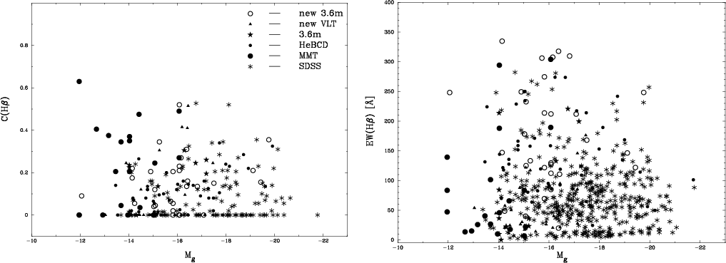 |
Figure 3:
The reddening parameter C(H |
| Open with DEXTER | |
3 Physical conditions and element abundances
The electron temperature ![]() ,
the
ionic and total heavy element abundances were derived
following Izotov et al. (2006a). In particular, for the ions
O2+, Ne2+ and Ar3+ we adopt
the temperature
,
the
ionic and total heavy element abundances were derived
following Izotov et al. (2006a). In particular, for the ions
O2+, Ne2+ and Ar3+ we adopt
the temperature ![]() (O III) directly derived from the
[O III]
(O III) directly derived from the
[O III] ![]() 4363/(
4363/(![]() 4959 +
4959 + ![]() 5007)
emission-line ratio.
For
5007)
emission-line ratio.
For ![]() (O II) and
(O II) and ![]() (S III) we use the
relation between the electron
temperatures
(S III) we use the
relation between the electron
temperatures ![]() (O III) and
the temperatures characteristic for ions O+ and S2+
obtained
by Izotov et al. (2006a) from the H II photoionization models based on recent
stellar atmosphere models and improved atomic data (Stasinska & Izotov 2003).
(O III) and
the temperatures characteristic for ions O+ and S2+
obtained
by Izotov et al. (2006a) from the H II photoionization models based on recent
stellar atmosphere models and improved atomic data (Stasinska & Izotov 2003).
We use ![]() (O II) for the calculation of
O+, N+, S+ and Fe2+ abundances and
(O II) for the calculation of
O+, N+, S+ and Fe2+ abundances and ![]() (S III)
for the calculation of S2+, Cl2+ and Ar2+ abundances.
The electron number densities for some H II regions
were obtained from the [S II]
(S III)
for the calculation of S2+, Cl2+ and Ar2+ abundances.
The electron number densities for some H II regions
were obtained from the [S II] ![]() 6717/
6717/![]() 6731 emission line
ratio. These lines were not observed or not measured in the remaining
H II regions.
For the abundance determination in those H II regions
we adopt
6731 emission line
ratio. These lines were not observed or not measured in the remaining
H II regions.
For the abundance determination in those H II regions
we adopt
![]() cm-3. The precise value of the electron number density
makes little difference in the derived abundances
since in the low-density limit which holds for the H II regions
considered here, the element abundances do not depend sensitively
on
cm-3. The precise value of the electron number density
makes little difference in the derived abundances
since in the low-density limit which holds for the H II regions
considered here, the element abundances do not depend sensitively
on ![]() .
The electron temperatures
.
The electron temperatures ![]() (O III),
(O III),
![]() (O II), the ionization correction factors (ICFs),
the ionic and total O and Ne abundances are given in
Table 5 for 3.6 m observations.
The electron temperatures
(O II), the ionization correction factors (ICFs),
the ionic and total O and Ne abundances are given in
Table 5 for 3.6 m observations.
The electron temperatures
![]() (O III),
(O III), ![]() (O II),
(O II), ![]() (S III),
electron number density
(S III),
electron number density ![]() ([S II]),
the ionization correction factors (ICFs),
the ionic and total O, N, Ne, S, Cl, Ar and Fe abundances are given in
Table 6 for VLT observations.
([S II]),
the ionization correction factors (ICFs),
the ionic and total O, N, Ne, S, Cl, Ar and Fe abundances are given in
Table 6 for VLT observations.
The oxygen abundances 12 + log O/H in 61 H II regions out of
66 obtained from the new 3.6 m ESO and VLT observations range from 7.05 to 8.22. Among them, 27 H II regions with
12 + log O/H < 7.6 are found, including 10 H II regions with
12 + log O/H < 7.3.
The combined sample consisting of the new observations, 43 BCDs from the
HeBCD sample, 30 galaxies from our previous 3.6 m ESO observations and
20 galaxies from the MMT observations yields a data set of 154 H II regions.
For comparison, we also use ![]() 9000
SDSS emission-line galaxies with the [O III]
9000
SDSS emission-line galaxies with the [O III] ![]() 4363 emission
line detected at least at the 1
4363 emission
line detected at least at the 1![]() level, allowing abundance
determination by the direct
level, allowing abundance
determination by the direct ![]() -method.
In addition, SDSS galaxies with high-quality spectra where
the [O III]
-method.
In addition, SDSS galaxies with high-quality spectra where
the [O III]![]() 4363 emission line was not detected
are used.
In the latter case, the oxygen abundances were
derived by the semiempirical method.
SDSS galaxies from the comparison sample
mostly populate the high-metallicity, high-luminosity ranges,
as compared to the galaxies from our combined sample of low-metallicity
emission-line galaxies (Figs. 5-7).
The considered galaxies span two dex in gas-phase oxygen abundance, from
4363 emission line was not detected
are used.
In the latter case, the oxygen abundances were
derived by the semiempirical method.
SDSS galaxies from the comparison sample
mostly populate the high-metallicity, high-luminosity ranges,
as compared to the galaxies from our combined sample of low-metallicity
emission-line galaxies (Figs. 5-7).
The considered galaxies span two dex in gas-phase oxygen abundance, from
![]() through
through ![]() 9.0.
9.0.
We use SDSS g magnitudes for the determination of the absolute
magnitude Mg of all galaxies from our samples,
while usually B magnitudes and MB are considered in the literature.
However, Papaderos et al. (2008) have shown that for
regions with ongoing bursts of star formation, which
is the case for our sample galaxies, the
B-g colour index is of the order of 0.1 mag only
and <0.3 mag during the first few Gyr of galactic evolution.
Therefore, we do not transform Mg to MB and directly
compare Mg's for the galaxies from our samples with
MB's for the galaxies available from the literature.
The use of the SDSS g-band photometry for all our samples allows us to
investigate the L-Z relation over the Mg range from -21 mag to the
faintest magnitude of ![]() -12 mag at the low-metallicity end.
-12 mag at the low-metallicity end.
4 Results
4.1 Luminosity-metallicity relation
In order to illustrate the main properties of our sample we plot
(a) the reddening parameter C(H![]() )
obtained from the
Balmer decrement and (b) the H
)
obtained from the
Balmer decrement and (b) the H![]() equivalent width (Fig. 3) and the logarithm
of the H
equivalent width (Fig. 3) and the logarithm
of the H![]() line luminosity (in erg s-1)
(Fig. 4) as a function of absolute magnitude Mg.
The new 3.6 m telescope and VLT data are shown by open circles and stars,
respectively.
The metal-poor galaxies collected from previous 3.6m ESO observations
are shown by filled triangles (Guseva et al. 2007; Papaderos et al. 2008).
Filled circles denote the data from the HeBCD sample collected
by Izotov et al. (2004a) and Izotov & Thuan (2004).
The MMT data (Izotov & Thuan 2007) are shown by large filled circles.
The comparison SDSS sample is represented by asterisks.
From the latter sample H II regions in
nearby spiral galaxies are excluded, as are
faint SDSS galaxies with mg > 18, the nearest
SDSS galaxies with the redshift z < 0.004 and all SDSS galaxies
with
line luminosity (in erg s-1)
(Fig. 4) as a function of absolute magnitude Mg.
The new 3.6 m telescope and VLT data are shown by open circles and stars,
respectively.
The metal-poor galaxies collected from previous 3.6m ESO observations
are shown by filled triangles (Guseva et al. 2007; Papaderos et al. 2008).
Filled circles denote the data from the HeBCD sample collected
by Izotov et al. (2004a) and Izotov & Thuan (2004).
The MMT data (Izotov & Thuan 2007) are shown by large filled circles.
The comparison SDSS sample is represented by asterisks.
From the latter sample H II regions in
nearby spiral galaxies are excluded, as are
faint SDSS galaxies with mg > 18, the nearest
SDSS galaxies with the redshift z < 0.004 and all SDSS galaxies
with ![]() [I(4363)]/
I(4363) > 0.25, totaling 443 SDSS galaxies
from the comparison sample.
[I(4363)]/
I(4363) > 0.25, totaling 443 SDSS galaxies
from the comparison sample.
Our sample does not show any trend with absolute magnitude of either
C(H![]() )
or EW(H
)
or EW(H![]() ), contrary to what was obtained by
Salzer et al. (2005) for the KISS sample.
The extinction in our sample galaxies is low. Only a few galaxies
have C(H
), contrary to what was obtained by
Salzer et al. (2005) for the KISS sample.
The extinction in our sample galaxies is low. Only a few galaxies
have C(H![]() ) > 0.4.
The range of EW(H
) > 0.4.
The range of EW(H![]() )
) ![]() 0-300
0-300 ![]() for the galaxies from
our sample is similar to that for the KISS sample
(Salzer et al. 2005) but it is higher than that for the high-redshift galaxies
of Kobulnicky et al. (2003) where EW(H
for the galaxies from
our sample is similar to that for the KISS sample
(Salzer et al. 2005) but it is higher than that for the high-redshift galaxies
of Kobulnicky et al. (2003) where EW(H![]() )
) ![]() 60
60 ![]() .
.
The logarithm of the H![]() luminosity log L(
luminosity log L(
![]() )
of our
galaxies ranges from 36 to 42 (Fig. 4).
For comparison, the galaxies from the KISS sample by Salzer et al. (2005) and
intermediate-redshift galaxies by Kobulnicky et al. (2003) have
log L(
)
of our
galaxies ranges from 36 to 42 (Fig. 4).
For comparison, the galaxies from the KISS sample by Salzer et al. (2005) and
intermediate-redshift galaxies by Kobulnicky et al. (2003) have
log L(
![]() )
) ![]() 39-43 and 39-42, respectively,
i.e. low-luminosity galaxies are lacking.
39-43 and 39-42, respectively,
i.e. low-luminosity galaxies are lacking.
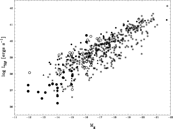 |
Figure 4:
The logarithm of the H |
| Open with DEXTER | |
In Fig. 5 we show the oxygen abundance - absolute magnitude Mgrelation for the galaxies with oxygen abundances calculated
mainly with the ![]() -method.
In this figure, the same samples and symbols as in Fig 3 are used.
The region denoted as ``branch'' is populated mainly by galaxies
with relatively high redshifts (z > 0.02) and oxygen abundances derived by
the
-method.
In this figure, the same samples and symbols as in Fig 3 are used.
The region denoted as ``branch'' is populated mainly by galaxies
with relatively high redshifts (z > 0.02) and oxygen abundances derived by
the ![]() -method.
Note that selection effects could be present for ``branch'' high-redshift
galaxies which are predominantly distant spirals. In these galaxies we select mainly
low metallicity H II regions
with a detectable [O III]
-method.
Note that selection effects could be present for ``branch'' high-redshift
galaxies which are predominantly distant spirals. In these galaxies we select mainly
low metallicity H II regions
with a detectable [O III]![]() 4363 line while the abundance
gradient is present in spirals.
The dotted line is a mean least-squares fit to all our data and the solid line
is a mean least-squares fit to our data excluding ``branch'' galaxies
with
Mg < -18.4 and systems with an oxygen abundance
in the range 8.0-8.3.
The dashed line is a mean least-squares fit to the local dwarf
irregular galaxies by Skillman et al. (1989).
Our sample (including the SDSS subsample) shows the familiar trend of
increasing metallicity with increasing luminosity.
A linear least square fit to all data yields the relation
4363 line while the abundance
gradient is present in spirals.
The dotted line is a mean least-squares fit to all our data and the solid line
is a mean least-squares fit to our data excluding ``branch'' galaxies
with
Mg < -18.4 and systems with an oxygen abundance
in the range 8.0-8.3.
The dashed line is a mean least-squares fit to the local dwarf
irregular galaxies by Skillman et al. (1989).
Our sample (including the SDSS subsample) shows the familiar trend of
increasing metallicity with increasing luminosity.
A linear least square fit to all data yields the relation
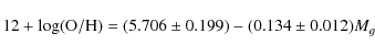 |
(1) |
(dotted line in Fig. 5). Excluding ``branch'' galaxies we obtain the relation
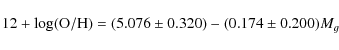 |
(2) |
(solid line in Fig. 5). We note that the Skillman et al. and Richer & McCall fits do not extend over the metallicity range of the present data. Therefore, we extrapolate the former fit in Fig. 5 (dashed line) to higher metallicities. Skillman's and our fits are obviosuly very similar. The slopes of our L-Z relation of 0.134 (0.174) are very close to the slope of 0.153 by Skillman et al. (1989) and to the slope of 0.147 by Richer & McCall (1995).
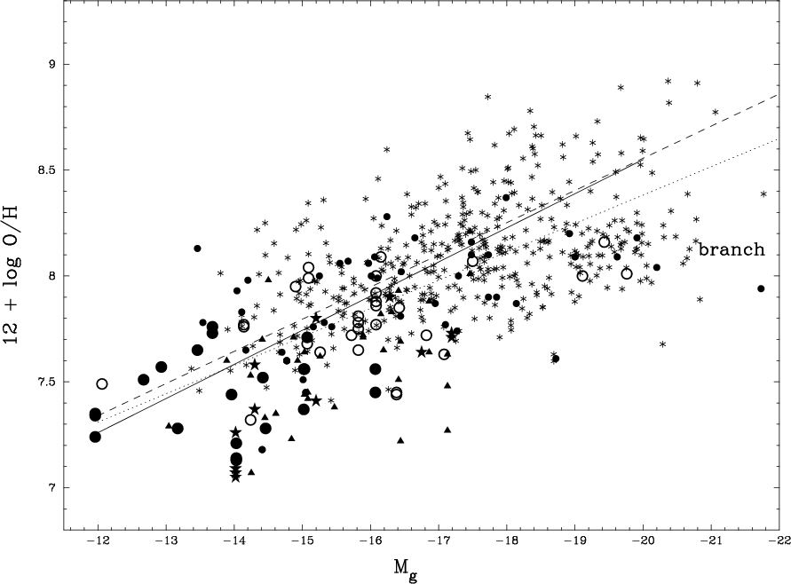 |
Figure 5:
Oxygen abundance vs. absolute magnitude for a large galaxy
sample. The same samples and symbols as in Fig. 3 are used.
The region denoted as a ``branch'' is populated mainly by the galaxies
with relatively high redshifts (z > 0.02) and oxygen abundances derived by
the |
| Open with DEXTER | |
Our sample is well populated in the low-luminosity range, while less than
10 galaxies from the KISS sample (Salzer et al. 2005)
which were used for the study of the L-Z relation
are fainter than MB = -15, and
none of them has an oxygen abundance less than 7.6.
Our sample, excluding the SDSS subsample, has a lower dispersion
around the dotted line compared to all our data and shows a shift to lower
metallicities or/and higher luminosities.
This likely can be attributed to our selection criteria which
are optimized for the search for very metal-poor emission-line galaxies.
Additionally, our sample galaxies display significant to strong
ongoing SF giving rise to a large contribution from
young stars and ionized gas to the total light of the galaxy.
Papaderos et al. (1996, see also Papaderos et al. 2002), using surface
brightness profile decomposition to separate the
star-forming component from the underlying host galaxy of BCDs,
found that SF regions provide on average 50% of the total
B-band emission within the 25 B mag/
![]() isophote,
with several examples of more intense
starbursts whose flux contribution exceeds 70%.
As a result, a shift of BCDs by a
isophote,
with several examples of more intense
starbursts whose flux contribution exceeds 70%.
As a result, a shift of BCDs by a
![]() mag with respect
to the relatively quiescent dIrr population is to be expected in
Fig. 5 (see also Fig. 9).
A similar offset to lower metallicities or/and higher luminosities has been
found by Kakazu et al. (2007) for their intermediate-redshift low-metallicity
emission-line galaxies with strong SF activity.
The mass estimate of the galaxy is less sensitive to the presence
of star-forming regions as compared to its luminosity.
This was demonstrated by Ellison et al. (2008) who found
that galaxies in close pairs show enhanced SF activity
as compared to a control sample of isolated galaxies.
At the same time galaxies in close pairs show a smaller offset in the
mass-metallicity relation as compared to the luminosity-metallicity relation.
Thus, the offset in Fig. 5 indicates that both higher luminosities and
lower metallicities may contribute to the shift in the luminosity-metallicity
diagram of our sample galaxies relative to more quiescent dIrrs.
mag with respect
to the relatively quiescent dIrr population is to be expected in
Fig. 5 (see also Fig. 9).
A similar offset to lower metallicities or/and higher luminosities has been
found by Kakazu et al. (2007) for their intermediate-redshift low-metallicity
emission-line galaxies with strong SF activity.
The mass estimate of the galaxy is less sensitive to the presence
of star-forming regions as compared to its luminosity.
This was demonstrated by Ellison et al. (2008) who found
that galaxies in close pairs show enhanced SF activity
as compared to a control sample of isolated galaxies.
At the same time galaxies in close pairs show a smaller offset in the
mass-metallicity relation as compared to the luminosity-metallicity relation.
Thus, the offset in Fig. 5 indicates that both higher luminosities and
lower metallicities may contribute to the shift in the luminosity-metallicity
diagram of our sample galaxies relative to more quiescent dIrrs.
In Fig. 6 we demonstrate that the region of ``branch''
galaxies is populated mainly by relatively high-redshift systems.
The sample is the same as in Fig. 5
but in the left panel only SDSS galaxies with oxygen abundances derived with
the ![]() -method are shown and in the right panel only relatively
high-redshift galaxies with z > 0.02 are selected.
-method are shown and in the right panel only relatively
high-redshift galaxies with z > 0.02 are selected.
The location of the galaxies on the luminosity-metallicity diagram is also
sensitive to the method used for the abundance determination.
In order to illustrate its effect on the observed L-Z relation,
we compare in Fig. 7 the oxygen abundance of SDSS sample galaxies
(dots) obtained with the direct ![]() -method (left panel) and with the
semiempirical strong-line method (right panel).
The abundances for other galaxies in Fig. 7 are the same as in Fig. 5.
In this figure we show the larger control sample of the SDSS (N=7964)
as compared to Fig. 5.
Only H II regions in nearby spiral galaxies and from the
nearest SDSS galaxies with redshifts z < 0.004 were excluded
from the
-method (left panel) and with the
semiempirical strong-line method (right panel).
The abundances for other galaxies in Fig. 7 are the same as in Fig. 5.
In this figure we show the larger control sample of the SDSS (N=7964)
as compared to Fig. 5.
Only H II regions in nearby spiral galaxies and from the
nearest SDSS galaxies with redshifts z < 0.004 were excluded
from the ![]() 9000 SDSS sources while faint galaxies with mg > 18are included.
Symbols in Fig. 7 are the same as in Fig. 3 except for SDSS
galaxies which are shown by dots.
The dotted line is a mean least-squares fit to all our data from
Fig. 5, while the solid line is a mean
least-squares fit to the same data excluding ``branch'' galaxies.
9000 SDSS sources while faint galaxies with mg > 18are included.
Symbols in Fig. 7 are the same as in Fig. 3 except for SDSS
galaxies which are shown by dots.
The dotted line is a mean least-squares fit to all our data from
Fig. 5, while the solid line is a mean
least-squares fit to the same data excluding ``branch'' galaxies.
It can be seen from Fig. 7 that the oxygen abundance of a given
galaxy obtained by different methods could differ by
![]() 0.3-0.5 dex,
especially for luminous galaxies.
This figure illus- trates clearly above
12 + log O/H
0.3-0.5 dex,
especially for luminous galaxies.
This figure illus- trates clearly above
12 + log O/H ![]() 8.5 and
Mg < -19 -20significant discrepancies between oxygen abundances
obtained from the
8.5 and
Mg < -19 -20significant discrepancies between oxygen abundances
obtained from the ![]() -method and empirical methods.
Stasinska (2002) emphasized that, at high metallicity, the
-method and empirical methods.
Stasinska (2002) emphasized that, at high metallicity, the ![]() derived from [O III]
derived from [O III] ![]() 4363 would largely overestimate
the temperature of the O++ zone (and largely underestimate the metallicity)
because cooling is dominated by the [O III]
4363 would largely overestimate
the temperature of the O++ zone (and largely underestimate the metallicity)
because cooling is dominated by the [O III] ![]() 52
52 ![]() m and
[O III]
m and
[O III] ![]() 88
88 ![]() m lines.
At the same time Pilyugin et al. (2007) demonstrated that there is
an observational limit of the highest possible metallicities
near 12 + log O/H
m lines.
At the same time Pilyugin et al. (2007) demonstrated that there is
an observational limit of the highest possible metallicities
near 12 + log O/H ![]() 8.95.
This maximum value was determined in the centers of the most luminous
(-22.3
8.95.
This maximum value was determined in the centers of the most luminous
(-22.3 ![]() MB
MB ![]() -20.3) galaxies using the
semiempirical ff-method (Pilyugin et al. 2006).
Thus, although the main mechanisms determining the electron
temperature in H II nebulae have been known for a long time,
there are still important unsolved problems.
-20.3) galaxies using the
semiempirical ff-method (Pilyugin et al. 2006).
Thus, although the main mechanisms determining the electron
temperature in H II nebulae have been known for a long time,
there are still important unsolved problems.
![\begin{figure}
\par\mbox{\includegraphics[angle=-90,width=8.5cm,clip]{12414f6a.p...
...*{5mm}
\includegraphics[angle=-90,width=8.5cm,clip]{12414f6b.ps} }\end{figure}](/articles/aa/full_html/2009/37/aa12414-09/img36.png) |
Figure 6:
The same as in Fig. 5 but ( left) only SDSS galaxies with
oxygen abundances derived with the |
| Open with DEXTER | |
The contribution of star-forming regions to the light of the galaxy can be
quantified by the equivalent width EW(H![]() )
of the H
)
of the H![]() emission line
which in turn depends on the age of the burst of star formation.
In Fig. 8 we show the same samples as in Fig. 5 except for
the SDSS galaxies now being split into two subsamples. In the
left panel only those with high equivalent widths
EW(H
emission line
which in turn depends on the age of the burst of star formation.
In Fig. 8 we show the same samples as in Fig. 5 except for
the SDSS galaxies now being split into two subsamples. In the
left panel only those with high equivalent widths
EW(H![]() ) > 80
) > 80 ![]() are shown while in the right panel only SDSS
galaxies with low equivalent widths EW(H
are shown while in the right panel only SDSS
galaxies with low equivalent widths EW(H![]() ) < 20
) < 20 ![]() are plotted.
The dotted line in the left and right panels is a
mean least-squares fit to all our data shown in Fig. 5,
while the solid line is a mean
least-squares fit to the same data excluding ``branch'' galaxies.
There is a clear difference between the two subsamples of the SDSS galaxies
by
are plotted.
The dotted line in the left and right panels is a
mean least-squares fit to all our data shown in Fig. 5,
while the solid line is a mean
least-squares fit to the same data excluding ``branch'' galaxies.
There is a clear difference between the two subsamples of the SDSS galaxies
by ![]() 0.4 dex in oxygen abundance
or, equivalently, by
0.4 dex in oxygen abundance
or, equivalently, by ![]() 3 mag in absolute magnitude.
SDSS galaxies with EW(H
3 mag in absolute magnitude.
SDSS galaxies with EW(H![]() ) > 80
) > 80 ![]() nicely follow the relation
for our dwarf low-metallicity emission-line galaxies shown as reference objects
by filled and open circles, stars, filled triangles and large filled circles.
On the other hand,
the SDSS galaxies with EW(H
nicely follow the relation
for our dwarf low-metallicity emission-line galaxies shown as reference objects
by filled and open circles, stars, filled triangles and large filled circles.
On the other hand,
the SDSS galaxies with EW(H![]() ) < 20
) < 20 ![]() are located systematically
above the low-metallicity galaxies. We propose two possible
explanations for such a difference between the two subsamples of
SDSS galaxies: 1) the emission of the SDSS galaxies with high EW(H
are located systematically
above the low-metallicity galaxies. We propose two possible
explanations for such a difference between the two subsamples of
SDSS galaxies: 1) the emission of the SDSS galaxies with high EW(H![]() )
is dominated by star-forming regions, therefore they have higher
luminosities compared to galaxies in a relatively
quiescent stage; 2) SDSS galaxies
with low EW(H
)
is dominated by star-forming regions, therefore they have higher
luminosities compared to galaxies in a relatively
quiescent stage; 2) SDSS galaxies
with low EW(H![]() )
are the ones with higher astration level, therefore they
are more chemically evolved systems with higher oxygen abundances.
Perhaps both of these explanations are tenable, accounting for the
observed differences between SDSS galaxies with high and low EW(H
)
are the ones with higher astration level, therefore they
are more chemically evolved systems with higher oxygen abundances.
Perhaps both of these explanations are tenable, accounting for the
observed differences between SDSS galaxies with high and low EW(H![]() ).
Thus, the lowest-metallicity SDSS galaxies are found predominantly among
galaxies with
high EW(H
).
Thus, the lowest-metallicity SDSS galaxies are found predominantly among
galaxies with
high EW(H![]() ).
On the other hand, no extremely low-metallicity SDSS
galaxies are found among systems with EW(H
).
On the other hand, no extremely low-metallicity SDSS
galaxies are found among systems with EW(H![]() ) < 20
) < 20 ![]() .
Thus, mixing of the SDSS galaxies with EW(H
.
Thus, mixing of the SDSS galaxies with EW(H![]() ) < 20
) < 20 ![]() and
>80
and
>80 ![]() results in a significant increase of the dispersion of the
luminosity-metallicity diagram.
results in a significant increase of the dispersion of the
luminosity-metallicity diagram.
The redshift of the galaxy could also play a role. In Fig. 5 the
bulk of the galaxies with 12 + log (O/H) = 8.0-8.3 and absolute
magnitudes between -19 and -21 mag (denoted as ``branch''
galaxies) is represented by higher-redshift
systems as compared to other galaxies from the SDSS
and a correction for redshift is required.
Since ``branch'' galaxies are blue, a correction for redshift
for systems with weak emission lines would increase
their brightness by ![]() 0.1-0.3 mag. This will not be
enough to remove the offset between ``branch'' galaxies
and lower-redshift galaxies in Fig. 5.
The situation is more complicated for ``branch'' galaxies with strong
emission lines since their effect on the apparent magnitudes of a galaxy
in standard passbands will significantly depend on redshift
(see e.g. Zackrisson et al. 2008).
Because of these reasons, we
decided not to take into account corrections for redshift.
0.1-0.3 mag. This will not be
enough to remove the offset between ``branch'' galaxies
and lower-redshift galaxies in Fig. 5.
The situation is more complicated for ``branch'' galaxies with strong
emission lines since their effect on the apparent magnitudes of a galaxy
in standard passbands will significantly depend on redshift
(see e.g. Zackrisson et al. 2008).
Because of these reasons, we
decided not to take into account corrections for redshift.
![\begin{figure}
\par\mbox{\includegraphics[angle=-90,width=8.5cm,clip]{12414f7a.p...
...*{5mm}
\includegraphics[angle=-90,width=8.5cm,clip]{12414f7b.ps} }\end{figure}](/articles/aa/full_html/2009/37/aa12414-09/img37.png) |
Figure 7:
Oxygen abundance vs. absolute magnitude. H II regions in spiral
galaxies and the nearest SDSS galaxies with
redshift z < 0.004 are excluded from the SDSS sample while faint
galaxies with
mg > 18 are included, resulting in an SDSS sample of 7964 objects.
Symbols are the same as in Fig. 3 except for SDSS galaxies which
are shown by dots. In the left panel the oxygen abundances
12 + log O/H for SDSS galaxies are obtained with the |
| Open with DEXTER | |
![\begin{figure}
\par\mbox{\includegraphics[angle=-90,width=8.5cm,clip]{12414f8a.p...
...{5mm}
\includegraphics[angle=-90,width=8.5cm,clip]{12414f8b.ps} }\end{figure}](/articles/aa/full_html/2009/37/aa12414-09/img38.png) |
Figure 8:
The same as in Fig. 5 but
only SDSS galaxies with EW(H |
| Open with DEXTER | |
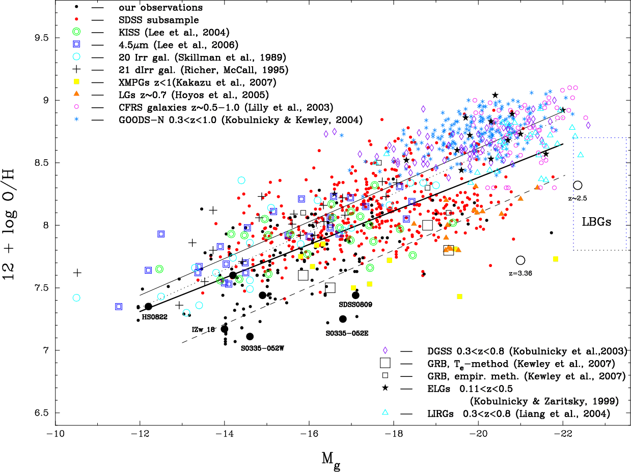 |
Figure 9: Oxygen abundance vs. absolute magnitude for the same galaxies as in Fig. 5 but all our galaxies including the SDSS sample are shown by small filled circles. Additionally, some well known metal-poor galaxies, intermediate- and high-redshift galaxies are shown by symbols as labelled in the figure. The position of the Lyman break galaxies (LBGs) by Pettini et al. (2001) is indicated by the dotted line rectangle. The thick solid line is a mean least-squares fit to all our data. The thin solid line is a least-squares fit to the data by Richer & McCall (1995) while the dotted line is a mean least-squares fit to the data by Skillman et al. (1989). The dashed line is the luminosity-metallicity relation for local metal-poor BCDs obtained by Kunth & Östlin (2000). |
| Open with DEXTER | |
4.2 Comparison of our sample with other data
In Fig. 9 we compare our L-Z relation with other
published data for galaxies of different types.
In this figure, all of our galaxies from Fig. 5, including
those from the comparison SDSS sample, are shown by small filled and open circles.
Some well known metal-poor galaxies are depicted by large filled circles and
are labelled.
Their absolute magnitudes MB are taken from Kewley et al. (2007).
For comparison, 23 KISS emission-line galaxies by
Lee et al. (2004) are displayed with large open double circles. The abundances
for these galaxies are derived with the ![]() -method,
the B-band magnitudes are from Salzer et al. (1989) and Gil de Paz et al. (2003).
With open double squares we show 25 nearby dIrrs with the 4.5
-method,
the B-band magnitudes are from Salzer et al. (1989) and Gil de Paz et al. (2003).
With open double squares we show 25 nearby dIrrs with the 4.5 ![]() m
Spitzer luminosities and compiled O/H abundances derived with
the
m
Spitzer luminosities and compiled O/H abundances derived with
the ![]() -method (Lee et al. 2006). With large open circles and large
crosses we respectively show
20 irregular galaxies from Skillman et al. (1989) and 21 dwarf irregular
galaxies from Richer & McCall (1995) for which oxygen abundances
are obtained mainly with the R23 empirical method, and for a few
objects only with the
-method (Lee et al. 2006). With large open circles and large
crosses we respectively show
20 irregular galaxies from Skillman et al. (1989) and 21 dwarf irregular
galaxies from Richer & McCall (1995) for which oxygen abundances
are obtained mainly with the R23 empirical method, and for a few
objects only with the ![]() -method.
The thick solid line is a
mean least-squares fit to all our data. The thin solid line is a
least-squares fit to the data by Richer & McCall (1995)
while the dotted line is a mean least-squares fit to the data by
Skillman et al. (1989).
The dashed line is the luminosity-metallicity relation for local
metal-poor BCDs obtained by Kunth & Östlin (2000).
-method.
The thick solid line is a
mean least-squares fit to all our data. The thin solid line is a
least-squares fit to the data by Richer & McCall (1995)
while the dotted line is a mean least-squares fit to the data by
Skillman et al. (1989).
The dashed line is the luminosity-metallicity relation for local
metal-poor BCDs obtained by Kunth & Östlin (2000).
Data for intermediate- and high-redshift galaxies are also shown.
The most distant (z < 1) extremely metal-poor galaxies (XMPGs)
(Kakazu et al. 2007) with the oxygen abundances derived with the empirical method
are shown with filled squares, while relatively metal-poor luminous galaxies
at
![]() (Hoyos et al. 2005) (O/H derived with the
(Hoyos et al. 2005) (O/H derived with the ![]() -method)
with filled triangles.
The remaining samples in Fig. 9 are the following:
a) the large open circles correspond to the z = 3.36 lensed galaxy
(Villar-Martín et al. 2004) and to the average position of luminous Lyman-break
galaxies at redshifts
-method)
with filled triangles.
The remaining samples in Fig. 9 are the following:
a) the large open circles correspond to the z = 3.36 lensed galaxy
(Villar-Martín et al. 2004) and to the average position of luminous Lyman-break
galaxies at redshifts
![]() (Kobulnicky & Koo 2000) (O/H derived
with the R23 method);
b) small open circles stand for 66 Canada-France
Redshift Survey (CFRS) galaxies by Lilly et al. (2003) in the redshift range of
(Kobulnicky & Koo 2000) (O/H derived
with the R23 method);
b) small open circles stand for 66 Canada-France
Redshift Survey (CFRS) galaxies by Lilly et al. (2003) in the redshift range of
![]() 0.5-1.0 (O/H derived with the R23 empirical method);
c) asterisks are for 204 GOODS-N (Great Observatories Origins Deep Survey -
North) emission-line galaxies in the range of redshifts 0.3 < z < 1.0
(Kobulnicky & Kewley 2004) (O/H is derived with the R23 empirical method);
d) small open rombs indicate 64 emission-line field galaxies from the
Deep Extragalactic Evolutionary
Probe Groth Strip Survey (DGSS) in the redshift range of
0.5-1.0 (O/H derived with the R23 empirical method);
c) asterisks are for 204 GOODS-N (Great Observatories Origins Deep Survey -
North) emission-line galaxies in the range of redshifts 0.3 < z < 1.0
(Kobulnicky & Kewley 2004) (O/H is derived with the R23 empirical method);
d) small open rombs indicate 64 emission-line field galaxies from the
Deep Extragalactic Evolutionary
Probe Groth Strip Survey (DGSS) in the redshift range of ![]() 0.3-0.8
(Kobulnicky et al. 2003) (O/H derived with the R23 empirical method);
e) open squares are for the gamma-ray burst (GRB) hosts by Kewley et al. (2007).
Small open squares are for galaxies with O/H derived with the empirical method
(Kewley & Dopita 2002) and large open squares for the galaxies with
O/H derived with the
0.3-0.8
(Kobulnicky et al. 2003) (O/H derived with the R23 empirical method);
e) open squares are for the gamma-ray burst (GRB) hosts by Kewley et al. (2007).
Small open squares are for galaxies with O/H derived with the empirical method
(Kewley & Dopita 2002) and large open squares for the galaxies with
O/H derived with the ![]() -method (Kewley et al. 2007);
f) filled stars denote the 14 star-forming emission-line galaxies at
intermediate redshifts (
0.11 < z < 0.5) by Kobulnicky & Zaritsky (1999)
(O/H derived with the empirical R23 method);
g) open triangles are for
29 distant 15
-method (Kewley et al. 2007);
f) filled stars denote the 14 star-forming emission-line galaxies at
intermediate redshifts (
0.11 < z < 0.5) by Kobulnicky & Zaritsky (1999)
(O/H derived with the empirical R23 method);
g) open triangles are for
29 distant 15 ![]() m-selected luminous infrared galaxies (LIRGs) at
m-selected luminous infrared galaxies (LIRGs) at
![]() -0.8 taken from the sample of Liang et al. (2004)
(O/H derived with the empirical method);
and, finally; h) the large dotted rectangle depicts the position
of Lyman break galaxies (LBGs, Pettini et al. 2001) on the L-Z diagram.
-0.8 taken from the sample of Liang et al. (2004)
(O/H derived with the empirical method);
and, finally; h) the large dotted rectangle depicts the position
of Lyman break galaxies (LBGs, Pettini et al. 2001) on the L-Z diagram.
The location of our galaxies on the luminosity-metallicity diagram is
similar to that obtained previously for local emission-line galaxies
but is shifted to higher luminosities and/or lower metallicities compared
to that obtained for quiescent irregular dwarf galaxies.
For comparison, Lee et al. (2004) have also
demonstrated that their 54 H II KISS
galaxies with O/H derived with the ![]() -method follow the L-Z relation with a slope similar to that for a more quiescent dIrrs
but are shifted to higher brightness by 0.8 mag.
Furthermore, they have shown that H II galaxies with disturbed
irregular outer
isophotes (likely due to the interaction) are shifted to a more luminous
and/or more metal-poor region in the L-Z diagram as compared to
morphologically more regular galaxies. Note that their samples of
H II galaxies and of dIrrs are in the same luminosity range
as our sample.
Papaderos et al. (2008) also note that in contrast to the majority (>90%) of
BCDs, the extremely metal-poor SF dwarfs reveal more irregular and bluer hosts.
-method follow the L-Z relation with a slope similar to that for a more quiescent dIrrs
but are shifted to higher brightness by 0.8 mag.
Furthermore, they have shown that H II galaxies with disturbed
irregular outer
isophotes (likely due to the interaction) are shifted to a more luminous
and/or more metal-poor region in the L-Z diagram as compared to
morphologically more regular galaxies. Note that their samples of
H II galaxies and of dIrrs are in the same luminosity range
as our sample.
Papaderos et al. (2008) also note that in contrast to the majority (>90%) of
BCDs, the extremely metal-poor SF dwarfs reveal more irregular and bluer hosts.
Thus, the difference in the zero point between our L-Z relation for low-metallicity galaxies and for other galaxies seems to be primarily due to the differences in the intrinsic properties of the galaxies selected for different samples with various selection criteria.
A key question is whether
a unique L-Z relation does exist for galaxies of different types.
The assessment of this issue is complicated by offsets of
high-redshift galaxies with different look-back-times.
In this context, Kobulnicky et al. (2003)
have shown that both the slopes and zero points of the
L-Z relation exhibit a smooth evolution with redshift.
A possible universal L-Z relation for galaxies is also blurred
by the fact that metallicity determinations of various galaxy samples,
differing in their EW(H![]() ), absolute magnitude and redshift, do not employ
a unique technique. More specifically,
several authors emphasize the presence of a well-known shift between
the O/H ratio obtained by the direct
), absolute magnitude and redshift, do not employ
a unique technique. More specifically,
several authors emphasize the presence of a well-known shift between
the O/H ratio obtained by the direct ![]() -method and empirical
strong-line methods.
Oxygen abundances obtained by empirical methods are by 0.1-0.25 dex
(Shi et al. 2005) and even by up to 0.6 dex (Hoyos et al. 2005) higher than
those obtained with the
-method and empirical
strong-line methods.
Oxygen abundances obtained by empirical methods are by 0.1-0.25 dex
(Shi et al. 2005) and even by up to 0.6 dex (Hoyos et al. 2005) higher than
those obtained with the ![]() -method.
For our sample we obtained an offset of
-method.
For our sample we obtained an offset of ![]() 0.3-0.5 dex.
0.3-0.5 dex.
It can be seen from Fig. 9 that the high-redshift galaxies
with an oxygen abundance derived by the ![]() -method have
a shallower slope compared to local galaxies.
On the other hand, oxygen abundances of high-redshift galaxies
obtained with the R23 empirical strong-line method
(data in Fig. 9 by Liang et al. 2004; Kobulnicky & Kewley 2004; Lilly et al. 2003) are
higher and follow the relation for high-metallicity SDSS galaxies in
Fig. 7b despite the fact that oxygen abundances for the latter
galaxies were calculated with the different semi-empirical strong-line method.
Because of this agreement we decided not to re-calculate oxygen abundances
of high-redshift galaxies with the semi-empirical method and adopted O/H
values from the literature.
Keeping in mind the systematic differences between oxygen abundances derived
with the empirical and the
-method have
a shallower slope compared to local galaxies.
On the other hand, oxygen abundances of high-redshift galaxies
obtained with the R23 empirical strong-line method
(data in Fig. 9 by Liang et al. 2004; Kobulnicky & Kewley 2004; Lilly et al. 2003) are
higher and follow the relation for high-metallicity SDSS galaxies in
Fig. 7b despite the fact that oxygen abundances for the latter
galaxies were calculated with the different semi-empirical strong-line method.
Because of this agreement we decided not to re-calculate oxygen abundances
of high-redshift galaxies with the semi-empirical method and adopted O/H
values from the literature.
Keeping in mind the systematic differences between oxygen abundances derived
with the empirical and the ![]() -methods, it might be worth
considering a decrease in oxygen abundance by
-methods, it might be worth
considering a decrease in oxygen abundance by ![]() 0.2-0.6 dex
for all high-redshift galaxies with O/H derived with the empirical method.
In that case, the position of
high-redshift galaxies on the L-Z diagram would be consistent with that of
the ``branch'' galaxies.
Such considerations add further support to the
results obtained by Pilyugin et al. (2004) and Shi et al. (2005)
that the more luminous galaxies have a slope of the L-Z relation more shallow than that of the dwarf galaxies.
0.2-0.6 dex
for all high-redshift galaxies with O/H derived with the empirical method.
In that case, the position of
high-redshift galaxies on the L-Z diagram would be consistent with that of
the ``branch'' galaxies.
Such considerations add further support to the
results obtained by Pilyugin et al. (2004) and Shi et al. (2005)
that the more luminous galaxies have a slope of the L-Z relation more shallow than that of the dwarf galaxies.
We presume that our L-Z relation could be useful as a local reference for studies of this relation for other types of local galaxies and/or of high-redshift galaxies.
5 Summary
We present VLT spectroscopic observations of a new sample of 28 H II regions from 16 emission-line galaxies and ESO 3.6 m telescope spectroscopic observations of a new sample of 38 H II regions from 28 emission-line galaxies. These galaxies have mainly been selected from the data release 6 (DR6) of the Sloan digital sky survey (SDSS) as low-metallicity galaxy candidates.
Physical conditions and element abundances are derived for 38 H II regions observed with the 3.6 m telescope and for 23 H II regions observed with the VLT.
From our new observations we find that the oxygen abundance in 61 out of the 66 observed H II in our sample ranges from 12 + log O/H = 7.05 to 8.22. The oxygen abundance in 27 H II regions is 12 + log O/H < 7.6 and among them 10 H II regions have an oxygen abundance less than 7.3.
This new data in combination with objects from our previous studies constitute a large uniform sample of 154 H II regions with high-quality spectroscopic data which are used to study the luminosity-metallicity (L-Z) relation for the local galaxies with emphasis on its low-metallicity end.
As a comparison sample we use ![]() 9000 SDSS emission-line galaxies with
higher oxygen abundances which are also obtained mainly
by the direct
9000 SDSS emission-line galaxies with
higher oxygen abundances which are also obtained mainly
by the direct ![]() -method.
For all of our sample galaxies the g magnitudes are taken from the SDSS
while the distances are from the NED.
The entire sample spans nearly two orders of magnitude
with respect to its gas-phase metallicity, from
-method.
For all of our sample galaxies the g magnitudes are taken from the SDSS
while the distances are from the NED.
The entire sample spans nearly two orders of magnitude
with respect to its gas-phase metallicity, from
![]() to
to ![]() 8.8, and covers
an absolute magnitude range from
8.8, and covers
an absolute magnitude range from
![]() to
to ![]() -20.
-20.
We find that the metallicity-luminosity relation for our galaxies is consistent with previous ones obtained for objects of similar type. The local L-Z relation obtained with high-quality spectroscopic data is useful for predictions of galaxy evolution models.
Acknowledgements
N. G. G. and Y. I. I. thank the Max Planck Institute for Radioastronomy (MPIfR) for hospitality, and acknowledge support through DFG grant No. Fr 325/57-1. P. P. thanks the Department of Astronomy and Space Physics at Uppsala University for its warm hospitality. K. J. Fricke thanks the MPIfR for Visiting Contracts during 2008 and 2009. This research was partially funded by project grant AYA2007-67965-C03-02 of the Spanish Ministerio de Ciencia e Innovacion. We acknowledge the work of the Sloan digital sky survey (SDSS) team. Funding for the SDSS has been provided by the Alfred P. Sloan Foundation, the Participating Institutions, the National Aeronautics and Space Administration, the National Science Foundation, the US Department of Energy, the Japanese Monbukagakusho, and the Max Planck Society. The SDSS Web site is http://www.sdss.org/
References
- Abazajian, K. N., Adelman-McCarthy, J. K., Agüeros, M. A., et al. 2009, ApJS, 182, 543 [NASA ADS] [CrossRef] (In the text)
- Contini, T., Treyer, M. A., Sullivan, M., & Ellis, R. S. 2002, MNRAS, 330, 75 [NASA ADS] [CrossRef]
- Ellison, S. L., Patton, D. R., Simard, L., & McConnachie, A. W. 2008, AJ, 135, 1877 [NASA ADS] [CrossRef]
- Gavilán, M., Mollá, M., & Díaz, Á. 2009, to appear in Star-forming Dwarf Galaxies: Following Ariadnes Thread in the Cosmic Labyrinth, [arXiv:0902.4695]
- Gil de Paz, A., Madore, B. F., & Pevunova, O. 2003, ApJS, 147, 29 [NASA ADS] [CrossRef] (In the text)
- Guseva, N. G., Izotov, Y. I., Papaderos, P., & Fricke, K. J. 2007, A&A, 464, 885 [NASA ADS] [CrossRef] [EDP Sciences]
- Hoyos, C., Koo, D. C., Phillips, A. C., Willmer, C. N. A., & Guhathakurta, P. 2005, ApJ, 635, L21 [NASA ADS] [CrossRef]
- Izotov, Y. I., & Thuan, T. X. 2004, ApJ, 602, 200 [NASA ADS] [CrossRef] (In the text)
- Izotov, Y. I., & Thuan, T. X. 2007, ApJ, 665, 1115 [NASA ADS] [CrossRef] (In the text)
- Izotov, Y. I., Lipovetsky, V. A., Chaffee, F. H., et al. 1997, ApJ, 476, 698 [NASA ADS] [CrossRef]
- Izotov, Y. I., Noeske, K. G., Guseva, N. G., et al. 2004a, A&A, 415, L27 [NASA ADS] [CrossRef] [EDP Sciences] (In the text)
- Izotov, Y. I., Stasinska, G., Guseva, N. G., & Thuan, T. X. 2004b, A&A, 415, 87 [NASA ADS] [CrossRef] [EDP Sciences] (In the text)
- Izotov, Y. I., Stasinska, G., Meynet, G., Guseva, N. G., & Thuan, T. X. 2006a, A&A, 448, 955 [NASA ADS] [CrossRef] [EDP Sciences] (In the text)
- Izotov, Y. I., Papaderos, P., Guseva, N. G., Fricke, K. J., & Thuan, T. X. 2006b, A&A, 454, 137 [NASA ADS] [CrossRef] [EDP Sciences]
- Kakazu, Y., Cowie, L. L., & Hu, E. M. 2007, ApJ, 668, 853 [NASA ADS] [CrossRef] (In the text)
- Kewley, L. J., & Dopita, M. A. 2002, ApJS, 142, 35 [NASA ADS] [CrossRef] (In the text)
- Kewley, L. J., Brown, W. R., Geller, M. J., Kenyon, S. J., & Kurtz, M. J. 2007, AJ, 133, 882 [NASA ADS] [CrossRef] (In the text)
- Kobulnicky, H. A., & Zaritsky, D. 1999, ApJ, 511, 118 [NASA ADS] [CrossRef]
- Kobulnicky, H. A., & Koo, D. C. 2000, ApJ, 545, 712 [NASA ADS] [CrossRef] (In the text)
- Kobulnicky, H. A., & Kewley, L. J. 2004, ApJ, 617, 240 [NASA ADS] [CrossRef] (In the text)
- Kobulnicky, H. A., Willmer, C. N. A., Phillips, A. C., et al. 2003, ApJ, 599, 1006 [NASA ADS] [CrossRef] (In the text)
- Kunth, D., & Östlin, G. 2000, Astron. Astrophys. Rev., 10, 1 [NASA ADS] [CrossRef] (In the text)
- Lamareille, F., Mouhcine, M., Contini, T., Lewis, L., & Maddox, S. 2004, MNRAS, 350, 396 [NASA ADS] [CrossRef] (In the text)
- Lee, H., Skillman, E. D., Cannon, J. M., et al. 2006, ApJ, 647, 970 [NASA ADS] [CrossRef]
- Lee, J. C., Salzer, J. J., & Melbourne, J. 2004, ApJ, 616, 752 [NASA ADS] [CrossRef]
- Lequeux, J., Rayo, J. F., Serrano, A., Peimbert, M., & Torres-Peimbert, S. 1979, A&A, 80, 155 [NASA ADS]
- Liang, Y. C., Hammer, F., Flores, H., et al. 2004, A&A, 423, 867 [NASA ADS] [CrossRef] [EDP Sciences] (In the text)
- Lilly, S. J., Carollo, C. M., & Stockton, A. N. 2003, ApJ, 597, 730 [NASA ADS] [CrossRef] (In the text)
- Maier, C., Meisenheimer, K., & Hippelein, H. 2004, A&A, 418, 475 [NASA ADS] [CrossRef] [EDP Sciences]
- Melbourne, J., & Salzer, J. J. 2002, AJ, 123, 2302 [NASA ADS] [CrossRef]
- Noeske, K. G., Papaderos, P., Cairos, L. M., & Fricke, K. J. 2003, A&A, 410, 481 [NASA ADS] [CrossRef] [EDP Sciences] (In the text)
- Papaderos, P., Loose, H.-H., Fricke, K. J., & Thuan, T. X. 1996, A&A, 314, 59 [NASA ADS] (In the text)
- Papaderos, P., Izotov, Y. I., Fricke, K. J., Thuan, T. X., & Guseva, N. G. 1998, A&A, 338, 43 [NASA ADS]
- Papaderos, P., Izotov, Y. I., Thuan, T. X., et al. 2002, A&A, 393, 461 [NASA ADS] [CrossRef] [EDP Sciences]
- Papaderos, P., Guseva, N. G., Izotov, Y. I., & Fricke, K. J. 2008, A&A, 491, 113 [NASA ADS] [CrossRef] [EDP Sciences]
- Pettini, M., Shapley, A. E., Steidel, C. C., et al. 2001, ApJ, 554, 981 [NASA ADS] [CrossRef] (In the text)
- Pilyugin, L. S., Vílchez, J. M., & Contini, T. 2004, A&A, 425, 849 [NASA ADS] [CrossRef] [EDP Sciences]
- Pilyugin, L. S., Thuan, T. X., & Vílchez, J. M. 2006, MNRAS, 367, 1139 [NASA ADS] [CrossRef] (In the text)
- Pilyugin, L. S., Thuan, T. X., & Vílchez, J. M. 2007, MNRAS, 376, 353 [NASA ADS] [CrossRef] (In the text)
- Richer, M. G., & MacCall, M. L. 1995, ApJ, 445, 642 [NASA ADS] [CrossRef]
- Salzer, J. J., MacAlpine, G. M., & Boroson, T. A. 1989, ApJS, 70, 479 [NASA ADS] [CrossRef] (In the text)
- Salzer, J. J., Lee, J. C., Melbourne, J., et al. 2005, ApJ, 624, 661 [NASA ADS] [CrossRef] (In the text)
- Saviane, I., Ivanov, V. D., Held, E. V., et al. 2008, A&A, 487, 901 [NASA ADS] [CrossRef] [EDP Sciences] (In the text)
- Shi, F., Kong, X., Li, C., & Cheng, F. Z. 2005, A&A, 437, 849 [NASA ADS] [CrossRef] [EDP Sciences]
- Skillman, E. D., Kennicutt, R. C., Jr., & Hodge, P. W. 1989, ApJ, 347, 875 [NASA ADS] [CrossRef]
- Smith, B. J., & Hancock, M. 2009, AJ, 138, 130 [NASA ADS] [CrossRef]
- Stasinska, G. 2002, RMxAC, 12, 62 [NASA ADS] (In the text)
- Stasinska, G., & Izotov, Y. I. 2003, A&A, 397, 71 [NASA ADS] [CrossRef] [EDP Sciences] (In the text)
- Thuan, T. X., & Izotov, Y. I. 2005, ApJS, 161, 240 [NASA ADS] [CrossRef] (In the text)
- Tremonti, C. A., Heckman, T. M., Kauffmann, G., et al. 2004, ApJ, 613, 898 [NASA ADS] [CrossRef]
- Vanzi, L., Hunt, L. K., Thuan, T. X., & Izotov, Y. I. 2000, A&A, 363, 493 [NASA ADS]
- Vaduvescu, O., McCall, M. L., & Richer, M. G. 2007, AJ, 134, 604 [NASA ADS] [CrossRef] (In the text)
- Vila-Costas, M. B., & Edmunds, M. G. 1992, MNRAS, 259, 121 [NASA ADS]
- Villar-Martín, M., Cerviño, M., & González Delgado, R. M. 2004, MNRAS, 355, 1132 [NASA ADS] [CrossRef] (In the text)
- Whitford, A. E. 1958, AJ, 63, 201 [NASA ADS] [CrossRef] (In the text)
- Zackrisson, E., Bergvall, N., & Leitet, E. 2008, ApJ, 676, L9 [NASA ADS] [CrossRef] (In the text)
Online Material
Table 1: List of galaxies observed with the 3.6 m ESO telescope.
Table 2: List of galaxies observed with the VLTa.
Table 3: Emission line intensities (3.6 m ESO observations).
Table 4: Emission line intensities (VLT observations).
Table 5: Ionic and total heavy element abundances (3.6 m ESO observations).
Table 6: Ionic and total heavy element abundances (VLT observations).
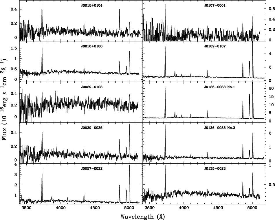 |
Figure 1: The flux-calibrated and redshift-corrected 3.6 m ESO telescope spectra of the emission-line galaxies. |
| Open with DEXTER | |
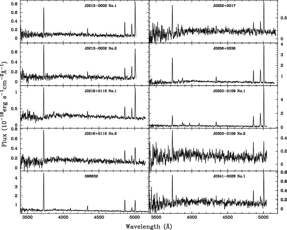 |
Figure 1: continued. |
| Open with DEXTER | |
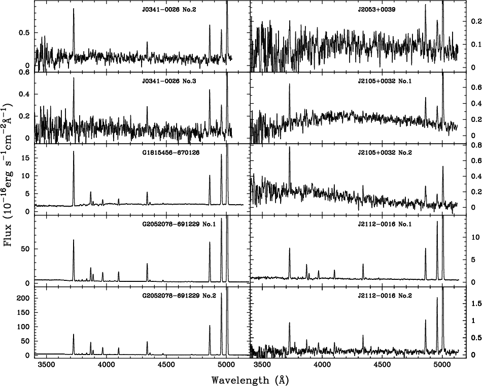 |
Figure 1: continued. |
| Open with DEXTER | |
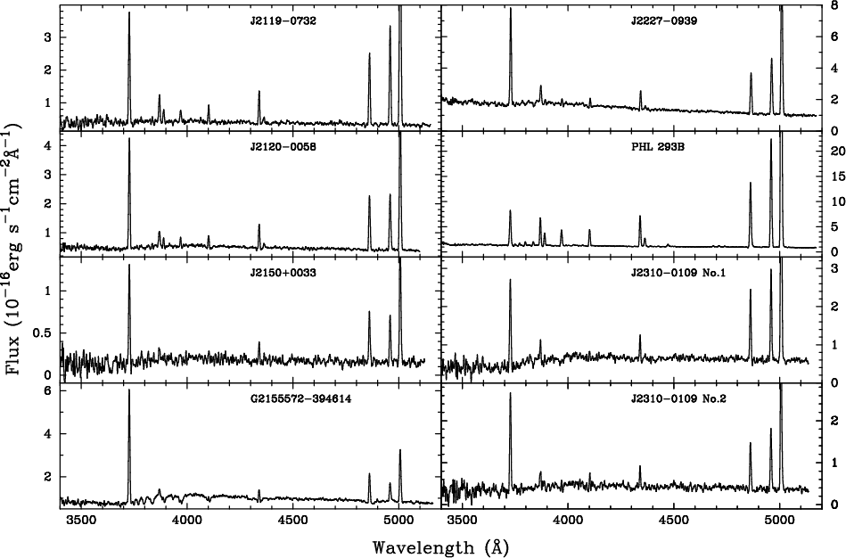 |
Figure 1: continued. |
| Open with DEXTER | |
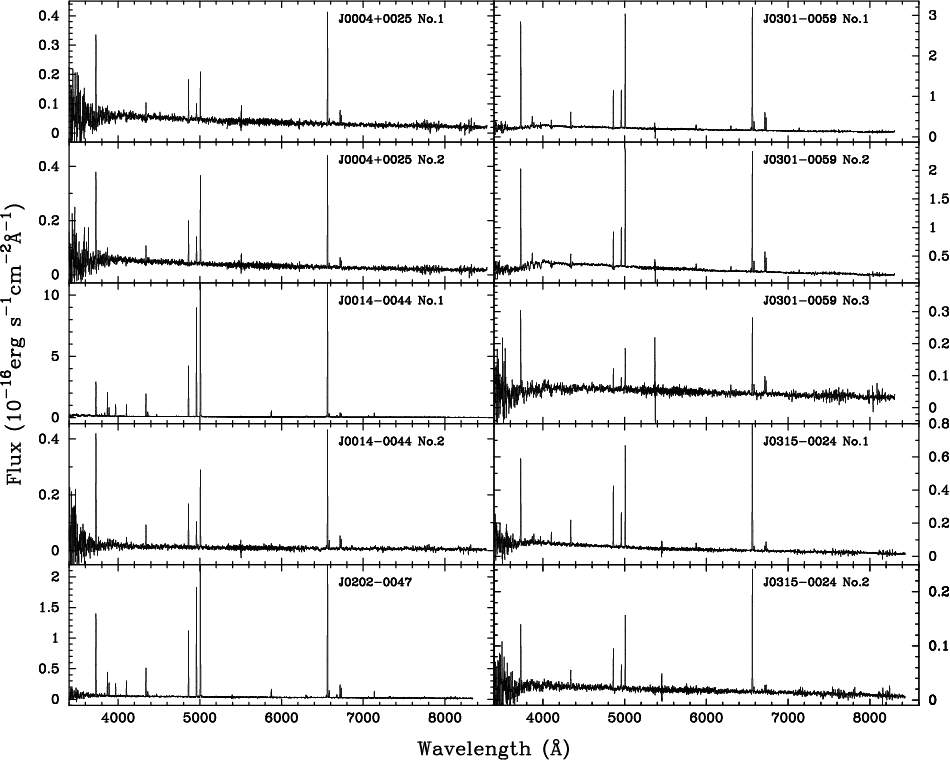 |
Figure 2: The flux-calibrated and redshift-corrected VLT spectra of the emission-line galaxies. |
| Open with DEXTER | |
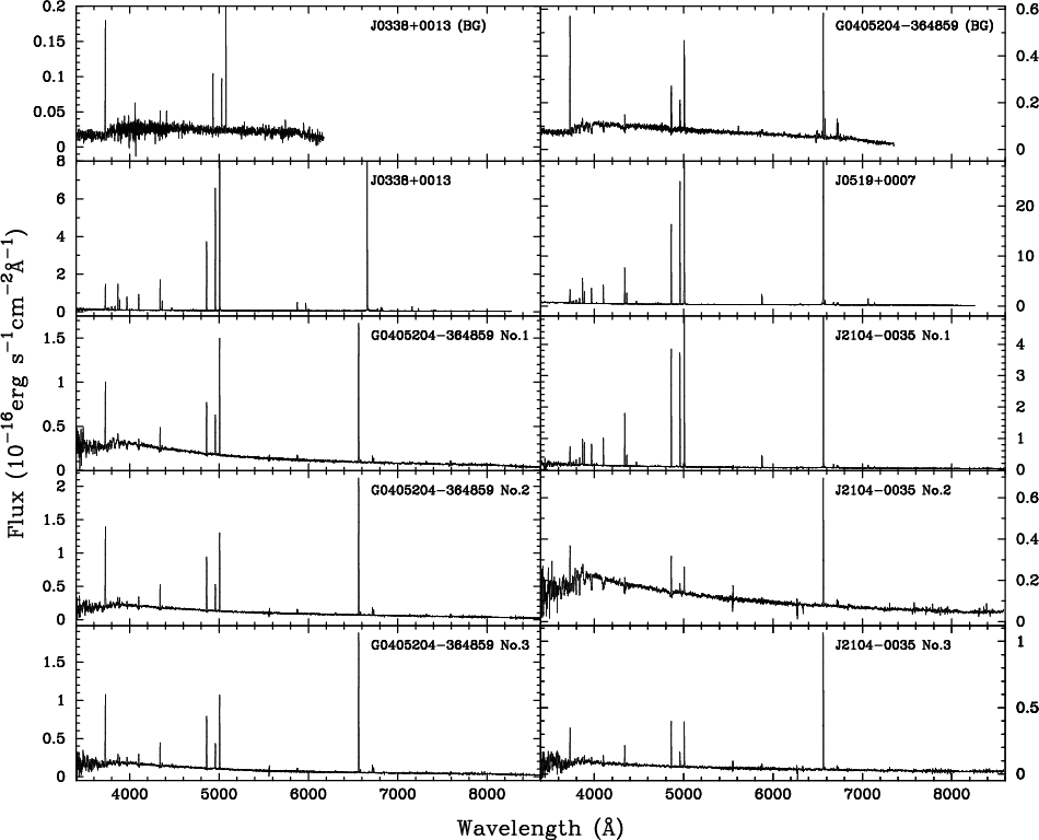 |
Figure 2: continued. |
| Open with DEXTER | |
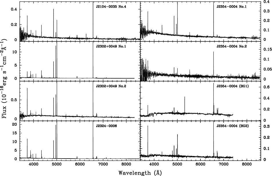 |
Figure 2: continued. |
| Open with DEXTER | |
Footnotes
- ... galaxies
- Based on observations collected at the European Southern Observatory, Chile, VLT and 3.6 m telescopes.
- ...
- Tables 1-6 and Figs. 1, 2 are only available in electronic form at http://www.aanda.org.
- ... IRAF
- IRAF is the Image Reduction and Analysis Facility distributed by the National Optical Astronomy Observatory, which is operated by the Association of Universities for Research in Astronomy (AURA) under cooperative agreement with the National Science Foundation (NSF).
All Tables
Table 1: List of galaxies observed with the 3.6 m ESO telescope.
Table 2: List of galaxies observed with the VLTa.
Table 3: Emission line intensities (3.6 m ESO observations).
Table 4: Emission line intensities (VLT observations).
Table 5: Ionic and total heavy element abundances (3.6 m ESO observations).
Table 6: Ionic and total heavy element abundances (VLT observations).
All Figures
| |
Figure 3:
The reddening parameter C(H |
| Open with DEXTER | |
| In the text | |
| |
Figure 4:
The logarithm of the H |
| Open with DEXTER | |
| In the text | |
| |
Figure 5:
Oxygen abundance vs. absolute magnitude for a large galaxy
sample. The same samples and symbols as in Fig. 3 are used.
The region denoted as a ``branch'' is populated mainly by the galaxies
with relatively high redshifts (z > 0.02) and oxygen abundances derived by
the |
| Open with DEXTER | |
| In the text | |
| |
Figure 6:
The same as in Fig. 5 but ( left) only SDSS galaxies with
oxygen abundances derived with the |
| Open with DEXTER | |
| In the text | |
| |
Figure 7:
Oxygen abundance vs. absolute magnitude. H II regions in spiral
galaxies and the nearest SDSS galaxies with
redshift z < 0.004 are excluded from the SDSS sample while faint
galaxies with
mg > 18 are included, resulting in an SDSS sample of 7964 objects.
Symbols are the same as in Fig. 3 except for SDSS galaxies which
are shown by dots. In the left panel the oxygen abundances
12 + log O/H for SDSS galaxies are obtained with the |
| Open with DEXTER | |
| In the text | |
| |
Figure 8:
The same as in Fig. 5 but
only SDSS galaxies with EW(H |
| Open with DEXTER | |
| In the text | |
| |
Figure 9: Oxygen abundance vs. absolute magnitude for the same galaxies as in Fig. 5 but all our galaxies including the SDSS sample are shown by small filled circles. Additionally, some well known metal-poor galaxies, intermediate- and high-redshift galaxies are shown by symbols as labelled in the figure. The position of the Lyman break galaxies (LBGs) by Pettini et al. (2001) is indicated by the dotted line rectangle. The thick solid line is a mean least-squares fit to all our data. The thin solid line is a least-squares fit to the data by Richer & McCall (1995) while the dotted line is a mean least-squares fit to the data by Skillman et al. (1989). The dashed line is the luminosity-metallicity relation for local metal-poor BCDs obtained by Kunth & Östlin (2000). |
| Open with DEXTER | |
| In the text | |
| |
Figure 1: The flux-calibrated and redshift-corrected 3.6 m ESO telescope spectra of the emission-line galaxies. |
| Open with DEXTER | |
| In the text | |
| |
Figure 1: continued. |
| Open with DEXTER | |
| In the text | |
| |
Figure 1: continued. |
| Open with DEXTER | |
| In the text | |
| |
Figure 1: continued. |
| Open with DEXTER | |
| In the text | |
| |
Figure 2: The flux-calibrated and redshift-corrected VLT spectra of the emission-line galaxies. |
| Open with DEXTER | |
| In the text | |
| |
Figure 2: continued. |
| Open with DEXTER | |
| In the text | |
| |
Figure 2: continued. |
| Open with DEXTER | |
| In the text | |
Copyright ESO 2009
Current usage metrics show cumulative count of Article Views (full-text article views including HTML views, PDF and ePub downloads, according to the available data) and Abstracts Views on Vision4Press platform.
Data correspond to usage on the plateform after 2015. The current usage metrics is available 48-96 hours after online publication and is updated daily on week days.
Initial download of the metrics may take a while.