Testing an exact f(R)-gravity model at Galactic and local scales

S. Capozziello; E. Piedipalumbo; C. Rubano; P. Scudellaro

doi:10.1051/0004-6361/200911992

Home

All issues

Volume 505 / No 1 (October I 2009)

A&A, 505 1 (2009) 21-28

Full HTML

Free Access

Issue		A&A Volume 505, Number 1, October I 2009


Page(s)		21 - 28
Section		Cosmology (including clusters of galaxies)
DOI		https://doi.org/10.1051/0004-6361/200911992
Published online		24 July 2009

Testing an exact f(R)-gravity model at Galactic and local scales

S. Capozziello - E. Piedipalumbo - C. Rubano - P. Scudellaro

Dipartimento di Scienze Fisiche, Università Federico II di Napoli and INFN - Sez. di Napoli, Complesso Universitario di Monte S. Angelo, via Cinthia, Ed. 6, 80126 Napoli, Italy

Received 6 March 2009 / Accepted 24 June 2009

Abstract
Context. The weak field limit for a pointlike source of a $f(R)~\propto~R^{3/2}$ -gravity model is studied.
Aims. We aim to show the viability of such a model as a valid alternative to GR + dark matter at Galactic and local scales.
Methods. Without considering dark matter, within the weak field approximation, we find general exact solutions for gravity with standard matter, and apply them to some astrophysical scales, recovering the consistency of the same f(R)-gravity model with cosmological results.
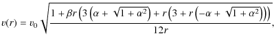
Results. In particular, we show that it is possible to obtain flat rotation curves for galaxies, and consistency with Solar System tests, as in the so-called ``Chameleon approach''. In fact, the peripheral velocity $v_\infty$ is shown to be expressed as $v_\infty = \lambda \sqrt{M}$ , so that the Tully-Fisher relation is recovered.
Conclusions. The results point out the possibility of achieving alternative theories of gravity in which exotic ingredients like dark matter and dark energy are not necessary, while their coarse-grained astrophysical and cosmological effects can be related to a geometric origin.

Key words: gravitation - Galaxy: fundamental parameters - solar system: general - cosmology: dark matter - gravitation lensing

1 Introduction

Alternative theories of gravity (Peebles & Ratra 2003; Padmanabhan 2003; Copeland et al. 2006) are increasing as possible suitable alternatives to dark energy and dark matter. Although the $\Lambda$ CDM model is affected by many theoretical shortcomings (Carroll et al. 1992), and, in general, dark energy models are mainly based on the implicit assumption that Einstein's general relativity (GR) is the correct theory of gravity. But the validity of GR both on large astrophysical and cosmological scales still remains to be accurately tested (see e.g. Will 2006), and there is still enough room to propose different theoretical schemes. A minimal alternative choice could be to take into account generic functions f(R) of the Ricci scalar curvature R. The task for these extended theories is to fit the astrophysical data without adding exotic dark ingredients (Kleinert & Schmidt 2002; Capozziello 2002; Capozziello et al. 2003a, b; Odintsov & Nojiri 2003; Carroll et al. 2004; Allemandi et al. 2004; Nojiri & Odintsov 2004; Cognola et al. 2005; Capozziello & Francaviglia 2008).

In such a context, these higher order theories have obtained considerable attention in cosmology, since they seem to work well both in the late and in the early universe (see Capozziello 2002; Capozziello et al. 2003a, b; Odintsov & Nojiri 2003; Carroll et al. 2004; Allemandi et al. 2004; Nojiri & Odintsov 2004; Cognola et al. 2005; Capozziello & Francaviglia 2008). It is also possible to show that f(R)theories can play a major role at astrophysical scales, due to the modifications of the gravitational potential in the low energy limit. Such a corrected potential reduces to the Newtonian one at the Solar System scale and could also offer the possibility of fitting galaxy rotation curves and galaxy cluster potentials without the need for large amounts of dark matter (Capozziello et al. 2004,2006,2007a,2009; Milgrom 1983, Bekenstein 2004; Sobouti 2007; Frigerio Martins & Salucci 2007; Mendoza & Rosas-Guevara 2007). However, extending the gravitational Lagrangian may give rise to many problems. These theories may have instabilities (Faraoni 2005; Cognola & Zerbini 2006; Cognola et al. 2007), ghost-like behavior (Stelle 1978), and they still need to be matched with data from the low energy limit experiments that are well understood by GR.

In summary, adopting f(R)-gravity leads to interesting results, first of all at cosmological and galactic scales, even if, up to now, it has not been possible to select only one theory (or class of theories) good at all scales. There has been much work on this (Capozziello et al. 2005; Hu & Sawicki 2007; Starobinsky 2007; Nojiri & Odintsov 2007), but all the approaches are indeed phenomenological and are not based on a fundamental conservation or invariance principle of the theory.

In this paper, we propose a specific expression of the function f(R) of the Ricci scalar curvature R, namely f(R) =-|-R|^3/2, which comes from the need for the existence of a Noether symmetry for f(R)cosmological models (de Ritis et al. 1990; Capozziello et al. 2008). The cosmological solutions of the Einstein field equations related to such a choice for f(R) have been analyzed in Capozziello et al. (2008), and it turned out that this model admits a dust-dominated decelerated phase, before a late time accelerated phase, as needed by the observational data. Here, we study the low energy limit of such a solution, in the case of a point-like source. We consider the Schwarzschild-like spherically symmetric metric in such a way that, in the weak field limit, the Newtonian potential is modified by adding a logarithmic term. A similar treatment has been proposed in Sobouti (2007), where instead the starting point consists of introducing a specific hypothesis on the metric and thereby deducing the form of f(R) (resulting in a power-law), so fitting observational data on speeds of peripheral stars in spiral galaxies, as first reported in Sanders & McGough (2002) and then selected in Sobouti (2007). Unfortunately, this procedure leads to a very peculiar choice of f(R). It contains parameters which must be adjusted to the mass of the gravitational source. Therefore, f(R) cannot be universal.

Here, we find results that are very similar to those in Sobouti (2007) from the observational point of view, but do not exhibit the above problems. In this preliminary work, we only consider the weak field generated by a point-like source. Clearly, shrinking a whole galaxy (or cluster) to a point is a very crude approximation. Our aim, therefore, is to show that the model can nonetheless work, without trying to obtain a strict correspondence with observations.

The treatment of point-like source in f(R) theories is non-trivial and, in a sense, can be considered an ill posed problem. The reason is that we cannot disregard the properties of the extended object that is generating the field. Unlike what happens in GR, the choice of the integration constants is not necessarily independent of its peculiarities, like density, equation of state etc. We should therefore solve the equations for the inner metric and then match with the exterior. This procedure is valid for a star but much less meaningful for a galaxy. In any case, we do not expect to have a full prediction of their functional dependence. In fact, also in standard GR the linear dependence on mass of the constant is obtained only from the observational link with Newtonian gravity. This link with observations is precisely what is lacking in the case of stars, and is only preliminarily studied here. Therefore, in the following we retain the assumption of point-like source, dedicating Sect. 6 to a deeper discussion on this point.

There is another limit of the analysis presented here, lying in the weak field approximation assumed from the beginning. The asymptotic Minkowskyian behavior cannot recovered and, most of all, does not shed light on the singularities of the metric. It is therefore not possible to say what are the modifications of a black hole so generated.

In Sect. 2, we work out the basic equations of our model, and in Sect. 3 we study peripheral speeds in spirals. In Sect. 4, we discuss some tests in the Solar System and, in Sect. 5, we comment on gravitational lensing and MOND. In Sect. 6 the connection between the law for a pontlike source and an extended body is briefly discussed. In Sect. 7, we give our conclusions.

2 Weak field approximation

Our theory of gravity is determined by the Action:

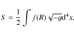
$\begin{displaymath}S=\frac{1}{2}\int{f(R)\sqrt{-g}{\rm d}^{4}x}, \end{displaymath}$

(1)

where R is the Ricci scalar and we define f(R)=-|-R|^3/2.

As said above, we consider a static, spherically symmetric metric, which will differ from the standard Schwarzschild form, due to the different starting equations. We thus set:

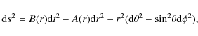
$\begin{displaymath}{\rm d}s^{2}=B(r){\rm d}t^{2}-A(r){\rm d}r^{2}-r^{2}({\rm d}{\theta}^{2}-{\sin}^{2}\theta {\rm d}\phi ^{2}), \end{displaymath}$

(2)

with A(r) and B(r) radial functions to be determined through the modified Einstein field equations.

It is important to observe that, as the angular coordinates are dimensionless, we also use a dimensionless distance, so that we have:

$\begin{displaymath}r=\rho/r_{\rm s}, \end{displaymath}$

(3)

where $\rho$ is the physical radius and $r_{\rm s}$ is a suitable scale. The choice of this scale is a delicate point: we could decide to use a universal scale or one that is specific for the particular situation. This second choice does not affect the universal character of our Action, but the situation will become clearer in the following.

Proceeding in this way, all quantities are dimensionless, including R and the result for velocities. In order to restore the appropriate dimensions, we should therefore multiply by an appropriate fundamental Action, i.e. some numerical multiple of $\hbar$ . As we are in vacuum, this clearly does not affect the equations and their solution. On the other hand, this constant is of course not irrelevant and has an influence on the coupling with the test particle (peripheral star or other object). In our case this arbitrariness will be resolved by restoring the physical units in an appropriate way when defining the observational objects and fixing the constant C₃ (see below), with the prescription that we should obtain ordinary Newtonian gravity at small scales.

In a weak field, of course, the functions A(r) and B(r) are practically identified by means of their corrections to what we expect in the Newtonian case for astrophysical situations. First trying to understand how we can modify the Newtonian potential, we write the first function as $B(r)=1-2\epsilon y(r)/r+O({\epsilon}^{2})$ , where $\epsilon$ is a suitable small parameter. Analogously, we also assume $A(r)=1+2\epsilon x(r)/r+O({\epsilon}^{2})$ . Being in a weak field, r cannot extend to infinity, but we must have $2\epsilon y(r)/r\ll1$ and $2\epsilon x(r)/r\ll1$ .

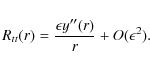
We can obtain our results depending on r, as for instance:

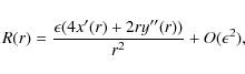
$\begin{displaymath}R(r)=\frac{\epsilon(4x^{\prime}(r)+2ry^{\prime\prime}(r))}{r^{2}}+O({\epsilon}^{2}), \end{displaymath}$

(4)

where prime denotes a derivative with respect to r. It is also:

$\begin{displaymath}R_{tt}(r)=\frac{\epsilon y^{\prime\prime}(r)}{r}+O({\epsilon}^{2}). \end{displaymath}$

(5)

To write equations, we have to vary the Action S with respect to the metric tensor, always remembering that we are studying an approximate situation. We also need to note that

$\begin{displaymath} \frac{{\rm d}f}{{\rm d}R} = \frac{3}{2}\sqrt{-\frac{4x^{\pri... ...prime\prime}(r)}{r^{2}}}\sqrt{\epsilon} + O({\epsilon}^{3/2}). \end{displaymath}$

(6)

The master equation is:

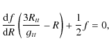
$\begin{displaymath} \frac{{\rm d}f}{{\rm d}R}\left( \frac{3R_{tt}}{g_{tt}} - R\right) + \frac{1}{2}f = 0, \end{displaymath}$

(7)

that is:

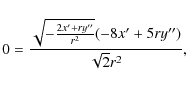
$\begin{displaymath} 0=\frac{\sqrt{-\frac{2x^{\prime}+ ry^{\prime\prime} }{r^{2}}}(-8x^{\prime}+ 5ry^{\prime\prime})}{\sqrt{2}r^{2}} , \end{displaymath}$

(8)

while the trace equation is given by:

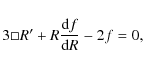
$\begin{displaymath} 3{\Box R^{\prime}} + R\frac{{\rm d}f}{{\rm d}R}- 2f = 0, \end{displaymath}$

(9)

which is equivalent to:

		$\displaystyle \left( 9\sqrt{\epsilon}\left( 4{x^{\prime\prime}}^{2} + {y^{\prim... ...+ 4x^{\prime \prime}(y^{\prime\prime}+ r y^{\prime\prime\prime})\right. \right.$
		$\displaystyle \left. \left. - 4rx^{\prime}y^{(4)} - 2ry^{\prime\prime}\left(2x^{\prime \prime\prime}+ y^{\prime\prime\prime}+ r y^{(4)}\right)\right) \right)$
		$\displaystyle \times\left( 4\sqrt{2}r^{4} \left( -\frac{2x^{\prime}+ ry^{\prime\prime}% }{r^{2}}\right) ^{3/2}\right) ^{-1} + O({\epsilon}^{3/2})=0.$	(10)

Neglecting higher order terms and dividing the master equation by ${\epsilon}^{3/2}$ and the trace equation by ${\epsilon}^{1/2}$ , we finally find

		$\displaystyle \sqrt{-\frac{2x^{\prime}+ry^{\prime\prime}}{r^{2}}}({-8x^{\prime} +5ry^{\prime\prime}})=0,$	(11)
		$\displaystyle 4{x^{\prime\prime}}^{2}+{y^{\prime\prime}}^{2}-8x^{\prime}x^{\pri... ...\prime\prime} }^{2}+4x^{\prime\prime}(y^{\prime\prime}+ry^{\prime\prime\prime})$
		$\displaystyle \hspace*{4.6mm} -~4rx^{\prime}y^{(4)}-2ry^{\prime\prime}(2x^{\prime\prime\prime} +y^{\prime\prime\prime}+ry^{(4)})=0 .$	(12)

Such equations appear only difficult to handle, since Eq. (11) can be algebraically solved for $x^{\prime}(r)$ in terms of $y^{\prime\prime}(r)$ . Discarding the solution that removes the denominator in Eq. (2.10), we are then left with

$\begin{displaymath}x^{\prime}(r)=(5/8)ry^{\prime\prime}(r). \end{displaymath}$

(13)

Substitution of this expression and its derivatives in Eq. (12) leads to the general exact solution:

y(r)	=	$\displaystyle \frac{1}{4}C_{2}r^{2}+C_{3}+C_{4}r-\frac{1}{4}C_{2}r\cos (2C_{1})$
		$\displaystyle +\frac{1}{24}C_{2}r^{3}\cos(2C_{1})+\frac{1}{4}C_{2}r\cos(2C_{1})\log r$
		$\displaystyle +\frac{1}{4}~{\rm i}~C_{2}r\sin(2C_{1})++\frac{1}{24}~{\rm i} ~C_{2}r^{3}\sin(2C_{1})$
		$\displaystyle -\frac{1}{4}~{\rm i}~C_{2}r\sin(2C_{1})\log r,$	(14)

where C₁, C₂, C₃, and C₄ are arbitrary (complex) constants. If we limit ourselves to considering C₂, C₃, and C₄ as real constants, we can understand that posing $\sin(2C_{1})=\mathbf{i} ~\alpha$ and thus $\cos(2C_{1})=\sqrt{1+{\alpha}^{2}}$ (with $\alpha \in{\rm R}$ ) makes y(r) real:

y(r)	=	$\displaystyle \frac{1}{4}C_{2}r^{2}+\frac{1}{24}C_{2}(-\alpha+\sqrt{1+{\alpha}^{2} })r^{3}+C_{3}$
		$\displaystyle +\frac{1}{4}r(-(C_{2}\alpha+C_{2}\sqrt{1+{\alpha}^{2}} -4C_{4})$
		$\displaystyle + C_{2}(\alpha+\sqrt{1+{\alpha}^{2}})\log r).$	(15)

Here, the constant C₄ is multiplied by r and, since the potential is obtained from y(r)/r, it gives rise to a constant term. So, we can set C₄=0 in the following. On the other hand, the presence of a term giving the Newtonian potential explicitly depends on C₃, which then needs to be nonzero.

From now on, $\epsilon$ will be incorporated into the integration constants without any loss of generality.

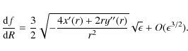
3 Peripheral speeds

We are now in a position to study how the speed of a test star behaves at the periphery of a pointlike galaxy in our model (i.e. at large distances from a point source of great mass), once it is subjected to the dimensionless potential $\Phi(r) \equiv\frac{y(r)}{r}$ . We write the speed v of a generic test star in this potential. Remembering that the quantity under the square root is dimensionless, we adjust the dimensions by means of the light speed c. This will fix the numerical values of the constants:

v(r)	$\textstyle \equiv$	$\displaystyle c\sqrt{-r\frac{{\rm d}\Phi}{{\rm d}r}}$
	=	$\displaystyle \frac{c}{2}\!\sqrt{\frac{-C_{2} r(\alpha\!\!+\!\!\sqrt{1\!+\!{\al... ...\! r(3\!+\!r(-\alpha\!+\!\!\sqrt{1\!+\!{\alpha}^{2}}))\!+\!\!12C_{3}}{3r}}\cdot$	(16)

The comparison with the Newtonian case is obtained when $\alpha=C_{2}=0.$ The value of C₃ has to be $C_{3}=\frac{GM}{c^{2}r_{\rm s}}$ . On the other hand, to get increasing velocities we need C₂ to be negative, and we define $C_{2}\equiv- {v_{0}}^{2} \beta/c^{2}$ . Defining $v_{0}\equiv\sqrt{12GM/r_{\rm s}}$ , we can then rewrite v=v(r):

$\displaystyle v(r)= v_{0}\sqrt{\frac{1+\beta r\left(3\left(\alpha+\sqrt{1+{\alp... ...ht)+r\left(3+r\left(-\alpha +\sqrt{1+{\alpha}^{2}}\right)\right)\right)}{12r}},$

(17)

with $\alpha$ and $\beta$ being dimensionless constants. Another (dimensional) constant is hidden in $r = \rho / r_{\rm s}$ . As said in Sect. 1, the value of these constants should be linked to the inner peculiarities of the body. Here, we try a much simpler procedure, and, by means of suitable guesses, try to see if there is a convenient choice that reproduces the observations. The formulation of the solution so as to have dimensionless quantities was very helpful.

The first assumption is $\alpha\gg1$ , which clearly is arbitrary and can be justified only a posteriori.

When $\alpha\gg1$ , the expression under the square root reduces to $(1/12)r^{-1}+(1/4)\beta r+(1/2)\alpha\beta$ . In fact, we find a correction of what is usually expected in the Newtonian case, since the first term is the Keplerian one, the third gives a constant speed, and the second must stay small. The reason is that, as said above, we must keep $2y(r)/r \ll1$ . This means that, even if $\alpha\gg1$ , $\beta$ must be small. However, it cannot simply be set to zero, for this would also remove the other correction term.

The second assumption is therefore that $\beta$ , being so small with respect to $\alpha$ , we can safely neglect the increasing term. A rough estimate of the relevant correction term for a galaxy is:

$\begin{displaymath}v_{\rm const}\equiv v_{0}\sqrt{\frac{1}{2}\alpha\beta}=231\sqrt{\alpha\beta}~~{\rm km~s}^{-1} \end{displaymath}$

(18)

(where we have considered $M=10^{10}~M_{\odot}$ , $r_{\rm s}=5$ Kpc, and $G\equiv G_{N}$ ), indicating that $\sqrt{\alpha\beta}\simeq1$ .

Being dimensionless quantities, $\alpha$ and $\beta$ can be universal numbers or arbitrary functions of $GM/(c^{2}r_{\rm s})$ , i.e. the only number we can form with the physical quantities at our disposal. But this is true only in the point-like source model. Another dimensionless quantity that can be considered for an extended body is of course its radius, again divided by $r_{\rm s}$ , and many others.

The third third assumption is thus that we consider $\alpha$ and $\beta$ slowly varying with respect to these kinds of parameters. In other words, we expect a difference to appear only when a very large change of scale is considered, e.g. passing from the Galaxy to the Solar System, which is discussed in Sect. 6.

The scale radius $r_{\rm s}$ , having only the function of fixing the units, can be chosen arbitrarily and we set it as a multiple of the Schwarzschild radius, $r_{\rm s}=KGM/c^{2}$ , K being an unspecified positive (large) number (if K is kept fixed, then $r_{\rm s}$ is chosen according to the first issue (see above); if, on the contrary, we want $r_{\rm s}$ to be specific, we may suitably adjust the value of K. We shall see that this makes no difference).

We thus get:

$\begin{displaymath}v^{2}(\rho)\sim\frac{6c^{2}\alpha\beta}{K}+\frac{GM}{\rho}+\frac{3c^{4}\beta }{K^{2}GM}\rho, \end{displaymath}$

(19)

that is, a constant term and a Keplerian one, plus one increasing contribution which can be neglected for sufficiently small $\beta$ and $\rho$ . This shows that the relevant parameter is the combination $\alpha\beta/K$ , while $3\beta/K^{2}$ must be negligible. We have thus reduced our problem to the determination of a unique parameter $C = \alpha \beta / K$ . We want however to stress that this simplification is due to the above assumptions. Moreover, it is clear that assumption three is more appropriately applied to C instead of its separate elements.

Any attempt to modify the Newtonian law, on the Galactic scale, has to cope with the justification of the Tully-Fisher empirical relation. This obliges one to set the parameters of the modified part as depending on the mass of the source, which is impossible if one starts from a universal modification. On the contrary, it is appropriate here, where the parameters are specific to the problem. This is indeed a very good feature of our approach. Moreover, we have complete freedom in the choice of the dependance. A reasonable assumption is to set $C= \frac{\alpha\beta}{K}$ proportional to some power of the mass M, made dimensionless by dividing by a suitable reference mass. Thus, we define $\lambda M_{1}^{n}\equiv 3\alpha\beta/K$ , where n is a pure number and M₁ is referred to $10^{10}~M_{\odot}$ . (Such a definition of $\lambda$ is the same as the one for the parameter $\alpha$ in Sobouti (2007).

$\begin{figure} \par\includegraphics[width=9cm,clip]{11992fig1} \end{figure}$	Figure 1: Fit of Eq. (21) versus data in Sanders & McGough (2002) as selected in Sobouti (2007). On the x-axis, masses of luminous matter in units of $10^{10}~M_{\odot}$ , peripheral speeds in km s^-1 in the y-axis. Error bars are not indicated as they are not reported in the reference papers. It is not crucial, since we are discussing only a preliminary estimate of the parameters.
Open with DEXTER

If we neglect the term linear in $\rho$ , we find:

$\begin{displaymath}v^{2}(\rho)\sim\frac{1}{2}c^{2}M_{1}^{n}\lambda+\frac{GM}{\rho}, \end{displaymath}$

(20)

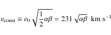
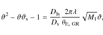
which coincides with the relevant part of the expression found in Sobouti (2007). On the other hand, the constant term can be written as:

$\begin{displaymath}v_{\rm const}=211985\cdot M_{1}^{n/2}\sqrt{\lambda}~~{\rm km~s}^{-1}. \end{displaymath}$

(21)

A determination of $\lambda$ and n can be found by fitting this formula to the data on flat rotation curves from Sanders & McGough (2002) as in Sobouti (2007), where a data list of 31 spirals is suitably selected and reported, including radii, total masses, asymptotic orbital speeds, and velocity curves for each of those galaxies. The fit is made with a non-linear regression algorithm and, as expected, we obtain the same result, as illustrated in Fig. 1. We obtain:

$\begin{displaymath}n=0.49 \pm 0.02~~~~~~~~~\lambda=(3.1\pm 0.1)\times 10^{-7}, \end{displaymath}$

(22)

compatible with n=0.5 at $1\sigma$ . This yields:

$\begin{displaymath}v~~\propto~~M^{1/4}, \end{displaymath}$

(23)

which is the phenomenological Tully-Fisher relation. We have thus proved that even in this crude model the flatness of the rotation curves can be obtained (a more detailed verification would require to treat the galaxy as an extended object); the immediate question to answer is now the validity of the theory at the Solar System level.

4 Solar System tests

4.1 Kepler's law

We now use the result of the above section for in the Solar System, with the slight simplification n = 1/2. This is a major extrapolation, as nothing guarantees that a semi-empirical law like $v^{2}(\rho)\sim(1/2)c^{2}M_{1}^{n}\lambda+GM/{\rho}$ can be used properly at such different scales, with the same values for the parameters. Possible arguments against this are:

The power law guess may be not the right one. It could indeed be more complicated and show effects at small scales.
We do not know whether $\alpha\gg1$ at the Solar System level or not.
The parameters used for the Solar System tests are those used for galaxies, and they are already roughly estimated there.
The values used for G and $M_{\odot}$ are the standard ones, which is not certain, since they are estimated within the Newtonian framework.
The orbits of the planets around the Sun are only approximately circular.
The Solar System is a many body system, where perturbations should be accurately taken into account. (The observed deviations from Kepler's laws are in fact explained by the existence of perturbations induced by other planets.)
The passage from a pointlike source to an extended one is not trivial, as said above. This point seems the most important and is treated specifically below.

If we use Eq. (20) for the calculation of the Earth's orbital speed, we find $v_{\rm Earth} = 29.8$ km s^-1, with an error of $\sim$ 1.4%, which is clearly large at this level.

In the Solar System we can also test Kepler's third law $T^{2}/{\rho}^{3}=C_{0}$ (with T the period and C₀ a constant), where:

$\begin{displaymath}T^{2}=\frac{4{\pi}^{2}{\rho}^{2}}{{v_{\rm planet}}^{2}}, \end{displaymath}$

(24)

and if we use ${v_{\rm planet}}^{2}=GM_{\odot}/\rho$ , then $C_{0}=4{\pi}^{2}/(GM_{\odot})$ . When we instead use Eq. (20) for ${v_{\rm planet}}^{2}$ , we find a non-constant result:

$\begin{displaymath}C(\rho)=\frac{4{\pi}^{2}}{GM_{\odot}+1.5\times 10^{-7}c^{2}{M}_{1/2} \rho}\cdot \end{displaymath}$

(25)

The observed values of C₀ and those obtained from Eq. (25) for Solar System planets are plotted in Fig. 2 against the semimajor axes of the planet orbits. The deviation from observation is made evident by the absence of the downwards trend, which is instead obtained from Eq. (25). However, this is not a conclusive argument, as the trend could be altered by the complicated effects of the many body system.

$\begin{figure} \par\includegraphics[width=9cm,clip]{11992fig2} \end{figure}$	Figure 2: Comparison between the values of the observed C₀s for the planets of the Solar System and what is obtained through Eq. (25). x-axis: the semi-major axes $\rho$ of the planet orbits in the Solar System (in AU units); y-axis: the observed values of C₀ (points) and the values of $C(\rho )$ computed from Eq. (25) (line).
Open with DEXTER

4.2 PPN parameter

In the study of modified (with respect to GR) approaches to gravitational physics, it is usual to ask which are the new values for the PPN parameters, in particular of the most important and studied $\gamma$ , which must be very near to 1 in the Solar System (and exactly 1 in GR).

Since we have developed our weak field approximation only up to the first order, there is some doubt about the applicability of the formalism. We have a modification of the A(r) function in the metric via the function $x(r)\neq1$ , so that we may set:

$\begin{displaymath}\gamma=x(r)=1-\frac{5\lambda c^{2}\sqrt{M_{1}}}{4GM}\rho, \end{displaymath}$

(26)

finding:

$\begin{displaymath}\gamma_{\rm earth}=0.999.\quad \end{displaymath}$

(27)

Thus, $\gamma$ turns out to be 1 up to 10^-3, which is indeed still far from the 10^-5 approximation of the Cassini experiment. Moreover, we are not able to obtain other parameters, due to the linear development in $\epsilon$ of the metric.

The reason why we do not use the conformal transformation to pass to Einstein frame is that the equivalence can be lost in the case of the weak field approximation due to the fact that a f(R)-fourth-order theory has different gauge conditions in this limit with respect to a second-order Einstein theory plus a scalar field, which could lead to unphysical results. For a detailed discussion of this point see Capozziello et al. (2007b). In order to avoid this, we adopted the Jordan frame for all calculations.

We obtain a value for $\gamma$ which is not the same throughout the Solar System. On the other hand, the numerical codes that give an estimate of the PPN parameters are based on constant values. A precise computation should instead take this feature into account. We conclude that the transport of the correction as it is at the Solar System level seems to be unsatisfactory. In Sect. 5 this problem will be addressed by the introduction of a ``Chameleon'' mechanism.

5 Other tests

Still fixing, for simplicity, n=1/2, we also set K=1 as it introduces a constant term in the potential, which is clearly irrelevant.

5.1 Gravitational lensing

Because it is intimately related to the underlying theory of gravity in its Einstein formulation, modifying the Lagrangian of the gravitational field also affects the theory of gravitational lensing. We therefore investigate how gravitational lensing works in the framework of higher order theories of gravity. On the one hand, one has to verify that the phenomenology of gravitational lensing is preserved in order to not contradict those observational results that do agree with the predictions of the standard theory of lensing. On the other hand, it is worth exploring whether deviations from classical results of the main lensing quantities could be detected and work as clear signatures of a modified theory of gravity. As a first step towards such an ambitious task, here we investigate how modifying gravity affects the gravitational lensing in the case of a point-like lens.

Indeed, the basic assumption in deriving the lens equation is that the gravitational field is weak and stationary. In this case, the spacetime metric reads:

$\begin{displaymath}{\rm d}s^2 = \left ( 1 + \frac{2 \Phi}{c^2} \right ) c^2 {\rm d}t^2 \end{displaymath}$

(28)

where $\Phi$ is the gravitational potential and, as usual, we have neglected the gravitomagnetic term. Since light rays move along the geodetics of the metric in Eq. (28), the lens equation may be simply derived by solving ds² = 0. Such a derivation holds whatever the theory of gravity is, provided that one can still write Eq. (28) in the approximation of weak and stationary fields. As a fundamental consequence, the lensing deflection angle will be given by the same formal expression found in general relativity (Schneider et al. 1992; Petters et al. 2001)

$\begin{displaymath}\vec{\alpha} = \frac{2}{c^2} \int{\vec{\nabla}_{\perp} \Phi {\rm d}l}, \end{displaymath}$

(29)

with:

$\begin{displaymath}\vec{\nabla}_{\perp} \equiv \vec{\nabla} - \hat{e} (\hat{e} {\cdot} \vec{\nabla}), \end{displaymath}$

(30)

where $\hat{e}$ is the spatial vector tangent to the direction of the light ray and d $l = \sqrt{\delta_{ij} {\rm d}x^i {\rm d}x^j}$ is the Euclidean line element. The integral in Eq. (29) should be performed along the light ray trajectory which is a priori unknown. However, for weak gravitational fields and small deflection angles, one may integrate along the unperturbed direction. In this case, we may set the position along the light ray as:

$\begin{displaymath}\vec{r} = \vec{\xi} + l \hat{e}, \end{displaymath}$

(31)

with $\vec{\xi}$ orthogonal to the light ray.

Assuming the potential only depending on $r = \vert \vec{r} \vert = (\xi^2 + l^2)^{1/2}$ (as for a point-like or a spherically symmetric lens), the deflection angle reduces to

$\begin{displaymath}\vec{\alpha} = \frac{2 \vec{\xi}}{c^2} \int_{-\infty}^{\infty... ...( \frac{1}{r} \frac{{\rm d}\Phi}{{\rm d}r} \right ) {\rm d}l}, \end{displaymath}$

(32)

where we have assumed that the geometric optics approximation holds, the light rays are paraxial and propagate from infinite distance. Equation (32) allows us to evaluate the deflection angle, provided that the source mass distribution and the theory of gravity have been assigned, so that one may determine the gravitational potential. Here, we consider only the case of the point-like lens. Note that, although being the simplest one, the point-like lens is the standard approximation for stellar lenses in microlensing applications (e.g. see Schneider et al. 1992). Moreover, since in the weak field limit $\vec{\alpha}$ is an additive quantity, the deflection angle for an extended lens may be computed integrating the point-like result weighted by the deflector surface mass distribution under the approximation of a thin lens (i.e., the mass distribution extends over a scale that is far smaller than the distances between observer, lens and source, Schneider et al. 1992). Given the symmetry of the problem, it is clear that we may deal with the magnitude of the deflection angle and of the other quantities of interest rather than with vectors.

In the approximation of small deflection angles, simple geometrical considerations allow us to write the lens equation as

$\begin{displaymath}\theta - \theta_{\rm s} = \frac{D_{\rm ls}}{D_{\rm s}} \alpha, \end{displaymath}$

(33)

which gives the position $\theta$ in the lens plane of the images of the source situated at the position $\theta_{\rm s}$ on the source plane. Note that the lens and the source planes are defined as the planes orthogonal to the optical axis, which is the line joining the observer and the center of the lens. Here and in the following, $D_{\rm l}$ , $D_{\rm s}$ , $D_{\rm ls}$ are the observer - lens, observer - source, and lens - source angular diameter distances, respectively. In order to evaluate the deflection angle, we need an explicit expression for the gravitational potential $\Phi$ generated by a pointlike mass. In our case the modified dimensional Newtonian potential, dropping unimportant constant terms and with the above assumptions, is:

$\begin{displaymath}\Phi=\frac{GM}{\rho}-2c^{2}\lambda\sqrt{M_{1}}\log\left( \frac{c^{2}\rho} {GM}\right), \end{displaymath}$

(34)

where we should remember that M₁ is measured in units of $10^{10}~M_{\odot}$ .

The first term yields, of course, the usual deviation:

$\begin{displaymath}\delta_{0} \equiv \frac{4GM}{\xi c^{2}}, \end{displaymath}$

(35)

where $\xi$ is the angular impact radius. Computing the integral $\int_{-\infty}^{+\infty}\nabla_{\bot}\Phi {\rm d}l$ leads to the additional deviation

$\begin{displaymath}\delta_{1} \equiv 2\pi\lambda\sqrt{M_{1}}, \end{displaymath}$

(36)

which is independent of $\xi$ . Now, in the case of the Sun we get

$\begin{displaymath}\delta_{0}\approx8.5\times10^{-6}~\mbox{rad\quad;}\quad\delta_{1} \approx1.7\times10^{-11}~\mbox{rad}, \end{displaymath}$

(37)

so that the correction is irrelevant. On the other hand, in the case of a galaxy, assuming M₁=1 and $\xi=10$ Kpc, we get

$\begin{displaymath}\delta_{0}\approx1.9\times10^{-6}~\mbox{rad\quad;}\quad\delta_{1} \approx 1.7\times10^{-6}~\mbox{rad}, \end{displaymath}$

(38)

so that the correction now dominates and induces an overestimation of the mass, if the deviation is instead attributed in the usual way.

The point-like lens equation differs from the standard general relativistic one for the second term (36). Should this term be negligible, all the usual results of gravitational lensing are recovered. It is therefore interesting to investigate in detail how the corrective term affects the estimate of observable related quantities since, should they be detectable, they could represent a signature of R^3/2 gravity. Since we are considering the pointlike lens, a typical lensing system is represented by a compact object (both visible or not) in the Galaxy halo acting as a lens for the light rays coming from a stellar source in an external galaxy, like the Magellanic Clouds (LMC and SMC) or Andromeda. It is easy to show that, in such a configuration, the standard Einstein angle $\theta_{\rm E,~GR}$ and the image angular separation are of the order of a few ${\times} 10^{-5}$ arcsec, so that we are in the regime known as microlensing (see Mollerach & Roulet 2002).

In the standard case the lens equation may be solved analytically and one gets two images with positions given by

$\begin{displaymath}\vartheta_{{\pm,{\rm GR}}} = \frac{1}{2} \left(\vartheta_{\rm s} {\pm} \sqrt{\vartheta_{\rm s}^2 + 4} \right) . \end{displaymath}$

(39)

In the current case, the the lens equation may be conveniently written as

$\begin{displaymath}\vartheta^2 -\vartheta \vartheta_{\rm s} - 1 = \frac{D_{\rm ... ...s}}\frac{2\pi\lambda}{\theta_{\rm E,~GR}}\sqrt{M_1}\vartheta , \end{displaymath}$

(40)

with $\vartheta = \theta/\theta_{\rm E,~GR}$ and we have defined $\theta_{\rm E,~GR}$ as the Einstein angle, which in the general relativity case is given by

$\begin{displaymath}\theta_{\rm E,~GR} = \sqrt{\frac{4 G m D_{\rm ls}}{c^2 D_{\rm l} D_{\rm s}}} . \end{displaymath}$

(41)

We still get two images on the opposite sides of the lens, with one image lying inside and the other one outside the Einstein ring. The geometric configuration is therefore the same as in the standard case, but the positions are slightly changed. The images positions are given by

$\begin{displaymath} \frac{1}{2} \left(A+\psi_\pm\sqrt{4+(A + \psi_{\rm s}^2}\right), \end{displaymath}$

(42)

with $A=2 \pi \lambda \sqrt{M_1}\frac{D_{\rm ls}}{\theta_{\rm E,~GR} D_{\rm s}}\cdot$

To quantify this effect, we evaluate the percentage deviation relative to the Einstein case. $\theta_{\rm E}=1/2 \left(A + \sqrt{4 + A^2}\right)$ , which differs from $\theta_{\rm E,~GR}$ .

5.2 Equivalence with MOND

Following Sobouti (2007), we want now to show that our model is effectively equivalent to the well known MOND theory (see Milgrom 1983; Bekenstein 2004), which postulates a modification of Newtonian dynamics:

$\begin{displaymath}F=ma\mu\left( \frac{a}{a_{0}}\right) , \end{displaymath}$

(43)

where $\mu(x)$ is a suitable function, subject to the conditions:

$\begin{displaymath}\mu(x)=1~(x\gg 1)\quad;\quad\mu(x)\rightarrow0\ (x\rightarrow0). \end{displaymath}$

(44)

F is the usual gravitational force $F=GM/\rho$ , while a₀ is a universal parameter, that regulates the transition and is estimated by means of a number of comparisons with observations, with a value $a_{0}\approx1.2\times10^{-10}$ m/s². However, the theory does not say anything about the form of the function $\mu(x)$ , which is highly degenerate.

In our case, we have that the asymptotically constant peripheral velocity $v_\infty$ can be inserted into the formula for the centripetal acceleration

$\begin{displaymath}a=\frac{v_{\infty}^{2}}{\rho}, \end{displaymath}$

(45)

so that using our expression in Eq. (20) for $v_\infty$ , we obtain

$\begin{displaymath}2a\rho=\lambda c^{2}\sqrt{\frac{M}{10^{10}~M_{\odot}}}+\frac{2GM}{\rho}, \end{displaymath}$

(46)

from which we can extract M and insert it into the expression of $\mu=\mu(a)$ . (Of course, the MOND force should now be interpreted as an effective one.)

There are two solutions, and we therefore obtain the functions:

$\displaystyle \mu_{\pm}(a/a_{0})= \frac{8aG\times 10^{10}~M_{\odot}\!+\!\lambda... ...imes 10^{10}~M_{\odot}\!+\!\lambda^{2}c^{4}}}{8aG\times 10^{10}~M_{\odot}}\cdot$

(47)

A first important remark is that $\mu$ is indeed independent of the source mass as well as of distance, and it is therefore universal, as requested. By comparison with the asymptotic limits, on the other hand, we have to choose $\mu_{-}$ and get

$\begin{displaymath}a_{0}=\frac{\lambda^{2}c^{4}}{4G\times 10^{10}~M_{\odot}}\cdot \end{displaymath}$

(48)

From the MOND estimate of a₀ we then find

$\begin{displaymath}\lambda=2.8\times 10^{-7}, \end{displaymath}$

(49)

in very good agreement with the result extracted from the above fit.

The great advantage of this formulation is that we obtain the universal function:

$\begin{displaymath}\mu(x)=\frac{1+2x-\sqrt{1+4x}}{2x}, \end{displaymath}$

(50)

which can be tested.

6 Point-like and extended bodies

As discussed in previous sections, considering the corrections to the potential from galaxies to Solar System scales, with the same values of parameters, is rather unsatisfactory. Here we want to discuss possible explanations and take into account also extended bodies.

First, both the Sun and a galaxy are not point-like sources. In the case of the Sun, however, assuming spherical symmetry and neglecting as usual the rotational contribution, we may still use the rotational invariant form of the metric in Eq. (2). There are important differences if the source is not point-like: other elements may enter in the computation of the integration constant, for instance the radius of the object. The correct treatment would be to solve for the internal metric and join it smoothly with the external one, so as to take care of the change in density with radius. A reasonable approximation would be to assume a uniform density, so that only radius could be involved. Moreover, we may consider for the moment all stars as being equal to the Sun, so that the correction to the potential can be expressed again in terms of the mass

$\begin{displaymath} \Phi=\frac{Gm}{\rho}+\mu(m)\log(\rho/r_{\rm s}). \end{displaymath}$

(51)

Here, m is the mass of the star, $r_{\rm s}$ is a scale radius, and $\mu(m)$ is a function of the mass to be determined. Since we consider all stars as being equal, $\mu$ is ``universal'' and depends on the mass only.

The situation is very different for a spiral galaxy, first, because it is not spherical and second because it is not a continuous distribution of mass. Thus, the correct procedure would be to start from a metric with cylindrical symmetry, and to solve the resulting fourth order equations. A very rough attempt would consist of computing the force acting on a test particle near the edge of the disk, by considering the galaxy as made up of, say, 10¹⁰ stars like the Sun, (without either bulge or intergalactic dust, which is indeed very crude), and adding the forces.

The force acting on a unit mass test particle is therefore

$\begin{displaymath} F=\frac{Gm}{\rho^{2}}+\frac{\mu(m)}{\rho}\cdot \end{displaymath}$

(52)

Let the test particle be situated on the x-axis, for instance (and of course on the galactic plane), R be the radius of the disk, and N the number of stars. The first term gives the usual Newtonian force, so that we only have to sum the correction. Due to the non linearity of the dependence on the mass, this is not a straightforward task. We give here just a rough estimate (a more precise computation can be made and gives the same answer).

Because of the symmetry, the total force is clearly directed towards the center, so that we need to compute only the x component. The correction is

$\begin{displaymath} \delta F=\sum\limits_{i=1}^{N}\frac{\mu(m)}{\rho_{i}}\cos(\theta_{i}), \end{displaymath}$

(53)

but, since $0<\rho_{i}<R$ and $0<\cos(\theta_{i})<1$ , we may substitute a mean value and write

$\begin{displaymath} \delta F=\sum\limits_{i=1}^{N}\chi\frac{\mu(m)}{R}=\chi N\frac{\mu(m)}{R}, \end{displaymath}$

(54)

where $\chi$ is a number of order 1. From the above discussion, on the other hand, we have seen that a good empirical expression for a galaxy is given by

$\begin{displaymath} \delta F=\frac{\lambda_{\ast}\sqrt{Nm}}{R}, \end{displaymath}$

(55)

where $\lambda_{\ast}$ is the same as the $\lambda$ used before, but in appropriate units. Comparing the two expressions we get

$\begin{displaymath} \mu(m)=\frac{\lambda_{\ast}\sqrt{Nm}}{\chi N}=\frac{\lambda_{\ast}\sqrt{m} }{\chi\sqrt{N}}\cdot \end{displaymath}$

(56)

Remembering that $\chi\sim1$ , we see that the force law for the Sun is the same that we used for a galaxy, but with a coefficient lowered by a factor $\sim$ $\sqrt{N}$ . In other words, the suppression of the correction acts in a twofold manner, because of the very low mass of the Sun compared to a galaxy, and because it is a single ``almost point-like'' object, instead of a compound one. The consequence is that all the numerical values of the local tests presented above should be lowered by a factor $\sim$ 10^-5. In this case, the approach works very well.

The main problem of this argument lies not so much in the rough estimate of $\chi$ , but in the fact that the number of stars is not the same for all galaxies, and that the stars may be very different in mass and size. A more satisfactory computation should be done starting from Eq. (52), with a reasonable guess for $\mu(m)$ (may be $\mu(m,r,...)$ ), and computing the rotation curves with the right distribution of luminous matter and number of stars. This is not a simple task and is postponed to future work.

7 Concluding remarks

Starting from a reasonably simple f(R) model for gravity, we have shown that it is possible to obtain promising astrophysical results, which do not require dark matter. What is most important is the fact that, with the same model, it appears possible to do the same also at a cosmological level, where exact solutions have been discussed preliminarily in Capozziello et al. (2008). Of course, much work has still to be done on both scales. The work here is only indicative of the concrete possibility of testing a specific f(R) model of gravity on astrophysical grounds. For cosmology, at least the structure formation and the cosmological microwave background radiation spectrum must still be investigated. On local astrophysical scales, on the other hand, more realistic models for objects like galaxies, for example, are necessary.

References

Allemandi, G., Borowiec, A., & Francaviglia, M. 2004, Phys. Rev. D, 70, 103503 [NASA ADS] [CrossRef] (In the text)
Bekenstein, J. 2004, Phys. Rev. D, 70, 083509 [NASA ADS] [CrossRef] (In the text)
Capozziello, S. 2002, Int. J. Mod. Phys. D, 11, 483 [NASA ADS] [CrossRef] (In the text)
Capozziello, S., & Francaviglia, M. 2008, GRG, 40, 357 (In the text)
Capozziello, S., Carloni, S., & Troisi, A. 2003a, Rec. Res. Dev. Astron. Astroph., 1, 1, [arXiv:astro-ph/0303041] (In the text)
Capozziello, S., Cardone, V. F., Carloni, S., & Troisi, A. 2003b, Int. J. Mod. Phys. D, 12, 1969 [NASA ADS] [CrossRef]
Capozziello, S., Cardone, V. F., Carloni, S., & Troisi, A. 2004, Phys. Lett. A, 326, 292 [NASA ADS] [CrossRef] (In the text)
Capozziello, S., Cardone, V. F., & Troisi, A. 2005, Phys. Rev. D, 71, 043503 [NASA ADS] [CrossRef] (In the text)
Capozziello, S., Cardone, V. F., & Troisi, A. 2006, JCAP, 08, 001 [NASA ADS] (In the text)
Capozziello, S., Cardone, V. F., & Troisi, A. 2007a, MNRAS, 375, 1423 [NASA ADS] [CrossRef] (In the text)
Capozzielo, S., Stabile, A., & Troisi, A. 2007b, Phys. Rev. D, 76, 104019 [NASA ADS] [CrossRef] (In the text)
Capozziello, S., Martin-Moruno, P., & Rubano, C. 2008, Phys. Lett. B, 664, 12 [NASA ADS] [CrossRef] (In the text)
Capozziello, S., De Filippis, E., & Salzano, V. 2009, MNRAS, 394, 947 [NASA ADS] [CrossRef]
Carroll, S. M., Press, W. H., & Turner, E. L. 1992, ARA&A, 30, 499 [NASA ADS] [CrossRef] (In the text)
Carroll, S. M., Duvvuri, V., Trodden, M., & Turner, M. 2004, Phys. Rev. D, 70, 043528 [NASA ADS] [CrossRef] (In the text)
Cognola, G., & Zerbini, S. 2006, J. Phys. A, 39, 6245 [NASA ADS] [CrossRef] (In the text)
Cognola, G., Elizalde, E., Nojiri, S., Odintsov, S. D., & Zerbini, S. 2005, JCAP, 010 (In the text)
Cognola, G., Gastaldi, M., & Zerbini, S. 2008, Int. J. Theor. Phys., 47, 898 [CrossRef] (In the text)
Copeland, E. J., Sami, M., & Tsujikawa, S. 2006, Int. J. Mod. Phys. D, 15, 1753 [NASA ADS] [CrossRef] (In the text)
de Ritis, R., Marmo, G., Platania, G., et al. 1990, Phys. Rev. D, 42, 1091 [NASA ADS] [CrossRef] (In the text)
Faraoni, V. 2005, Phys. Rev. D, 72, 124005 [NASA ADS] [CrossRef] (In the text)
Frigerio Martins, C., & Salucci, P. 2007, MNRAS, 381, 1103 [NASA ADS] [CrossRef] (In the text)
Hu, W., & Sawicki, I. 2007, Phys. Rev. D, 76, 064004 [NASA ADS] [CrossRef] (In the text)
Kleinert, H., & Schmidt, H.-J. 2002, GRG, 34, 1295 (In the text)
Mendoza, S., & Rosas-Guevara, Y. M. 2007, A&A, 472, 367 [NASA ADS] [CrossRef] [EDP Sciences] (In the text)
Milgrom, M. 1983, ApJ, 270, 365 [NASA ADS] [CrossRef] (In the text)
Mollerach, S., & Roulet, E. 2002, Gravitational lensing and microlensing (Singapore: World Scientific Publisher) (In the text)
Nojiri, S., & Odintsov, S. D. 2004, GRG, 36, 1765 (In the text)
Nojiri, S., & Odintsov, S. D. 2007, Phys. Lett. B, 652, 343 [NASA ADS] [CrossRef] (In the text)
Odintsov, S. D., & Nojiri, S. 2003, Phys. Lett. B, 576, 5 [NASA ADS] [CrossRef] (In the text)
Padmanabhan, T. 2003, Phys. Rep., 380, 235 [NASA ADS] [CrossRef] (In the text)
Peebles, P. J. E., & Rathra, B. 2003, Rev. Mod. Phys., 75, 559 [NASA ADS] [CrossRef] (In the text)
Petters, A. O., Levine, H., & Wambsganss, J. 2001, Singularity theory and gravitational lensing (Boston: Birkhauser) (In the text)
Sanders, R. H., & McGough, S. S. 2002, ARA&A, 40, 263 [NASA ADS] [CrossRef] (In the text)
Schneider, P., Ehlers, J., & Falco, E. E. 1992, Gravitational lenses (Berlin: Springer-Verlag) (In the text)
Sobouti, Y. 2007, A&A, 464, 921 [NASA ADS] [CrossRef] [EDP Sciences] (In the text)
Starobinsky, A. A. 2007, JETP Lett., 86, 157 [NASA ADS] [CrossRef] (In the text)
Stelle, K. S. 1978, GRG, 9, 353 (In the text)
Will, C. M. 2006, Living Rev. Relativity, 9, [arXiv:gr-qc/0510072] (In the text)

Footnotes

... namely: where the combination of minus signs is only due to our conventions, since we start from the metric (- + + +) and we obtain R < 0and $G_{\rm eff} = - 1/f^{\prime}$ .
... vector: Here, quantities in boldface are vectors, while the versor will be denoted by an over-hat.
... plane: Both $\theta$ and $\theta_{\rm s}$ are measured in angular units and could be redefined as $\theta = \xi/D_{\rm l}$ and $\theta_{\rm s} = \eta/D_{\rm s}$ with $\xi$ and $\eta$ in linear units.
... way: Here, we limit ourselves to observing that, of course, the actual computation should be much more complicated, not only because of the fact that a galaxy is an extended object, but also because of the necessity to recompute the cosmological angular diameter distances.

All Figures

$\begin{figure} \par\includegraphics[width=9cm,clip]{11992fig1} \end{figure}$	Figure 1: Fit of Eq. (21) versus data in Sanders & McGough (2002) as selected in Sobouti (2007). On the x-axis, masses of luminous matter in units of $10^{10}~M_{\odot}$ , peripheral speeds in km s^-1 in the y-axis. Error bars are not indicated as they are not reported in the reference papers. It is not crucial, since we are discussing only a preliminary estimate of the parameters.
Open with DEXTER
In the text

$\begin{figure} \par\includegraphics[width=9cm,clip]{11992fig2} \end{figure}$	Figure 2: Comparison between the values of the observed C₀s for the planets of the Solar System and what is obtained through Eq. (25). x-axis: the semi-major axes $\rho$ of the planet orbits in the Solar System (in AU units); y-axis: the observed values of C₀ (points) and the values of $C(\rho )$ computed from Eq. (25) (line).
Open with DEXTER
In the text

Current usage metrics show cumulative count of Article Views (full-text article views including HTML views, PDF and ePub downloads, according to the available data) and Abstracts Views on Vision4Press platform.

Data correspond to usage on the plateform after 2015. The current usage metrics is available 48-96 hours after online publication and is updated daily on week days.

Initial download of the metrics may take a while.