| Issue |
A&A
Volume 504, Number 3, September IV 2009
|
|
|---|---|---|
| Page(s) | 1057 - 1070 | |
| Section | The Sun | |
| DOI | https://doi.org/10.1051/0004-6361/200912341 | |
| Published online | 16 July 2009 | |
Stationary and impulsive injection of electron beams in converging magnetic field
T. V. Siversky - V. V. Zharkova
Department of Mathematics, University of Bradford, Bradford BD7 1DP, UK
Received 16 April 2009 / Accepted 5 June 2009
Abstract
Aims. We study time-dependent precipitation of an electron beam injected into a flaring atmosphere with a converging magnetic field by considering collisional and Ohmic losses with anisotropic scattering and pitch angle diffusion. Two injection regimes are investigated: short impulse and stationary injection. The effects of converging magnetic fields with different spatial profiles are compared and the energy deposition produced by the precipitating electrons at different depths and regimes is calculated.
Methods. The time dependent Fokker-Planck equation for electron distribution in depth, energy and pitch angle was solved numerically by using the summary approximation method.
Results. Steady state injection was found to be established for beam electrons 0.07-0.2 s after the injection onset depending on the initial beam parameters. Energy deposition by a stationary beam is strongly dependent on a self-induced electric field but more weakly dependent on a magnetic field convergence. Energy depositions by short electron impulses are found to be insensitive to the self-induced electric field but are strongly affected by magnetic convergence. Short beam impulses are shown to produce sharp asymmetric hard X-ray bursts on a timescale of the order of tens of milliseconds, often observed in solar flares.
Key words: Sun: atmosphere - Sun: flares - Sun: X-rays, gamma rays - scattering - radiation mechanisms: non-thermal - X-rays: bursts
1 Introduction
Observations of solar flares in hard X-rays provide vital information about scenarios in which accelerated electrons gain and deposit their energy into flaring atmospheres. The theory describing the generation of bremsstrahlung emission has progressed significantly in many directions by improving the mechanisms for emitting this radiation, e.g., considering relativistic bremsstrahlung cross-sections (Kontar et al. 2006), taking into account various aspects of the photospheric albedo effects, while deriving mean electron spectra from the observed bremsstrahlung photon spectra (Kontar et al. 2006). On the other hand, substantial improvements have also been made in solving the direct problem of electron precipitation into a flaring atmosphere by taking into account different mechanisms of electron energy losses: Coulomb collisions (Brown et al. 2000; Brown 1971) combined with deceleration by the self-induced electric field (Zharkova et al. 1995; Zharkova & Gordovskyy 2006) in flaring atmospheres with strong temperature and density gradients derived from hydrodynamic solutions (Fisher et al. 1985; Somov et al. 1982,1981; Nagai & Emslie 1984).
Substantial progress in the quantitative interpretation of hard X-ray emission has been achieved by using high temporal and spatial resolution observations carried out by the RHESSI payload (Lin et al. 2003). These observations infer the locations and shapes of hard X-ray sources on the solar disk, their temporal variations, and energy spectra evolution during the flare duration (Krucker et al. 2008; Holman et al. 2003). These observations are often accompanied by other observations (in microwaves (MW), EUV, and optical ranges), which identify a very close temporal correlation between HXR and MW, UV, and even optical emission (see for example, Kundu et al. 2004; Grechnev et al. 2008; Fletcher et al. 2007. This has highlighted the further need for improvements in electron transport models, which can simultaneously account both temporarily and spatially for all these types of emission.
The RHESSI observations of double power law energy spectra, which exhibit flattening towards lower photon energies (Holman et al. 2003) leading to the soft-hard-soft temporal pattern of the photon spectra indices below
![]() (Grigis & Benz 2006), highlighted the role of a self-induced electric field of beam electrons in their spectral flattening (Zharkova & Gordovskyy 2006). The authors considered a stationary beam injection and naturally reproduced the spectral flattening by means of electron deceleration in the electric field, induced by beam electrons themselves. The flattening was shown to be proportional to the initial energy flux of beam electrons and their spectral indices (Zharkova & Gordovskyy 2006). The soft-hard-soft pattern in photon spectra above can then be easily reproduced by a triangular increase and decrease in the beam energy flux within a time interval of a few seconds, which was often observed both by RHESSI (Lin et al. 2003), and by the previous SMM mission (Kane et al. 1980). Furthermore, numerous observations of solar flares by SMM, TRACE, and RHESSI suggest that the areas of flaring loops decrease and, thus, their magnetic fields increase with the depth of the solar atmosphere (Lang et al. 1993; Kontar et al. 2008; Brosius & White 2006). This increase in magnetic field can act as a magnetic mirror for the precipitating electrons that, in addition to the effect of self-induced electric field, forces them to return to their source in the corona.
(Grigis & Benz 2006), highlighted the role of a self-induced electric field of beam electrons in their spectral flattening (Zharkova & Gordovskyy 2006). The authors considered a stationary beam injection and naturally reproduced the spectral flattening by means of electron deceleration in the electric field, induced by beam electrons themselves. The flattening was shown to be proportional to the initial energy flux of beam electrons and their spectral indices (Zharkova & Gordovskyy 2006). The soft-hard-soft pattern in photon spectra above can then be easily reproduced by a triangular increase and decrease in the beam energy flux within a time interval of a few seconds, which was often observed both by RHESSI (Lin et al. 2003), and by the previous SMM mission (Kane et al. 1980). Furthermore, numerous observations of solar flares by SMM, TRACE, and RHESSI suggest that the areas of flaring loops decrease and, thus, their magnetic fields increase with the depth of the solar atmosphere (Lang et al. 1993; Kontar et al. 2008; Brosius & White 2006). This increase in magnetic field can act as a magnetic mirror for the precipitating electrons that, in addition to the effect of self-induced electric field, forces them to return to their source in the corona.
In the present paper, we propose two models of magnetic field variations with depth. One model fits measurements of the magnetic field in the corona (Brosius & White 2006) and chromosphere (Kontar et al. 2008), another shows the exponential increase in the magnetic field from the corona to the upper chromosphere, while retaining a constant value in the lower chromosphere. The outcome is compared with those of the two other models proposed earlier: the first one (Leach & Petrosian 1981), where the authors assumed that the magnetic column depth scale
![]() is constant implying that there is an exponential magnetic field increase with column depth, and the second one (McClements 1992) including a parabolic increase in the magnetic field with linear depth.
is constant implying that there is an exponential magnetic field increase with column depth, and the second one (McClements 1992) including a parabolic increase in the magnetic field with linear depth.
The temporal intervals of impulsive increases in HXR emission also vary from very short tens of milliseconds (Kiplinger et al. 1983; Charikov et al. 2004) to tens of minutes as often observed by RHESSI (Holman et al. 2003). This encouraged us to revise the electron transport models and consider solutions of a time-dependent Fokker-Planck equation for different timescales of beam injection (milliseconds, seconds, and minutes). The electron transport, in turn, can also be deaccelerated by anisotropic scattering of beam electrons in this self-induced electric field enhanced by the magnetic mirroring of the same electrons in converging magnetic loops. The additional delay can be caused by the particle diffusion in pitch angles and energy, which can significantly extend the electron transport time into deeper atmospheric layers where they are fully thermalised.
We also apply the time dependent Fokker-Planck equation to compare the solutions for electron precipitation for stationary and impulsive injection and their effect on resulting hard X-ray emission and ambient plasma heating for different parameters of beam electrons. We also investigate these Fokker-Planck solutions for the different models of a converging magnetic field by taking into account all the mechanisms of energy loss (collisions and Ohmic losses) and anisotropic scattering but without diffusion of energy.
The problem is formulated in Sect. 2, and the method of solution is described in Sect. 3. The stationary injection into a flaring atmosphere with different magnetic field convergence and collisional plus Ohmic losses with anisotropic scattering is considered in Sect. 4, and the impulsive injection on short timescales below tens milliseconds is considered in Sect. 5. The discussion and conclusions are drawn in Sect. 6.
2 Problem formulation
2.1 The Fokker-Planck equation
We consider a one-dimensional beam of high energy electrons injected into the solar atmosphere. The beam electron velocity distribution f, as a function of time t, depth l, velocity V, and pitch angle between the velocity and the magnetic field ![]() ,
can be found by solving the Fokker-Planck equation (Diakonov & Somov 1988; Zharkova et al. 1995)
,
can be found by solving the Fokker-Planck equation (Diakonov & Somov 1988; Zharkova et al. 1995)
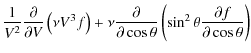
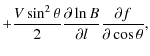
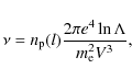
where the collisional rate
 |
(2) |
We introduce the following dimensionless variables:
| |
= |  |
(3) |
| s | = |  |
(4) |
| z | = |  |
(5) |
| = | (6) | ||
| = | (7) | ||
| n | = | (8) |
where
 |
(9) |
where
 |
(11) |
As shown by van den Oord (1990), after a few collisional times from the start of the beam injection, the background plasma fully compensates for the charge and current deposited by the beam. In our model, we assume that the beam current is always compensated, i.e.,
where the dimensionless conductivity is
and
![\begin{figure}\par\includegraphics[width=9cm,clip]{pics/12341fg1.eps}
\end{figure}](/articles/aa/full_html/2009/36/aa12341-09/img52.png) |
Figure 1:
Density and temperature of the ambient plasma calculated by the hydro-dynamic model (Zharkova & Zharkov 2007) for different beam energy flux, F0, and power law index, |
| Open with DEXTER | |
The electron beam and the plasma return current can be a subject of various plasma instabilities. For example, Zharkova & Kobylinskij (1992) demonstrated that a beam with energy flux higher than
![]() can be unstable with respect to the ion-sound waves. However, these instabilities are beyond the scope of the current paper and will be considered in forthcoming studies.
can be unstable with respect to the ion-sound waves. However, these instabilities are beyond the scope of the current paper and will be considered in forthcoming studies.
2.2 Initial and boundary conditions
There are no beam electrons before the injection starts, thus, the initial condition is
| (14) |
The boundary condition at
where
 |
(16) |
is equal to some preset value
| (17) |
The distribution function is calculated for the following range of energies:
 = 0, = 0, |
(18) |
 = 0. = 0. |
(19) |
The boundary conditions on pitch angle are (McClements 1990)
 = 0, = 0, |
(20) |
 = 0. = 0. |
(21) |
2.3 Integral characteristics of the electron distribution in the beam
Before numerically solving Eq. (10), we define the following quantities of the electron beam that we propose to calculate: beam density (in
![]() ),
),
 |
(22) |
differential particle flux spectrum (in
 |
(23) |
mean particle flux spectrum (in
 |
(24) |
angle distribution (in arbitrary units),
 |
(25) |
and energy deposition (or heating function) of the beam (in
 |
(26) |
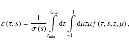
where dz/ds is the electron's energy losses with depth, which can be estimated as (Emslie 1980)
 |
(27) |
where two terms represent the collisional and Ohmic energy losses respectively. Coefficient
3 The summary approximation method
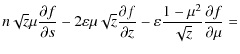
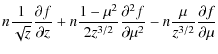
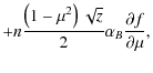
We combine the relative derivatives and rewrite the Fokker-Planck equation of Eq. (10) in the following form:
Equation (28) is solved numerically by using the summary approximation method (Samarskii 2001). This method allows us to study the time dependent Fokker-Planck equation and differs from the one used by Zharkova & Gordovskyy (2005b) to solve the stationary problem. According to the summary approximation method, the four-dimensional problem is reduced to a chain of three two-dimensional problems. This is achieved by considering the three-dimensional differential operator on the right-hand side of Eq. (10) as a sum of one-dimensional operators, each acting on the distribution function separately during one third of the time step. At each time substep, the distribution function is calculated implicitly, hence, the numerical scheme is
where
Equation (29) together with boundary conditions forms a set of linear equations, which, after being solved, infers
![]() from known
from known ![]() .
The distribution function
.
The distribution function
![]() is then used in Eq. (30) to obtain
is then used in Eq. (30) to obtain
![]() .
Finally, from Eq. (31) we obtain
.
Finally, from Eq. (31) we obtain
![]() ,
which is, in turn, used in Eq. (29) in the next step.
,
which is, in turn, used in Eq. (29) in the next step.
Electric field
![]() is calculated for each time step according to Eq. (12), where the distribution function is taken from the previous step. Thus, the numerical scheme is not fully implicit. This means that to avoid numerical instability, the time step,
is calculated for each time step according to Eq. (12), where the distribution function is taken from the previous step. Thus, the numerical scheme is not fully implicit. This means that to avoid numerical instability, the time step,
![]() ,
must be shorter than some critical value
,
must be shorter than some critical value
![]() .
In practice, the time step was determined by the trial-and-error method. For example, for the energy flux
.
In practice, the time step was determined by the trial-and-error method. For example, for the energy flux
![]() the time step is
the time step is
![]() .
It was found that when the energy flux is increased, the time step had to decrease proportionally to keep the numerical scheme stable.
.
It was found that when the energy flux is increased, the time step had to decrease proportionally to keep the numerical scheme stable.
4 Stationary injection
We first recapture the major simulation results for the case of a stationary (steady) injection, which helps us to understand the physical process of energy losses by beam electrons during their precipitation. In Zharkova et al. (2009), we studied hard X-ray emission and polarisation produced by a steady beam, while in the current paper we focus more on comparing electron precipitation results obtained for different models of magnetic convergence and on the energy deposition at various depths and times by electron beams with different parameters.
The electron injection starts at t=0 and the simulation continues until the stationary state is reached. The initial spectral index of the beam is chosen to be
![]() ,
the energy flux at the top boundary is
,
the energy flux at the top boundary is
![]() ,
and the initial angle dispersion is
,
and the initial angle dispersion is
![]() .
.
4.1 Relaxation time to a steady injection
We first show how the system relaxes to the stationary state. Figure 2 shows the profiles of the electric field and beam density at different times. It can be seen that the electric field relaxes more rapidly than the density. The relaxation time ![]() ,
after which the system becomes stationary, can be estimated to be
,
after which the system becomes stationary, can be estimated to be ![]()
![]() .
As stated in Sect. 2.1, the self-induced electric field is calculated based on the assumption that the beam current changes on timescales longer than the plasma collisional time. Since the collisional time in the corona is about
.
As stated in Sect. 2.1, the self-induced electric field is calculated based on the assumption that the beam current changes on timescales longer than the plasma collisional time. Since the collisional time in the corona is about
![]() and decreases with depth, we may conclude that this assumption is correct.
and decreases with depth, we may conclude that this assumption is correct.
It was found that this relaxation time is longer for a stronger beam, which is the result of a lower ambient plasma density (Fig. 1) and, hence, a larger linear depth for the same column depth. For example, the depth
![]() corresponds to
corresponds to
![]() and
and
![]() for the beam energy fluxes
for the beam energy fluxes
![]() and
and
![]() ,
respectively. This leads to a longer relaxation time for the atmosphere preheated by a stronger beam, e.g., for the beam energy flux of
,
respectively. This leads to a longer relaxation time for the atmosphere preheated by a stronger beam, e.g., for the beam energy flux of
![]() ,
the relaxation time is found to be
,
the relaxation time is found to be ![]()
![]() .
.
![\begin{figure}
\par\subfigure[]{\includegraphics[width=9cm,clip]{pics/12341fg2a....
...ubfigure[]{\includegraphics[width=9cm,clip]{pics/12341fg2b.eps} }
\end{figure}](/articles/aa/full_html/2009/36/aa12341-09/img126.png) |
Figure 2:
Electron density a) and self-induced electric field b) profiles, where t is time passed after the injection is ``turned on''. Collisions and electric field are taken into account. The beam parameters (see Eq. (15)) are
|
| Open with DEXTER | |
4.2 Effects of collisions and electric field (
 )
)
![\begin{figure}
\par\includegraphics[width=9cm,clip]{pics/12341fg3.eps}
\end{figure}](/articles/aa/full_html/2009/36/aa12341-09/img127.png) |
Figure 3: Beam electron density in different energy bands, if only collisions are taken into account. Beam parameters are the same as in Fig. 2. |
| Open with DEXTER | |
The local maximum, which appears in the density profile for a depth of about ![]()
![]() (Fig. 2a), is caused by beam deceleration, while the flux of electrons remains nearly constant. After this depth, most of the electrons leave the distribution (thermalise) by reducing their energy below the energy
(Fig. 2a), is caused by beam deceleration, while the flux of electrons remains nearly constant. After this depth, most of the electrons leave the distribution (thermalise) by reducing their energy below the energy
![]() ,
and the density rapidly decreases at a depth of about
,
and the density rapidly decreases at a depth of about ![]()
![]() (Fig. 2a). This corresponds to the stopping depth for electrons with energies close to the lower cut-off energy (
(Fig. 2a). This corresponds to the stopping depth for electrons with energies close to the lower cut-off energy (
![]() ). The electrons with higher energies can travel deeper (see Fig. 3). In particular, it can be seen that electrons with energies >
). The electrons with higher energies can travel deeper (see Fig. 3). In particular, it can be seen that electrons with energies >
![]() can travel down to the photosphere almost without any energy losses. Figure 3 confirms the results obtained by Zharkova & Gordovskyy (2006, see their Table 1).
can travel down to the photosphere almost without any energy losses. Figure 3 confirms the results obtained by Zharkova & Gordovskyy (2006, see their Table 1).
The depth profile of the electric field (Fig. 2b) has some noticeable variations at column depths of about
![]() ,
,
![]() ,
and
,
and
![]() .
These features are located at the same depths where the temperature profile (Fig. 1) exhibits sharp decreases leading to the sharp decreases in plasma conductivity given by Eq. (13). However, the electron density fluctuation associated (through the Gauss's Law) with this electric field profile is found to be of the order of
.
These features are located at the same depths where the temperature profile (Fig. 1) exhibits sharp decreases leading to the sharp decreases in plasma conductivity given by Eq. (13). However, the electron density fluctuation associated (through the Gauss's Law) with this electric field profile is found to be of the order of
![]() and can be neglected.
and can be neglected.
In Fig. 4, we plot the differential flux spectra at different depths for the forward (![]() )
and backward (
)
and backward (![]() )
moving electrons. It can be seen that the self-induced electric field does not change the spectra of the downward (
)
moving electrons. It can be seen that the self-induced electric field does not change the spectra of the downward (![]() )
moving electrons but affects only the spectra of the upward (
)
moving electrons but affects only the spectra of the upward (![]() )
moving ones. Since the pitch angle diffusion due to the electric field is more effective for lower energy electrons, the spectra of the returned electrons is enhanced at low and mid energy (Fig. 4d).
)
moving ones. Since the pitch angle diffusion due to the electric field is more effective for lower energy electrons, the spectra of the returned electrons is enhanced at low and mid energy (Fig. 4d).
The number of electrons returning back to the source plotted in Fig. 5a is lower than when the self-induced electric field is not taken into account. However, even without the electric field
![]() ,
a number of electrons with
,
a number of electrons with ![]() is essential owing to the pitch angle scattering (second and third terms on the right hand side of Eq. (10)).
is essential owing to the pitch angle scattering (second and third terms on the right hand side of Eq. (10)).
The heating function plot (Fig. 5b) shows that if a self-induced electric field is taken into account the heating is more effective at an upper column depth (
![]() )
than a much lower one (
)
than a much lower one (
![]() )
in the pure collisional beam relaxation, which is consistent with the results obtained by Emslie (1980). Indeed, the inclusion of the electric field decreases the stopping depth (Zharkova & Gordovskyy 2006) and increases the number of returning electrons, thus, reducing the number of electrons at larger depths. All these factors lead to an upward shift in the heating function maximum. The theoretical heating curve for pure collisions (Syrovatskii & Shmeleva 1972) is plotted in Fig. 5b.
)
in the pure collisional beam relaxation, which is consistent with the results obtained by Emslie (1980). Indeed, the inclusion of the electric field decreases the stopping depth (Zharkova & Gordovskyy 2006) and increases the number of returning electrons, thus, reducing the number of electrons at larger depths. All these factors lead to an upward shift in the heating function maximum. The theoretical heating curve for pure collisions (Syrovatskii & Shmeleva 1972) is plotted in Fig. 5b.
![\begin{figure}
\par\mbox{\subfigure[collisions, $\mu>0$ ]{\includegraphics[width...
...<0$ ]{
\includegraphics[width=8.3cm,clip]{pics/12341fg4d.eps} }}
\end{figure}](/articles/aa/full_html/2009/36/aa12341-09/img136.png) |
Figure 4: Differential flux spectra of the beam electrons integrated over the positive and negative pitch angles. Beam parameters are the same as in Fig. 2. |
| Open with DEXTER | |
![\begin{figure}
\par\subfigure[]{\includegraphics[width=9cm,clip]{pics/12341fg5a....
...ubfigure[]{\includegraphics[width=9cm,clip]{pics/12341fg5b.eps} }
\end{figure}](/articles/aa/full_html/2009/36/aa12341-09/img137.png) |
Figure 5: Pitch angle distribution a) and heating function of the beam b). Beam parameters are the same as in Fig. 2 and the magnetic convergence (for dotted curve) is given by Eq. (36). |
| Open with DEXTER | |
4.3 Effects of a magnetic convergence
![\begin{figure}
\par\includegraphics[width=9cm,clip]{pics/12341fg6.eps}
\end{figure}](/articles/aa/full_html/2009/36/aa12341-09/img138.png) |
Figure 6: The ratio of the dimensionless electric field to the ambient plasma density as a function of column depth. Collisions and electric field are taken into account. Beam parameters are the same as in Fig. 2. |
| Open with DEXTER | |
![\begin{figure}
\par\subfigure[]{\includegraphics[width=9cm,clip]{pics/12341fg7a....
...ubfigure[]{\includegraphics[width=9cm,clip]{pics/12341fg7b.eps} }
\end{figure}](/articles/aa/full_html/2009/36/aa12341-09/img139.png) |
Figure 7:
Mean flux spectra a) of the upward ( |
| Open with DEXTER | |
The converging magnetic field acts as a magnetic mirror and can increase the number of the electrons that move upwards. We determine how large the magnetic convergence parameter,
![]() ,
should be to have any noticeable effect on the distribution of beam electrons. To do so, we compare the terms in front of the
,
should be to have any noticeable effect on the distribution of beam electrons. To do so, we compare the terms in front of the
![]() symbol in Eq. (28). Since the collisional pitch angle diffusion is much lower than the one caused by the electric field (see Fig. 5a), we compare the effects of the magnetic convergence with those caused by the electric field. The magnetic convergence effects are stronger if
symbol in Eq. (28). Since the collisional pitch angle diffusion is much lower than the one caused by the electric field (see Fig. 5a), we compare the effects of the magnetic convergence with those caused by the electric field. The magnetic convergence effects are stronger if
![]() .
To estimate this expression, we plot the dimensionless ratio
.
To estimate this expression, we plot the dimensionless ratio
![]() in Fig. 6. The minimal value of the ratio
in Fig. 6. The minimal value of the ratio
![]() in the interval from
in the interval from
![]() to the stopping depth of low energy (z=1) electrons,
to the stopping depth of low energy (z=1) electrons, ![]()
![]() ,
is about 0.2. Thus, the magnetic convergence would be more effective than the electric field for the electrons with energies higher than the cut-off energy if
,
is about 0.2. Thus, the magnetic convergence would be more effective than the electric field for the electrons with energies higher than the cut-off energy if
![]() .
High energy electrons can travel much deeper into the chromosphere (see Fig. 3), where the ratio
.
High energy electrons can travel much deeper into the chromosphere (see Fig. 3), where the ratio
![]() can be as low as
can be as low as
![]() ,
thus the magnetic convergence would be more effective for them if
,
thus the magnetic convergence would be more effective for them if
![]() .
.
In the following subsections, we present the results of simulations for different models of the converging magnetic field. These results are illustrated by the mean flux spectra plots (Fig. 7a) for the upward (![]() )
moving electrons, while the spectra of the downward moving electrons are found to be very close for all convergence models. The energy deposition profiles for different magnetic field approximations are shown in Fig. 7b.
)
moving electrons, while the spectra of the downward moving electrons are found to be very close for all convergence models. The energy deposition profiles for different magnetic field approximations are shown in Fig. 7b.
4.3.1 Exponential approximation of a magnetic field convergence
Following the approximation proposed by Leach & Petrosian (1981), we assume that the convergence parameter does not depend on depth
and that then the magnetic field variation is given by
We assume that the magnetic field at the depth
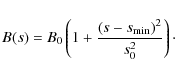
4.3.2 Parabolic approximation
McClements (1992) suggested the following profile of a magnetic field variation:
If
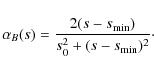
The magnetic convergence parameter
4.3.3 Hybrid approximation of magnetic field
![\begin{figure}
\par\subfigure[convergence]{\includegraphics[width=8.5cm,clip]{pi...
...lisions]{\includegraphics[width=8.5cm,clip]{pics/12341fg8b.eps} }
\end{figure}](/articles/aa/full_html/2009/36/aa12341-09/img158.png) |
Figure 8: Beam electron density in different energy bands. The magnetic convergence parameter is given by Eq. (36). Beam parameters are the same as in Fig. 2. |
| Open with DEXTER | |
![\begin{figure}
\par\subfigure[]{\includegraphics[width=9cm,clip]{pics/12341fg9a....
...ubfigure[]{\includegraphics[width=9cm,clip]{pics/12341fg9b.eps} }
\end{figure}](/articles/aa/full_html/2009/36/aa12341-09/img159.png) |
Figure 9:
Beam density a) and energy deposition b) as a function of column depth. The magnetic convergence parameter is given by Eq. (36) with various
|
| Open with DEXTER | |
In this model, we propose that
![]() is almost constant at small depth (in the corona) and tends to zero after some depth s0 (in the chromosphere)
is almost constant at small depth (in the corona) and tends to zero after some depth s0 (in the chromosphere)
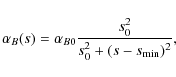
and the magnetic field variation is then
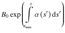
At shallow depths, where
Electrons with velocities inside the loss-cone are not reflected by the magnetic mirror and reach deeper layers. For the current convergence model, the critical pitch angle cosine of the loss-cone is
![]() .
This means that for the accepted initial angle dispersion of 0.2, about
.
This means that for the accepted initial angle dispersion of 0.2, about ![]() of the electrons are reflected back.
of the electrons are reflected back.
As can be seen in Fig. 5b, the effect of magnetic convergence on the pitch angle distribution is similar to the effect of the electric field. However, since the electric field is most effective for the electrons with ![]() ,
the pitch angle distribution reaches a maximum at
,
the pitch angle distribution reaches a maximum at ![]() when convergence is not taken into account. In contrast, the magnetic field does not affect electrons moving along the field lines, thus, the angle distribution of the upward moving electrons has a maximum at
when convergence is not taken into account. In contrast, the magnetic field does not affect electrons moving along the field lines, thus, the angle distribution of the upward moving electrons has a maximum at
![]() (Fig. 5a), which is consistent with the conclusions of Zharkova & Gordovskyy (2006).
(Fig. 5a), which is consistent with the conclusions of Zharkova & Gordovskyy (2006).
Since the convergence parameter
![]() is relatively high in this model, the entire spectrum of electron energy is affected (see Fig. 7a). The energy deposition profile for this magnetic field approximation (Fig. 7b) indicates that the heating is only about
is relatively high in this model, the entire spectrum of electron energy is affected (see Fig. 7a). The energy deposition profile for this magnetic field approximation (Fig. 7b) indicates that the heating is only about ![]() of the heating produced in the case of constant magnetic field, which is because many electrons are reflected by the magnetic mirror before they enter the dense plasma.
of the heating produced in the case of constant magnetic field, which is because many electrons are reflected by the magnetic mirror before they enter the dense plasma.
The profiles of electron density for different energies are plotted in Fig. 8. If only magnetic convergence is taken into account (Fig. 8a), it can be seen that magnetic mirroring does not depend on the electron energy. Electrons whose pitch angles are outside the loss-cone are turned back at a depth ![]()
![]() .
The remaining electrons (the pitch angles of which are inside the loss-cone) can travel down to the lower boundary of the atmosphere. When collisions are taken into account, electrons, especially those with low energies, lose their energy due to collisions (Fig. 8b). It is important to compare collisional beam relaxation with and without magnetic convergence as plotted in Figs. 8b and 3, respectively. It is noticeable that the combination of the effects of collisions and convergence is stronger than the sum of the two separate effects. This occurs because electrons with the initial pitch angles inside the loss-cone are scattered by collisions to pitch angles that fall out of the loss-cone, therefore, more electrons are returned back by the magnetic mirror.
.
The remaining electrons (the pitch angles of which are inside the loss-cone) can travel down to the lower boundary of the atmosphere. When collisions are taken into account, electrons, especially those with low energies, lose their energy due to collisions (Fig. 8b). It is important to compare collisional beam relaxation with and without magnetic convergence as plotted in Figs. 8b and 3, respectively. It is noticeable that the combination of the effects of collisions and convergence is stronger than the sum of the two separate effects. This occurs because electrons with the initial pitch angles inside the loss-cone are scattered by collisions to pitch angles that fall out of the loss-cone, therefore, more electrons are returned back by the magnetic mirror.
In Fig. 9, the results of simulations are presented for different magnitudes for the parameters
![]() and s0 of the magnetic convergence model given by Eq. (36). The increase in
and s0 of the magnetic convergence model given by Eq. (36). The increase in
![]() clearly affects the beam electrons by reducing the depth of their penetration and by increasing the number of returning electrons. It is obvious that the system would be sensitive to the variation in s0, if it is smaller than the penetration (stopping) depth. This is proven in Fig. 9a.
clearly affects the beam electrons by reducing the depth of their penetration and by increasing the number of returning electrons. It is obvious that the system would be sensitive to the variation in s0, if it is smaller than the penetration (stopping) depth. This is proven in Fig. 9a.
4.3.4 Magnetic field model fitted to the observations
Although the magnetic field cannot be directly measured in the solar atmosphere, there are some indirect techniques that allow the magnitude of the magnetic field to be estimated. The coronal magnetic field can be determined from radio observations of gyro-resonance emission (Lang et al. 1993; Brosius & White 2006). In particular, Brosius & White (2006) suggest that the magnetic scale height above sunspots,
![]() ,
is
,
is ![]()
![]() .
On the other hand, Kontar et al. (2008) determined the chromospheric magnetic field by measuring the sizes and heights of hard X-ray sources in different energy bands. They found that the chromospheric magnetic scale height,
.
On the other hand, Kontar et al. (2008) determined the chromospheric magnetic field by measuring the sizes and heights of hard X-ray sources in different energy bands. They found that the chromospheric magnetic scale height,
![]() ,
is
,
is ![]()
![]() .
Assuming that the magnetic scale height, LB, changes linearly with depth l, the convergence parameter is
.
Assuming that the magnetic scale height, LB, changes linearly with depth l, the convergence parameter is

where
 |
(40) |
where the linear depth is
As can be seen in Fig. 7a, this magnetic convergence affects electrons of all energies. This leads to about a ![]() reduction in the heating produced by beam electrons in comparison to the constant magnetic field profile (Fig. 7b).
reduction in the heating produced by beam electrons in comparison to the constant magnetic field profile (Fig. 7b).
![\begin{figure}
\par\subfigure[]{\includegraphics[width=9cm,clip]{pics/12341fg10a...
...cludegraphics[width=9cm,clip]{pics/12341fg10b.eps} }\vspace{-2mm}
\end{figure}](/articles/aa/full_html/2009/36/aa12341-09/img188.png) |
Figure 10:
Electron density at impulsive injection as a function of column depth a) and pitch angle b). Collisions and the electric field are taken into account. The beam parameters, see Eq. (15), are |
| Open with DEXTER | |
5 Impulsive injection
We now consider the precipitation of electron beam injected as a short impulse. The early SMM (Kiplinger et al. 1983) and CORONAS/IRIS (Charikov et al. 2004) observations identify millisecond impulses in the hard X-ray emission from solar flares. Furthermore, the electron acceleration time in a reconnecting current sheet was shown by Siversky & Zharkova (2009) to be as short as
![]() .
The timescale of a beam of accelerated electrons should therefore be rather short. In this section, we study the evolution in these short impulses in the solar atmosphere. The injection time,
.
The timescale of a beam of accelerated electrons should therefore be rather short. In this section, we study the evolution in these short impulses in the solar atmosphere. The injection time, ![]() ,
is chosen to be
,
is chosen to be
![]() ,
which is much shorter than the relaxation time
,
which is much shorter than the relaxation time
![]() ,
found in Sect. 4.1 (see Fig. 2). The default parameters of the beam are similar to those for stationary injection: the initial spectral index of the beam is
,
found in Sect. 4.1 (see Fig. 2). The default parameters of the beam are similar to those for stationary injection: the initial spectral index of the beam is
![]() ,
the maximal energy flux at the top boundary is
,
the maximal energy flux at the top boundary is
![]() ,
and the initial angle dispersion is
,
and the initial angle dispersion is
![]() .
The energy deposition profiles produced both by a softer beam (
.
The energy deposition profiles produced both by a softer beam (
![]() )
and by a stronger beam (
)
and by a stronger beam (
![]() )
are also obtained.
)
are also obtained.
The impulse injection, obviously, leads to a lower density of electrons at a given depth in comparison with the stationary injection (see Figs. 2a and 10a). A lower density produces a lower self-induced electric field. Thus, in the case of a short impulsive injection, the electric field does not affect the distributions so much. As a result, the only mechanism that can increase the number of returning electrons is magnetic convergence. As mentioned above in the current study, we assume that the beam current is always compensated by the plasma return current, thus the self-induced electric field develops immediately. However, as shown by van den Oord (1990), the neutralisation time of the beam current is of the order of the collisional time. Thus, the effect of the electric field on short impulses can be even smaller than our estimations.
Anisotropic scattering of beam electrons in collisions with the ambient plasma causes the pitch angle distribution to become flatter with time (see Fig. 10b). The electrons propagating downward reach depths of high ambient plasma density, lose their energy due to collisions, and leave the distribution (becoming thermalised) when their energy is less than
![]() .
In contrast, the returning electrons move into less dense plasma almost without losing any energy, but gaining energy in the self-induced electric field. Thus, after some time the number of upward moving electrons can exceed the number of downward moving ones, which is clearly seen in Fig. 10b. The angle distributions show that after
.
In contrast, the returning electrons move into less dense plasma almost without losing any energy, but gaining energy in the self-induced electric field. Thus, after some time the number of upward moving electrons can exceed the number of downward moving ones, which is clearly seen in Fig. 10b. The angle distributions show that after ![]()
![]() ,
most of the downward propagating electrons are gone and the majority of electrons have
,
most of the downward propagating electrons are gone and the majority of electrons have ![]() ,
i.e., they move back to their source in the corona.
,
i.e., they move back to their source in the corona.
![\begin{figure}% latex2html id marker 1097\par\mbox{\subfigure[collisions]{\inc...
...:conv4})]{
\includegraphics[width=8.5cm]{pics/12341fg11d.eps} }}
\end{figure}](/articles/aa/full_html/2009/36/aa12341-09/img195.png) |
Figure 11: Mean flux spectra of the electrons injected as a short impulse. The beam parameters are the same as in Fig. 10. |
| Open with DEXTER | |
5.1 Energy spectra
Since the first term in the right-hand side of Eq. (10), which is responsible for the energy losses due to collisions, is proportional to z-1/2 (where z is the dimensionless energy), one might expect that electron spectra would become harder with time. However, the downward moving electrons of higher energy both reach the dense plasma and lose their energy faster than lower energy electrons, which makes the energy spectra softer with time (Fig. 11a). The same is valid for the spectra of the upward moving electrons. In this case, the high energy electrons escape the distribution faster by reaching the top boundary (
![]() ). Because of this effect, the power law index can increase from the initial value of 3, to 4 during the beam evolution (Fig. 11a).
). Because of this effect, the power law index can increase from the initial value of 3, to 4 during the beam evolution (Fig. 11a).
![\begin{figure}
\par\mbox{\subfigure[collisions]{
\includegraphics[width=8.5cm,c...
...eld]{
\includegraphics[width=8.5cm,clip]{pics/12341fg12d.eps} }}
\end{figure}](/articles/aa/full_html/2009/36/aa12341-09/img196.png) |
Figure 12: Energy deposition by a beam impulse. The beam parameters are the same as in Fig. 10 and the magnetic convergence is given by Eq. (36). |
| Open with DEXTER | |
A magnetic field on its own cannot change the energy of the electrons. However, a converging magnetic field acts as a magnetic mirror and returns most of the electrons back to their source. As shown above in Fig. 7a, for the high energy electrons the magnetic convergence is more effective than the electric field and pitch angle diffusion. Thus, high energy electrons can quickly escape through the
![]() boundary and the power law index can reach higher values than for a constant magnetic field. For example, for the magnetic field profile given by Eq. (37) the power law index increases from the initial value of 3 to 8 (Fig. 11c). If the convergence parameter is defined by Eq. (39), the initial power law distribution converts to some kind of quasi-thermal distribution with drop at high energies (Fig. 11d).
boundary and the power law index can reach higher values than for a constant magnetic field. For example, for the magnetic field profile given by Eq. (37) the power law index increases from the initial value of 3 to 8 (Fig. 11c). If the convergence parameter is defined by Eq. (39), the initial power law distribution converts to some kind of quasi-thermal distribution with drop at high energies (Fig. 11d).
![\begin{figure}
\par\subfigure[collisions]{
\includegraphics[width=8.8cm,clip]{p...
...eld]{
\includegraphics[width=8.8cm,clip]{pics/12341fg13b.eps} }
\end{figure}](/articles/aa/full_html/2009/36/aa12341-09/img210.png) |
Figure 13:
Energy deposition by the impulse of a beam with |
| Open with DEXTER | |
![\begin{figure}
\par\subfigure[collisions]{\includegraphics[width=8.8cm,clip]{pic...
...gence]{\includegraphics[width=8.8cm,clip]{pics/12341fg14c.eps} }
\end{figure}](/articles/aa/full_html/2009/36/aa12341-09/img198.png) |
Figure 14:
Energy deposition of the beam impulse with the energy flux
|
| Open with DEXTER | |
5.2 Energy deposition
Figure 12 shows the evolution in the energy deposition, or heating functions, when different precipitation effects are taken into account. In the purely collisional case (Fig. 12a), the heating maximum appears at the bottom boundary, moves upwards with time and vanishes near column depths of ![]()
![]() .
This evolution is consistent with stopping depths obtained for electrons with different energies (Fig. 3). The high energy electrons are the first to reach depths where the density is high enough to thermalise them. Less energetic electrons travel longer because of their lower velocity but lose their energy higher in the atmosphere. Thus, the heating function maximum moves with precipitation time from the photosphere (
.
This evolution is consistent with stopping depths obtained for electrons with different energies (Fig. 3). The high energy electrons are the first to reach depths where the density is high enough to thermalise them. Less energetic electrons travel longer because of their lower velocity but lose their energy higher in the atmosphere. Thus, the heating function maximum moves with precipitation time from the photosphere (
![]() )
to the lower (
)
to the lower (
![]() )
and than upper (
)
and than upper (
![]() )
chromosphere towards the stopping depth of the low energy electrons, where it vanishes.
)
chromosphere towards the stopping depth of the low energy electrons, where it vanishes.
In the presence of a self-induced electric field (Fig. 12b), the heating by collisions becomes smaller than in the purely collisional case because some electrons are reflected by the electric field and do not reach dense plasma and, thus, do not deposit their energy into the ambient plasma. On the other hand, there is a second maximum on the heating function, which is also caused by the energy losses due to Ohmic heating by the self-induced electric field. This maximum does not move but grows in time with more electrons coming into the region with a high electric field (see Fig. 2b).
As shown in Sect. 4.3.3 for the magnetic convergence given by Eq. (37), only about ![]() of the electrons can escape through the loss-cone and heat the deep layers. Thus, magnetic convergence reduces the energy deposition substantially at lower atmospheric levels because of the mirroring of the electrons back to the top, which shifts the heating maximum upwards into the corona (Figs. 12c and d).
of the electrons can escape through the loss-cone and heat the deep layers. Thus, magnetic convergence reduces the energy deposition substantially at lower atmospheric levels because of the mirroring of the electrons back to the top, which shifts the heating maximum upwards into the corona (Figs. 12c and d).
The heating function of a beam with the initial spectral index
![]() is shown in Fig. 13. In contrast to the
is shown in Fig. 13. In contrast to the
![]() beam, the heating peak appears at shallower depths and moves downwards with time. Apparently, this occurs because the number of high energy electrons is extremely low for a softer beam (
beam, the heating peak appears at shallower depths and moves downwards with time. Apparently, this occurs because the number of high energy electrons is extremely low for a softer beam (
![]() ), and, thus, the heating that they can produce at greater depths is too low to be noticeable. The heating profile is also narrower but higher and its maximum located higher in the atmosphere compared to the
), and, thus, the heating that they can produce at greater depths is too low to be noticeable. The heating profile is also narrower but higher and its maximum located higher in the atmosphere compared to the
![]() case. When the electric field is taken into account (Fig. 13b), the heating becomes stronger at lower depths in the corona, in comparison to the pure collisional case (Fig. 13a), where it reaches a maximum in the upper chromosphere.
case. When the electric field is taken into account (Fig. 13b), the heating becomes stronger at lower depths in the corona, in comparison to the pure collisional case (Fig. 13a), where it reaches a maximum in the upper chromosphere.
A more powerful beam with energy flux
![]() ,
obviously deposits more of its energy in the ambient atmosphere (Fig. 14) than a beam with energy flux
,
obviously deposits more of its energy in the ambient atmosphere (Fig. 14) than a beam with energy flux
![]() .
Two maxima are clearly evident in the heating function profile - one in the chromosphere, another in the corona. If the magnetic convergence is absent, the chromospheric heating is much stronger (Fig. 14a). On the other hand, if the convergence is taken into account, then only about
.
Two maxima are clearly evident in the heating function profile - one in the chromosphere, another in the corona. If the magnetic convergence is absent, the chromospheric heating is much stronger (Fig. 14a). On the other hand, if the convergence is taken into account, then only about ![]() of electrons can reach the chromosphere. Thus, the heating beneath the transition region is reduced by an order of magnitude, while the coronal heating remains nearly the same as in the case of the constant magnetic field (Fig. 14c). We note that in this case a different hydro-dynamic model is used to estimate the density and temperature of the ambient plasma. The discontinuity at the depth of
of electrons can reach the chromosphere. Thus, the heating beneath the transition region is reduced by an order of magnitude, while the coronal heating remains nearly the same as in the case of the constant magnetic field (Fig. 14c). We note that in this case a different hydro-dynamic model is used to estimate the density and temperature of the ambient plasma. The discontinuity at the depth of
![]() (Fig. 14) is caused by a sharp increase in the ambient plasma density (see Fig. 1), which apparently corresponds to the transition region.
(Fig. 14) is caused by a sharp increase in the ambient plasma density (see Fig. 1), which apparently corresponds to the transition region.
It can be noted that the evolution time of an electron impulse is longer for a stronger beam. This is because of the lower density of the ambient plasma, which leads to a longer relaxation time as shown in Sect. 4.1.
5.3 Bursts of hard X-ray emission
![\begin{figure}
\par\subfigure[]{\includegraphics[width=8.8cm,clip]{pics/12341fg1...
...igure[]{\includegraphics[width=8.8cm,clip]{pics/12341fg15b.eps} }
\end{figure}](/articles/aa/full_html/2009/36/aa12341-09/img203.png) |
Figure 15: Intensity of the hard X-ray emission burst (in arbitrary units): integrated over depth as a function of time a) and temporal evolution of the spatial profile b). Beam parameters are the same as in Fig. 10. |
| Open with DEXTER | |
To be able to compare with observations, we calculate the intensity of hard X-ray emission produced by the injection of a short electron beam. The bremsstrahlung cross-sections are taken in the relativistic form (see Gluckstern & Hull 1953). Figure 15a shows the time profile of hard X-ray intensity produced by an impulse of length
![]() .
The timescale of the hard X-ray impulse,
.
The timescale of the hard X-ray impulse,
![]() ,
is about
,
is about
![]() ,
which is determined by the relaxation time of the atmosphere
,
which is determined by the relaxation time of the atmosphere
![]() established earlier in Sect. 4.1. This timescale agrees closely with observations (Charikov et al. 2004). Further simulations show that as long as
established earlier in Sect. 4.1. This timescale agrees closely with observations (Charikov et al. 2004). Further simulations show that as long as
![]() ,
the hard X-ray timescale depends only on the atmosphere parameters and does not depend on the length of the initial electron impulse.
,
the hard X-ray timescale depends only on the atmosphere parameters and does not depend on the length of the initial electron impulse.
The evolution in the spatial profile of the hard X-ray intensity (Fig. 15b) resembles that of the energy deposition (see Fig. 12b). The emission starts at the bottom when high energy electrons reach this depth and gradually moves upwards. After reaching the depth ![]()
![]() ,
the intensity of the emission decreases and the emission finally vanishes.
,
the intensity of the emission decreases and the emission finally vanishes.
6 Conclusions
By solving the time-dependent Fokker-Planck equation numerically, one is able to study the temporal evolution of the electron beam precipitation in the solar atmosphere and evaluate the relaxation time required for the beam to reach the stationary regime. For the beam with energy flux
![]() ,
this relaxation time is
,
this relaxation time is ![]()
![]() and becomes longer by a factor of about 3 (or
and becomes longer by a factor of about 3 (or ![]()
![]() )
for a beam with energy flux
)
for a beam with energy flux
![]() .
.
The effect of the self-induced electric field during the stationary beam injection is similar to that found in previous studies by Emslie (1980) and Zharkova & Gordovskyy (2006). In particular, if the electric field is taken into account, then the maximum of the energy deposition profile is shifted upwards making the coronal heating stronger and the chromospheric heating weaker than in the case of pure collisional precipitation.
We considered different models of a converging magnetic field to study the effectiveness of the beam's electron refraction by a magnetic mirror. Magnetic field approximations used earlier by Leach & Petrosian (1981) and McClements (1992) have the same spatial dependence in the corona and chromosphere. Even if the magnetic field in the photosphere is accepted to be 3 orders of magnitude higher than in the corona, these magnetic profiles are shown to affect only the high energy electrons of the beam. We propose a model where the magnetic field increases exponentially with depth in the corona and becomes constant in the lower chromosphere. These magnetic field variations can affect the entire energy spectrum of electrons, while the ratio of photospheric to coronal magnetic fields can be as low as 23. Since the converging magnetic field returns many electrons back to the source, the heating due to collisions and electric field is reduced by ![]() in comparison with the constant magnetic field. We also considered the model based on indirect measurements of the magnetic field in the solar atmosphere. This magnetic field variation can also affect electrons of all energies and reduce the collisional heating by
in comparison with the constant magnetic field. We also considered the model based on indirect measurements of the magnetic field in the solar atmosphere. This magnetic field variation can also affect electrons of all energies and reduce the collisional heating by ![]() compared to the case of a constant magnetic field profile.
compared to the case of a constant magnetic field profile.
The further study is dedicated to the impulsive injections of electrons. In the simulation of impulsive injection, the length of the impulse is chosen to be
![]() ,
which is much shorter than the relaxation time. It was found that the effect of the electric field is considerably smaller for the short impulse than for the steady injection.
,
which is much shorter than the relaxation time. It was found that the effect of the electric field is considerably smaller for the short impulse than for the steady injection.
The initial energy spectrum of the injected impulse was assumed to be a power law. It was shown that during the evolution of the impulse the power law index increases in time. For example, if the joint effects of the collisions and magnetic convergence are taken into account, the initial power law index of 3 can increase to 8 resembling some quasi-thermal distributions.
The energy deposition profile is shown to depend on the initial power law index. If the energy spectrum is hard (
![]() ), the heating starts at the bottom end of the system due to the high energy electrons. In the case of a soft (
), the heating starts at the bottom end of the system due to the high energy electrons. In the case of a soft (
![]() )
impulse, the number of high energy particles is too low to produce any noticeable heating of the deep layers. On the other hand, the higher layers are heated more effectively because of the higher number of low energy electrons in the softer beam.
)
impulse, the number of high energy particles is too low to produce any noticeable heating of the deep layers. On the other hand, the higher layers are heated more effectively because of the higher number of low energy electrons in the softer beam.
We also compared the evolution of beams with different intensities. It was found that the difference in this case is mostly caused by the different density and temperature profiles (see Fig. 1) taken from the hydrodynamic model (Zharkova & Zharkov 2007). For example, the timescale of the impulse evolution is longer the more intense the beam.
If the timescale of the electron impulse is short enough, then the timescale of the hard X-ray emission is determined by the reaction of the atmosphere. Thus, it is of the same order of magnitude as the relaxation time, which, in turn, is of the order of
![]() and longer. This means that shorter electron impulses cannot be detected by hard X-ray observations.
and longer. This means that shorter electron impulses cannot be detected by hard X-ray observations.
Acknowledgements
This research is funded by the Science Technology and Facility Council (STFC) project PP/E001246/1.
References
- Brosius, J. W., & White, S. M. 2006, ApJ, 641, L69 [NASA ADS] [CrossRef]
- Brown, J. C. 1971, Sol. Phys., 18, 489 [NASA ADS] [CrossRef]
- Brown, J. C., Karlický, M., Mandzhavidze, N., & Ramaty, R. 2000, ApJ, 541, 1104 [NASA ADS] [CrossRef]
- Brown, J. C., Emslie, A. G., & Kontar, E. P. 2003, ApJ, 595, L115 [NASA ADS] [CrossRef] (In the text)
- Charikov, Y. E., Dmitriyev, P. B., Koudriavtsev, I. V., et al. 2004, in Multi-Wavelength Investigations of Solar Activity, ed. A. V. Stepanov, E. E. Benevolenskaya, & A. G. Kosovichev, IAU Symp., 223, 429
- Diakonov, S. V., & Somov, B. V. 1988, Sol. Phys., 116, 119 [NASA ADS] [CrossRef]
- Emslie, A. G. 1980, ApJ, 235, 1055 [NASA ADS] [CrossRef] (In the text)
- Fisher, G. H., Canfield, R. C., & McClymont, A. N. 1985, ApJ, 289, 414 [NASA ADS] [CrossRef]
- Fletcher, L., Hannah, I. G., Hudson, H. S., & Metcalf, T. R. 2007, ApJ, 656, 1187 [NASA ADS] [CrossRef]
- Gluckstern, R. L., & Hull, M. H. 1953, Phys. Rev., 90, 1030 [NASA ADS] [CrossRef] (In the text)
- Grechnev, V. V., Kurt, V. G., Chertok, I. M., et al. 2008, Sol. Phys., 252, 149 [NASA ADS] [CrossRef]
- Grigis, P. C., & Benz, A. O. 2006, A&A, 458, 641 [NASA ADS] [CrossRef] [EDP Sciences] (In the text)
- Holman, G. D., Sui, L., Schwartz, R. A., & Emslie, A. G. 2003, ApJ, 595, L97 [NASA ADS] [CrossRef]
- Kane, S. R., Anderson, K. A., Evans, W. D., Klebesadel, R. W., & Laros, J. G. 1980, ApJ, 239, L85 [NASA ADS] [CrossRef] (In the text)
- Kiplinger, A. L., Dennis, B. R., Frost, K. J., Orwig, L. E., & Emslie, A. G. 1983, ApJ, 265, L99 [NASA ADS] [CrossRef]
- Kontar, E. P., MacKinnon, A. L., Schwartz, R. A., & Brown, J. C. 2006, A&A, 446, 1157 [NASA ADS] [CrossRef] [EDP Sciences] (In the text)
- Kontar, E. P., Hannah, I. G., & MacKinnon, A. L. 2008, A&A, 489, L57 [NASA ADS] [CrossRef] [EDP Sciences]
- Krucker, S., Saint-Hilaire, P., Christe, S., et al. 2008, ApJ, 681, 644 [NASA ADS] [CrossRef]
- Kundu, M. R., Nindos, A., & Grechnev, V. V. 2004, A&A, 420, 351 [NASA ADS] [CrossRef] [EDP Sciences] (In the text)
- Lang, K. R., Willson, R. F., Kile, J. N., et al. 1993, ApJ, 419, 398 [NASA ADS] [CrossRef]
- Leach, J., & Petrosian, V. 1981, ApJ, 251, 781 [NASA ADS] [CrossRef] (In the text)
- Lin, R. P., Krucker, S., Hurford, G. J., et al. 2003, ApJ, 595, L69 [NASA ADS] [CrossRef] (In the text)
- McClements, K. G. 1990, A&A, 234, 487 [NASA ADS] (In the text)
- McClements, K. G. 1992, A&A, 258, 542 [NASA ADS] (In the text)
- Nagai, F., & Emslie, A. G. 1984, ApJ, 279, 896 [NASA ADS] [CrossRef]
- Samarskii, A. A. 2001, Monographs and Textbooks in Pure and Applied Mathematics, The theory of difference schemes (New York: Marcel Dekker Inc.), 240, translated from the Russian (In the text)
- Siversky, T. V., & Zharkova, V. V. 2009, J. Plasma Phys., in press (In the text)
- Somov, B. V., Spektor, A. R., & Syrovatskii, S. I. 1981, Sol. Phys., 73, 145 [NASA ADS] [CrossRef]
- Somov, B. V., Sermulina, B. J., & Spektor, A. R. 1982, Sol. Phys., 81, 281 [NASA ADS] [CrossRef]
- Syrovatskii, S. I., & Shmeleva, O. P. 1972, SvA, 16, 273 [NASA ADS] (In the text)
- van den Oord, G. H. J. 1990, A&A, 234, 496 [NASA ADS] (In the text)
- Zharkova, V. V., & Kobylinskij, V. A. 1992, Kinematics and Physics of Celestial Bodies, 8, 34 [NASA ADS] (In the text)
- Zharkova, V. V., & Gordovskyy, M. 2005a, Space Sci. Rev., 121, 165 [NASA ADS] [CrossRef] (In the text)
- Zharkova, V. V., & Gordovskyy, M. 2005b, A&A, 432, 1033 [NASA ADS] [CrossRef] [EDP Sciences] (In the text)
- Zharkova, V. V., & Gordovskyy, M. 2006, ApJ, 651, 553 [NASA ADS] [CrossRef]
- Zharkova, V. V., & Zharkov, S. I. 2007, ApJ, 664, 573 [NASA ADS] [CrossRef] (In the text)
- Zharkova, V. V., Brown, J. C., & Syniavskii, D. V. 1995, A&A, 304, 284 [NASA ADS]
- Zharkova, V. V., Kuznetsov, A. A., & Siversky, T. V. 2009, A&A, in press (In the text)
All Figures
| |
Figure 1:
Density and temperature of the ambient plasma calculated by the hydro-dynamic model (Zharkova & Zharkov 2007) for different beam energy flux, F0, and power law index, |
| Open with DEXTER | |
| In the text | |
| |
Figure 2:
Electron density a) and self-induced electric field b) profiles, where t is time passed after the injection is ``turned on''. Collisions and electric field are taken into account. The beam parameters (see Eq. (15)) are
|
| Open with DEXTER | |
| In the text | |
| |
Figure 3: Beam electron density in different energy bands, if only collisions are taken into account. Beam parameters are the same as in Fig. 2. |
| Open with DEXTER | |
| In the text | |
| |
Figure 4: Differential flux spectra of the beam electrons integrated over the positive and negative pitch angles. Beam parameters are the same as in Fig. 2. |
| Open with DEXTER | |
| In the text | |
| |
Figure 5: Pitch angle distribution a) and heating function of the beam b). Beam parameters are the same as in Fig. 2 and the magnetic convergence (for dotted curve) is given by Eq. (36). |
| Open with DEXTER | |
| In the text | |
| |
Figure 6: The ratio of the dimensionless electric field to the ambient plasma density as a function of column depth. Collisions and electric field are taken into account. Beam parameters are the same as in Fig. 2. |
| Open with DEXTER | |
| In the text | |
| |
Figure 7:
Mean flux spectra a) of the upward ( |
| Open with DEXTER | |
| In the text | |
| |
Figure 8: Beam electron density in different energy bands. The magnetic convergence parameter is given by Eq. (36). Beam parameters are the same as in Fig. 2. |
| Open with DEXTER | |
| In the text | |
| |
Figure 9:
Beam density a) and energy deposition b) as a function of column depth. The magnetic convergence parameter is given by Eq. (36) with various
|
| Open with DEXTER | |
| In the text | |
| |
Figure 10:
Electron density at impulsive injection as a function of column depth a) and pitch angle b). Collisions and the electric field are taken into account. The beam parameters, see Eq. (15), are |
| Open with DEXTER | |
| In the text | |
| |
Figure 11: Mean flux spectra of the electrons injected as a short impulse. The beam parameters are the same as in Fig. 10. |
| Open with DEXTER | |
| In the text | |
| |
Figure 12: Energy deposition by a beam impulse. The beam parameters are the same as in Fig. 10 and the magnetic convergence is given by Eq. (36). |
| Open with DEXTER | |
| In the text | |
| |
Figure 13:
Energy deposition by the impulse of a beam with |
| Open with DEXTER | |
| In the text | |
| |
Figure 14:
Energy deposition of the beam impulse with the energy flux
|
| Open with DEXTER | |
| In the text | |
| |
Figure 15: Intensity of the hard X-ray emission burst (in arbitrary units): integrated over depth as a function of time a) and temporal evolution of the spatial profile b). Beam parameters are the same as in Fig. 10. |
| Open with DEXTER | |
| In the text | |
Copyright ESO 2009
Current usage metrics show cumulative count of Article Views (full-text article views including HTML views, PDF and ePub downloads, according to the available data) and Abstracts Views on Vision4Press platform.
Data correspond to usage on the plateform after 2015. The current usage metrics is available 48-96 hours after online publication and is updated daily on week days.
Initial download of the metrics may take a while.