| Issue |
A&A
Volume 504, Number 3, September IV 2009
|
|
|---|---|---|
| Page(s) | 1071 - 1084 | |
| Section | Catalogs and data | |
| DOI | https://doi.org/10.1051/0004-6361/200912014 | |
| Published online | 15 July 2009 | |
Towards a library of synthetic galaxy spectra and preliminary results of classification and parametrization of unresolved galaxies for Gaia. II
P. Tsalmantza1,2 - M. Kontizas2 - B. Rocca-Volmerange3,4 - C. A. L. Bailer-Jones1 - E. Kontizas5 - I. Bellas-Velidis5 - E. Livanou2 - R. Korakitis6 - A. Dapergolas5 - A. Vallenari7 - M. Fioc3,8
1 - Max-Planck-Institut für Astronomie, Königstuhl 17, 69117 Heidelberg, Germany
2 -
Department of Astrophysics Astronomy & Mechanics, Faculty
of Physics, University of Athens, 15783 Athens, Greece
3 -
Institut d'Astrophysique de Paris, 98bis Bd Arago, 75014 Paris, France
4 -
Université de Paris-Sud XI, IAS, 91405 Orsay Cedex, France
5 -
IAA, National Observatory of Athens, PO Box 20048, 118 10 Athens, Greece
6 -
Dionysos Satellite Observatory, National Technical University of Athens, 15780 Athens, Greece
7 -
INAF, Padova Observatory, Vicolo dell'Osservatorio 5, 35122 Padova, Italy
8 -
Université Pierre et Marie Curie, 4 place Jussieu, 75005 Paris, France
Received 9 March 2009 / Accepted 8 June 2009
Abstract
Aims. This paper is the second in a series, implementing a classification system for Gaia observations of unresolved galaxies. Our goals are to determine spectral classes and estimate intrinsic astrophysical parameters via synthetic templates. Here we describe (1) a new extended library of synthetic galaxy spectra; (2) its comparison with various observations; and (3) first results of classification and parametrization experiments using simulated Gaia spectrophotometry of this library.
Methods. Using the PÉGASE.2 code, based on galaxy evolution models that take account of metallicity evolution, extinction correction, and emission lines (with stellar spectra based on the BaSeL library), we improved our first library and extended it to cover the domain of most of the SDSS catalogue. Our classification and regression models were support vector machines (SVMs).
Results. We produce an extended library of 28 885 synthetic galaxy spectra at zero redshift covering four general Hubble types of galaxies, over the wavelength range between 250 and 1050 nm at a sampling of 1 nm or less. The library is also produced for 4 random values of redshift in the range of 0-0.2. It is computed on a random grid of four key astrophysical parameters (infall timescale and 3 parameters defining the SFR) and, depending on the galaxy type, on two values of the age of the galaxy. The synthetic library was compared and found to be in good agreement with various observations. The first results from the SVM classifiers and parametrizers are promising, indicating that Hubble types can be reliably predicted and several parameters estimated with low bias and variance.
Key words: galaxies: fundamental parameters - techniques: photometric - techniques: spectroscopic
1 Introduction
The ESA satellite mission Gaia (e.g., Perryman et al. 2001; Turon et al. 2005; Bailer-Jones 2006) will complete observations of the entire sky, detecting any point source brighter than 20th magnitude, including several million unresolved galaxies. During its five years of operation, Gaia will observe every source 70 times providing astrometry as well as low and high resolution spectroscopy for the wavelength ranges 330-1050 nm and 847-874 nm, respectively. Our primary goal is to use low resolution spectroscopic observations to classify and determine the main astrophysical parameters of all the unresolved galaxies that Gaia will observe. To proceed with this task, we produced a library of synthetic spectra of galaxies that was used to simulate Gaia observations and to train classification and parametrization algorithms.
The first library of synthetic spectra of galaxies for Gaia purposes
(Tsalmantza et al. 2007) was produced with PÉGASE.2
code![]() (Fioc & Rocca-Volmerange 1997).
The galaxy evolution model PÉGASE.2 was developed principally to model
the spectral evolution of galaxies. It is based on the stellar evolutionary
tracks of the Padova group, extended to the thermally pulsating asymptotic
giant branch (AGB) and post-AGB phases (Groenewegen & de Jong 1993).
These tracks cover all the masses, metallicities, and phases of interest to galaxy
spectral synthesis. PÉGASE.2 uses the BaSeL 2.2 library of stellar spectra and
can synthesize low resolution (
(Fioc & Rocca-Volmerange 1997).
The galaxy evolution model PÉGASE.2 was developed principally to model
the spectral evolution of galaxies. It is based on the stellar evolutionary
tracks of the Padova group, extended to the thermally pulsating asymptotic
giant branch (AGB) and post-AGB phases (Groenewegen & de Jong 1993).
These tracks cover all the masses, metallicities, and phases of interest to galaxy
spectral synthesis. PÉGASE.2 uses the BaSeL 2.2 library of stellar spectra and
can synthesize low resolution (
![]() )
ultraviolet to near-infrared spectra
of Hubble sequence galaxies, as well as starburst galaxies. For a given
evolutionary scenario (typically characterized by a star formation law,
an initial mass function, and possibly, infall or galactic winds),
the code consistently calculates the spectral energy distribution (SED),
star formation rate, and metallicity as a function of time. The nebular
component (continuum and lines) produced by HII regions is calculated
and added to the stellar component. Depending on the geometry of the
galaxy (disk or spheroidal), the attenuation of the spectrum by dust
is then computed using a radiative transfer code (which takes account
of the scattering).
)
ultraviolet to near-infrared spectra
of Hubble sequence galaxies, as well as starburst galaxies. For a given
evolutionary scenario (typically characterized by a star formation law,
an initial mass function, and possibly, infall or galactic winds),
the code consistently calculates the spectral energy distribution (SED),
star formation rate, and metallicity as a function of time. The nebular
component (continuum and lines) produced by HII regions is calculated
and added to the stellar component. Depending on the geometry of the
galaxy (disk or spheroidal), the attenuation of the spectrum by dust
is then computed using a radiative transfer code (which takes account
of the scattering).
Assuming a star formation rate proportional to the gas mass, the IMF of Rana & Basu (1992), and varying the values of the infall, galactic winds and SFR input parameters, eight synthetic spectra corresponding to different typical types of Hubble sequence galaxies (E, S0, Sa, Sb, Sbc, Sc, Sd, and Im) were produced using PÉGASE.2 (Fioc 1997; Fioc & Rocca-Volmerange 1999b; Le Borgne & Rocca-Volmerange 2002). By expanding the range of the input parameters values of these eight typical models and applying selection criteria for each type, we produced our first library of synthetic galaxy spectra (Tsalmantza et al. 2007). This library consists of 888 spectra produced on a regular grid of input parameters values and 2709 spectra produced on a random grid. These spectra correspond to seven spectral types of galaxies: E-S0, Sa, Sb, Sbc, Sc, Sd, and Im. For only E-S0 galaxies did we model galactic winds, as was the case for the original PÉGASE.2 models. The part of the library constructed by the regular grid was also produced for 4 values of redshift: 0.05, 0.1, 0.15, and 0.2.
This first library of synthetic galaxy spectra at zero redshift was compared with the SDSS data (DR4) of galaxies (Paper I). Although the photometry produced by the synthetic spectra was in very good agreement with the observational data, only a narrow locus of the SDSS colour-colour diagram was covered (Fig. 1). For the classification and parametrization tasks of Gaia, the production of a large variety of galaxies is mandatory, to interpret all observational data. To accomplish this, we attempted to cover most of the SDSS colour-colour diagram in the second library presented here.
![\begin{figure}
\par\includegraphics[angle=-90,width=9cm]{12014001.ps}
\end{figure}](/articles/aa/full_html/2009/36/aa12014-09/img5.png) |
Figure 1: The first library of synthetic galaxy spectra. The SDSS galaxies, the galaxies produced in the first library, and the typical synthetic spectra of PÉGASE.2 are presented with black, red, and yellow dots, respectively. |
| Open with DEXTER | |
For the extension of the first library of synthetic spectra of galaxies, we had to overcome two main problems when comparing with SDSS data (Fig. 1): i) the spread in the blue part of the diagram, where true data have a large variance, while all the synthetic irregular galaxies are distributed along a line; and ii) the systematic deviation between synthetic and true data in the red part of the diagram, where early-type galaxies are located.
In Sect. 2, where we describe our method to produce our second library of synthetic galaxy spectra, we develop and apply solutions to these two problems (Sects. 2.1 and 2.2). In Sect. 3, we check our library in other colours and in Sect. 4 we present our final library produced at a random grid of physical parameters. In Sect. 5 we compare our library with the Kennicutt Atlas of galaxies. The simulated Gaia spectra for the final library are described in Sect. 6, while in Sect. 7 we present the classification and parametrization models used and their first results for these data. A brief discussion follows in Sect. 8.
2 The second library of the synthetic spectra of galaxies
2.1 The blue part of the colour-colour diagram-developing scenarios for quenched star-forming galaxies
In the first library of synthetic spectra of galaxies (Fig. 1) the blue part of the SDSS colour-colour diagram (r-i<0.15 mag) is covered only by irregular (Im) galaxies. However, starburst galaxies could also have such blue colours. In the models of PÉGASE.2 used to produce starburst galaxies (Le Borgne & Rocca-Volmerange 2002), the age of the galaxy can vary from 1 Myr to 2 Gyr, while the SFR is given by a delta function lasting for only 1 Myr. To use models with more realistic values of parameters, we investigated various scenarios. The one providing the most comprehensive coverage of the blue part of the SDSS colour-colour diagram was based on models of irregular galaxies in which star formation had stopped at a certain time in the past instead of continuing until the present. Using the original model of Im galaxies and stopping star formation at various ages from 1 Myr to 2 Gyr before the present (BP), we produced some examples of these models. Their synthesized colours are presented in Fig. 2 where we see that the spread in the properties of the SDSS galaxies in the blue part of the diagram can be covered by applying this approach to all the irregular galaxies in our library.
![\begin{figure}
\par\includegraphics[angle=-90,width=9cm]{12014002.ps}
\end{figure}](/articles/aa/full_html/2009/36/aa12014-09/img6.png) |
Figure 2: Models of Im galaxies with SFR stopping at 1 Myr to 2 Gyr ago (magenta). Black dots are the SDSS galaxies and red the 8 typical synthetic spectra of PÉGASE.2. |
| Open with DEXTER | |
We are able to reproduce the properties of galaxies with such blue colours by assuming that the SF in the irregular models stops at a certain time (see last row of Table 1, where p3 varies from 1 Myr to 250 Myr BP in the produced spectra). In this way, we can include the bulk of the flux produced by supergiants and AGB stars (which have very high masses and evolve rapidly). Assuming that the star formation stopped even earlier would create galaxies with too red colours (i.e., redder than the ones corresponding to the other types of galaxies included in our library). In the sections that follow, we refer to the galaxies produced by this model as quenched star-forming galaxies.
This model is clearly more realistic than one with a delta function star formation history (SFH). Blue galaxies produced in this way have an age of 9 Gyr and not just a few Myr. In their quiescent phase, this population of quenched star formation resemble periodic bursting dwarfs, the properties of which are indeed required to fit the UV galaxy counts (Fioc & Rocca-Volmerange 1999a). A further analysis of the SEDs in the far-UV will be required to confirm this result.
The SFH used to reproduce the properties of quenched star-forming galaxies
in the new version of our library is given in Table 1. Using 10
different values for p3, we produced
![]() synthetic
spectra for quenched star-forming galaxies. In Table 2, the range of
the input parameters is given, while Fig. 4 shows our results
(magenta points). It is obvious that most of the blue part of the SDSS
colour-colour diagram is now covered.
synthetic
spectra for quenched star-forming galaxies. In Table 2, the range of
the input parameters is given, while Fig. 4 shows our results
(magenta points). It is obvious that most of the blue part of the SDSS
colour-colour diagram is now covered.
Table 1: Models of SF assumed in the new library.
Table 2: Input parameters for the galaxy scenarios in the new library.
2.2 The red part of the colour-colour diagram-adopting an exponential SF law for early-type galaxies
In the first library, we assumed a star-formation rate that is proportional
to the gas mass
![]() and the presence
of infall and galactic winds to reproduce spectra of early-type galaxies.
As described in the introduction and as can be seen in Fig. 1,
there is a small deviation between the predicted properties of this type
of galaxy produced in the first library and those observed for red galaxies
of SDSS. To solve this problem, we tested several methods. The most successful
was to increase the amplitude of the initial starburst and decrease its duration.
To achieve this, we adopted an exponential SFR for early-type galaxies. Using
this scenario, one cannot include infall since the presence of infall means
that the mass of the gas is zero at t=0. Galactic winds are also not included
in this model.
and the presence
of infall and galactic winds to reproduce spectra of early-type galaxies.
As described in the introduction and as can be seen in Fig. 1,
there is a small deviation between the predicted properties of this type
of galaxy produced in the first library and those observed for red galaxies
of SDSS. To solve this problem, we tested several methods. The most successful
was to increase the amplitude of the initial starburst and decrease its duration.
To achieve this, we adopted an exponential SFR for early-type galaxies. Using
this scenario, one cannot include infall since the presence of infall means
that the mass of the gas is zero at t=0. Galactic winds are also not included
in this model.
![\begin{figure}
\par\includegraphics[angle=-90,width=9cm]{12014003.ps}
\end{figure}](/articles/aa/full_html/2009/36/aa12014-09/img14.png) |
Figure 3: Models of E galaxies produced assuming exponential star formation rate (magenta). Black dots are SDSS galaxies and red the 8 typical synthetic spectra of PÉGASE.2. |
| Open with DEXTER | |
To test this model, we initially used a small set of values for the parameters
p1 and p2 of the exponential
![]() and created models using all the combinations of the following parameters values:
and created models using all the combinations of the following parameters values:
p1: 50, 100, 250, 500, 1000, 1500, 2000 and 2500 Myr
p2: 0.5, 0.6, 0.65, 0.7, 0.75 and 1 ![]() .
.
The synthesized SDSS photometry of these models is shown in Fig. 3.
By increasing p2, we produce galaxies with redder colours while
the influence of p1 is less distinct (since it appears both in
the order of the exponential and in the denominator of the SFR).
In Fig. 3, it is clear that the differences between the red parts of
the spectrum of synthetic and true galaxies have decreased compared to the
first library. For this reason we decided to assume this scenario
(Table 1) when modelling the new library of synthetic galaxy spectra
of E and S0 galaxies. Initially, we produced 2015 synthetic spectra based on
a regular grid of input parameters (Table 2). The simulated colours are
presented in Fig. 4 (red points). In this plot, we can see that there
is now a closer agreement between the synthetic and observed data than possible
with the first library.
2.3 Spiral and Irregular galaxies
For the case of spiral and irregular galaxies, the scenarios used in the first library were adopted here (Table 1), while their input parameter values are extended to a wider range (Table 2). Gas infall was taken into account, while the age of the galaxies was kept at 9 Gyr and 13 Gyr for irregular and spiral galaxies, respectively. In Fig. 4, the colour-colour diagram for the 9590 model spiral galaxies (light blue points) and the 1584 model irregular galaxies (blue points) is presented. In this plot, we can see that the new synthetic spectra of spiral galaxies produced here cover a larger part of the SDSS colour-colour diagram than the first library (Fig. 1).
Synthesized colours of all 29 029 synthetic spectra in the new library are superimposed on the SDSS observed data in Fig. 4. The coverage is much improved, although a problem remains: the boundaries of the areas corresponding to each of the 4 scenarios are not clear. To solve this problem, we used UBV photometry as we describe in the next section.
![\begin{figure}
\includegraphics[angle=-90,width=9cm]{12014004.ps}
\end{figure}](/articles/aa/full_html/2009/36/aa12014-09/img16.png) |
Figure 4: Models of irregular (blue), quenched star-forming galaxies (magenta), spirals (light blue), and early-type galaxies (red). Black dots are SDSS galaxies and green the 8 typical synthetic spectra of PÉGASE.2. |
| Open with DEXTER | |
3 Criteria describing the spectral type based on UBV photometry
It is known that the U-B versus B-V colour-colour diagram can provide a means to spectrally classifying of galaxies. To define the parameter-space corresponding to each of the 4 scenarios defined in Sect. 2.3, we compare our synthetic UBV colours with observational values for galaxies of known spectral type.
The observational data used here were taken from the LEDA
catalog![]() (Paturel et al. 1997).
This catalog contains 2672 galaxies with estimated numeric photometric
type (T) corresponding to the RC3 catalog and calculated total
apparent U-B and B-V colours. Those colours are corrected
for Galactic extinction, inclination, and redshift. In Figs. 5-8,
we present the U-B versus B-V colour-colour diagram
for all the synthetic spectra produced here (black dots) plotted
over the galaxies of the LEDA catalog. According to this catalog,
galaxies with T<0.5 are considered to be early-type galaxies,
with 0.5<T<8.5 spirals and with T>8.5 irregulars. These type
of galaxies are presented in Figs. 5-8. The spread of
the real data in the colour-colour diagram is larger than the one of
the synthetic spectra, most probably because of errors in the calculations
of UBV colours in the LEDA catalog and limitations of the PÉGASE model.
(Paturel et al. 1997).
This catalog contains 2672 galaxies with estimated numeric photometric
type (T) corresponding to the RC3 catalog and calculated total
apparent U-B and B-V colours. Those colours are corrected
for Galactic extinction, inclination, and redshift. In Figs. 5-8,
we present the U-B versus B-V colour-colour diagram
for all the synthetic spectra produced here (black dots) plotted
over the galaxies of the LEDA catalog. According to this catalog,
galaxies with T<0.5 are considered to be early-type galaxies,
with 0.5<T<8.5 spirals and with T>8.5 irregulars. These type
of galaxies are presented in Figs. 5-8. The spread of
the real data in the colour-colour diagram is larger than the one of
the synthetic spectra, most probably because of errors in the calculations
of UBV colours in the LEDA catalog and limitations of the PÉGASE model.
![\begin{figure}
\par\includegraphics[angle=-90,width=9cm]{12014005.ps}
\end{figure}](/articles/aa/full_html/2009/36/aa12014-09/img17.png) |
Figure 5: Early-type, spiral, and irregular (red, green, and blue) galaxies derived from the LEDA catalog. Black dots are all galaxies (including quenched star-forming galaxies) produced by PÉGASE.2. |
| Open with DEXTER | |
![\begin{figure}
\par\includegraphics[angle=-90,width=9cm]{12014006.ps}
\end{figure}](/articles/aa/full_html/2009/36/aa12014-09/img18.png) |
Figure 6: As in Fig. 5, but now the black dots are the properties of irregular galaxies produced by PÉGASE.2. |
| Open with DEXTER | |
![\begin{figure}
\par\includegraphics[angle=-90,width=9cm]{12014007.ps}
\end{figure}](/articles/aa/full_html/2009/36/aa12014-09/img19.png) |
Figure 7: As in Fig. 5, but now the black dots are the properties of spiral galaxies produced by PÉGASE.2. |
| Open with DEXTER | |
![\begin{figure}
\par\includegraphics[angle=-90,width=9cm]{12014008.ps}
\end{figure}](/articles/aa/full_html/2009/36/aa12014-09/img20.png) |
Figure 8: As in Fig. 5, but now the black dots are the properties of early-type galaxies produced by PÉGASE.2 |
| Open with DEXTER | |
The synthetic and observational data are in good agreement, even though a small difference in the slope is observed. This could be explained by considering that the U-B colour is the one with the largest errors in the simulated photometry (Yi 2003). For that reason, we based our selection criteria only on the B-V colour. In Figs. 9 and 10, we present the normalized to the total number of galaxies B-V distributions for the observational LEDA catalog and synthetic spectra, respectively, for the three types of galaxies. In Fig. 10, we included quenched star-forming galaxies (green) even though they are not included in the LEDA catalog. Since this type of galaxy is produced by models of irregular galaxies we exclude some of them because of the selection criteria applied to the irregular galaxies.
Comparing these two histograms, we can see that for each type of galaxy the peaks of the histograms are approximately coincident for both observational and synthetic spectra. Using the distribution of the observational data, we decided to keep in our library early-type galaxies with B-V>0.6, spirals with 0.3<B-V<0.9, and irregulars with B-V<0.6. In all cases, more than 90% of real galaxies of each type remain after applying the above selection criteria. In the case of synthetic spectra, these criteria affect mainly spiral and early-type galaxies where the number of galaxies is reduced after their application. However, the range of parameters remains the same in all cases and only some combinations are removed from our original sample.
![\begin{figure}
\par\includegraphics[angle=-90,width=9cm]{12014009.ps}\end{figure}](/articles/aa/full_html/2009/36/aa12014-09/img21.png) |
Figure 9: Distribution (normalized) of B-V colours for early-type, spiral, and irregular (red, black, and blue respectively) galaxies derived from the LEDA catalog. |
| Open with DEXTER | |
![\begin{figure}
\par\includegraphics[angle=-90,width=9cm]{12014010.ps}\end{figure}](/articles/aa/full_html/2009/36/aa12014-09/img22.png) |
Figure 10: Distribution (normalized) of B-V colours for early-type, spiral, irregular and quenched star-forming (red, black, blue and green respectively) galaxies produced by PÉGASE.2 code. |
| Open with DEXTER | |
4 The random library of synthetic galaxy spectra
The library of synthetic spectra of galaxies described in Sect. 2 was produced by using a regular grid of input paramaters of PÉGASE. To achieve optimal training and assessment of the classification and parametrization algorithms, one should use data produced by a random grid of parameters. For that reason, we used the range of parameters given in Table 2 to compile 30 500 random scenarios of galaxies. To create spectra using PÉGASE.2, we used GRID-technology provided by SEE-GRID (South Eastern Europe). We applied the B-V criteria described in the previous section to the resulting spectra. By applying this procedure, we produced 2816 early-type galaxies, 10 569 spirals, 1500 irregulars, and 14 000 quenched star-forming galaxies. The derived library of 28 885 synthetic galaxy spectra is presented in Fig. 11 where the colours of those spectra are plotted over the SDSS data. The new synthesized colours are in very good agreement with the SDSS observations.
Each spectrum in this library was simulated at four random values of redshift, each lying within four intervals from 0 to 0.05, 0.05 to 0.1, 0.1 to 0.15, and 0.15 to 0.2. The final library now includes 144 425 synthetic spectra produced by a random grid of parameters.
The spectra were linearly interpolated to produce a wavelength sampling of 1nm or shorter to be used for simulations of Gaia observations.
![\begin{figure}
\par\includegraphics[angle=-90,width=9cm]{12014011.ps}\end{figure}](/articles/aa/full_html/2009/36/aa12014-09/img23.png) |
Figure 11: Random models of irregular (blue), quenched star-forming galaxies (magenta), spirals (light blue), and early-type galaxies (red). Black dots are SDSS galaxies and green the 8 typical synthetic spectra of PÉGASE.2. |
| Open with DEXTER | |
5 Comparison of the second library with Kennicutt's atlas
Even though the second library of synthetic spectra has been compared and found to be in good agreement with both SDSS and LEDA photometric observations, we also used the library to fit real spectra of galaxies in order to examine in more detail its ability to represent reality and to classify galaxies according to their Hubble type. We first compared the library with a small amount of observational spectra of high S/N and known Hubble type. A catalog meeting these criteria is Kennicutt's atlas of galaxies (Kennicutt 1992). This is a spectophotometric atlas containing spectra of 55 nearby normal and peculiar galaxies, most covering the spectral range of 365-710 nm at a resolution of 0.2 nm. The spectra were normalized with respect to the flux at 550 nm. Since in PÉGASE spectra, the flux at 550 nm is not provided, our spectra were normalized to the mean flux between 549 and 551 nm.
Even though the galaxies observed in this catalog are nearby galaxies, we first needed to transform them to the rest frame. This was achieved by keeping the energy in each spectral bin constant, while relabeling the wavelength axis. After this step, we had to rebin the spectra to ensure that their resolution was equal to that of PÉGASE.2 (2 nm). We also ensured that all the observational spectra had a common spectral range, namely 371 to 679 nm (155 data points).
To fit these spectra to our new library, we used two different methods.
In the first method, we did not account for the wavelength ranges including
the seven most important emission lines, while in the second method we did.
These seven emission lines are the H![]() + [NII] blend (654.8 and 658.3 nm
(the second line is not included in the PÉGASE data)), H
+ [NII] blend (654.8 and 658.3 nm
(the second line is not included in the PÉGASE data)), H![]() (486.1 nm),
[OII] (372.7 nm), [OIII] (500.7 nm), and [SII] (671.7 and 673.1 nm). By
excluding the three regions 370-380 nm, 480-510 nm, and 650-680 nm, these
lines were in most cases excluded. This left us with 123 data points in each
spectrum. In the second method, we decreased the spectral resolution of both
the synthetic and observational spectra in the wavelength ranges contatining
those lines, and replaced the fluxes with broadband values, we then had 126
data points in each spectrum. We followed this procedure because PÉGASE
predicts only the total energy of each emission line and we have no
information about the line's shape to compare with when fitting the
observational spectra. In both cases, we performed a
(486.1 nm),
[OII] (372.7 nm), [OIII] (500.7 nm), and [SII] (671.7 and 673.1 nm). By
excluding the three regions 370-380 nm, 480-510 nm, and 650-680 nm, these
lines were in most cases excluded. This left us with 123 data points in each
spectrum. In the second method, we decreased the spectral resolution of both
the synthetic and observational spectra in the wavelength ranges contatining
those lines, and replaced the fluxes with broadband values, we then had 126
data points in each spectrum. We followed this procedure because PÉGASE
predicts only the total energy of each emission line and we have no
information about the line's shape to compare with when fitting the
observational spectra. In both cases, we performed a ![]() -fitting
of the Kennicutt galaxy spectra with our library and in this way checked
the ability of the synthetic spectra to reproduce and classify the
observational ones. We should also mention that the spectrophotometric
calibration of Kennicutt's atlas has an error of 10%, which of course
affects our results.
-fitting
of the Kennicutt galaxy spectra with our library and in this way checked
the ability of the synthetic spectra to reproduce and classify the
observational ones. We should also mention that the spectrophotometric
calibration of Kennicutt's atlas has an error of 10%, which of course
affects our results.
When we excluded the above emission lines from our comparison, 17 of 55
galaxies were classified correctly, while when we included them, the
![]() -fitting gave 2 additional correct results (19 in total).
These results are very good if we bear in mind that of the 55 galaxies
included in the Kennicutt atlas only 28 correspond to typical Hubble types.
In addition to the 9 misclassifications that occur, two may be caused by
other effects and not by problems with our library. More specifically,
NGC 6217 is an Sc strongly interacting galaxy and therefore the error
in its classification as an irregular galaxy is not very important.
This is also the case for the misclassification of the irregular
galaxy NGC1569 as an early-type or spiral galaxy (when lines were
excluded or included, respectively), since its spectrum was affected
by high Galactic reddening. Of the remaining 27 galaxies in
Kennicutt's atlas that do not correspond to Hubble types, 8 are
starburst galaxies, 4 are extreme emission-line galaxies, 7 are
Seyfert galaxies, and 4 are peculiar and merger galaxies. These
galaxy types are not included in our library. However, since the
quenched star-forming galaxies that we produced cover the same
part of the SDSS colour-colour diagram as the starburst galaxies
(Sect. 2.1), we are interested in fitting the starbust galaxy spectra.
The Kennicutt's atlas includes four galaxies undergoing global bursts of
star formation and four galaxies that are nuclear starburst galaxies.
The results of fitting these galaxy spectra with those included in our
library showed that none of these galaxies were classified as quenched
star-forming galaxy. This could be because our method does not place
much importance on the emission lines, which are the most significant
features in the spectra of this galaxy type. However, a closer comparison
between the model quenched star-forming galaxies included in our library
and that of observational starbursts showed that the emission lines of
this type of synthetic spectra are not as strong as in the observational
spectra.
-fitting gave 2 additional correct results (19 in total).
These results are very good if we bear in mind that of the 55 galaxies
included in the Kennicutt atlas only 28 correspond to typical Hubble types.
In addition to the 9 misclassifications that occur, two may be caused by
other effects and not by problems with our library. More specifically,
NGC 6217 is an Sc strongly interacting galaxy and therefore the error
in its classification as an irregular galaxy is not very important.
This is also the case for the misclassification of the irregular
galaxy NGC1569 as an early-type or spiral galaxy (when lines were
excluded or included, respectively), since its spectrum was affected
by high Galactic reddening. Of the remaining 27 galaxies in
Kennicutt's atlas that do not correspond to Hubble types, 8 are
starburst galaxies, 4 are extreme emission-line galaxies, 7 are
Seyfert galaxies, and 4 are peculiar and merger galaxies. These
galaxy types are not included in our library. However, since the
quenched star-forming galaxies that we produced cover the same
part of the SDSS colour-colour diagram as the starburst galaxies
(Sect. 2.1), we are interested in fitting the starbust galaxy spectra.
The Kennicutt's atlas includes four galaxies undergoing global bursts of
star formation and four galaxies that are nuclear starburst galaxies.
The results of fitting these galaxy spectra with those included in our
library showed that none of these galaxies were classified as quenched
star-forming galaxy. This could be because our method does not place
much importance on the emission lines, which are the most significant
features in the spectra of this galaxy type. However, a closer comparison
between the model quenched star-forming galaxies included in our library
and that of observational starbursts showed that the emission lines of
this type of synthetic spectra are not as strong as in the observational
spectra.
The results of the classification are presented in Table 3 for when the emission lines are taken into consideration, while the fitting of the spectra when excluding and including the emission lines is presented in Appendix A. In all cases, the fitting of the continua is very good and in most cases it is also good when we included in the comparison the emission lines. We note that the continua fitting does not deteriorate in most cases when the emission lines are included. In most cases, the difference in the scaling of the flux axis highlights the details of the continua most clearly.
After deciding the best-fit model spectrum for each galaxy we can extract all the other information provided by PÉGASE for each spectrum, such as SFR, metallicity history, mass of both stars and gas, and luminosity of the galaxy.
Table 3: Classification results for galaxy spectra in the Kennicutt's atlas.
6 Simulated Gaia spectra
The Gaia spectrophotometer is a slitless prism spectrograph comprising blue and red channels (called BP and RP respectively) that operate over the wavelength ranges 330-680 nm and 640-1050 nm respectively. Each of BP and RP is simulated with 48 pixels, whereby the dispersion varies from 3-29 nm/pix and 6-15 nm/pix respectively. The 144 425 synthetic spectra of galaxies produced here were simulated for BP and RP Gaia spectra during cycle 3 of Gaia simulations. Additionally they were reddened by applying to each of them a random value of extinction in our Galaxy (
7 Classification and parametrization
As in Paper I, we have used support vector machine
classifiers (SVMs) (C-classification) to determine spectral types
of the simulated spectra and regression SVMs (![]() -regression)
when estimating their astrophysical parameters. For a more detailed
description of SVMs and references, we refer to Paper I, while a more
general aspect of the Gaia classification scheme can be
found in Bailer-Jones et al. (2008).
-regression)
when estimating their astrophysical parameters. For a more detailed
description of SVMs and references, we refer to Paper I, while a more
general aspect of the Gaia classification scheme can be
found in Bailer-Jones et al. (2008).
Throughout this section, we consider truncated spectra, retaining only 77 of the 96 data points of the simulated BP and RP spectra corresponding to the wavelength range 321.43-998.02 nm and 613.78-1130.25 nm for the two photometers, respectively. The data of the 19 pixels were excluded based on their very low values of SNR (<3) in the mean spectrum of galaxies with zero redshift and reddening (Fig. 12). The rejection of these pixels from the data improves the performance of the SVM. Each of the remaining 77 pixels were standardized, that is scaled to have zero mean and unit variance across the whole sample, before being used by SVM.
For all the classification and regression tests performed here, the
samples used in each case were randomly split into two sets. The
first one was used for training the SVMs and the second for testing
their performance. For the tuning of SVMs, i.e., the selection of the
optimal values of the internal parameters used by the method (C and
g, and in the case of regression ![]() also), we used two
different schemes (four-fold cross validation or a fixed scheme),
depending on the amount of data in the training set. In Table 4,
we present the total number of spectra used in each test as well as
the number of spectra in the training and test sets and the scheme
used for the tuning of SVMs in each case.
also), we used two
different schemes (four-fold cross validation or a fixed scheme),
depending on the amount of data in the training set. In Table 4,
we present the total number of spectra used in each test as well as
the number of spectra in the training and test sets and the scheme
used for the tuning of SVMs in each case.
![\begin{figure}
\par\includegraphics[angle=-90,width=9cm]{12014012.ps}
\end{figure}](/articles/aa/full_html/2009/36/aa12014-09/img27.png) |
Figure 12:
The mean S/N spectrum of the simulated galaxy spectra used
in the classification tests. Only points with
|
| Open with DEXTER | |
Table 4: The number of spectra and the tuning scheme used for the various SVM tests.
7.1 Galaxies without reddening at zero redshift at G = 18.5
This subset of the library comprises 28 885 galaxies produced by a random grid of parameters in PÉGASE.2 with zero reddening and redshift at G=18.5 mag. For these data, we performed both classification of the galaxy type and regression of the input parameters of PÉGASE (i.e., the parameters included in the SFR in each case and the infall timescale if present) as well as regression of the most significant output parameters of the model.
7.1.1 Classification
Using the first subset presented in Table 4, we trained the SVMs to classify the data into the four different galaxy types that it contains. The number of support vectors was 438 and the results for the training and test set are given in Tables 5, 6.From these tables, we see that the results are very good. The number of missclassifications is 30 for the training set and 689 for the testing set, corresponding to errors of 0.6% and 2.9%, respectively.
Because of the large differences between the two spectral libraries used in this work and the work presented in Paper I, the results are not directly comparable. More specifically, the library used here includes four galaxy types instead of the seven that were included in the previous version. In Paper I, we applied strict selection criteria to the spectra to determine the galaxy type as accurately as possible. This led to artificial gaps in the colour-colour space, which of course made the classification process easier. Finally, noise was not included in the data in Paper I, in contrast to what we wrote there, because of an error in our software. The library in the present paper - which now includes the correct values of noise - is also more comprehensive, so the results shown here supersede those in Paper I. All these factors have a large impact on the results with SVMs.
7.1.2 Regression of input parameters of PÉGASE
As described in the introduction, the models used to produce the second library (Table 1) are not the same for each galaxy type and therefore the parameters included are different (Table 2). For this reason, we decided to perform the parametrization independently for each galaxy type. In the future, we plan to perform first a classification of the galaxy type and then to have four parametrizers (one for each type) that would be selected based on the type of galaxy extracted. Here we perform the regression tests assuming the classification was 100% correct. In the paragraphs that follow we discuss the results, presented in Fig. 13 and Table 7, for each type separately.- i)
- Early-type galaxies. For the spectra of early-type galaxies,
we performed the regression for the p1 and p2 parameters
using the data described in Table 4 and obtained quite good results.
Comparing these results with those for
models of other galaxy types we see that the estimation of the
parameters for these models is much more precise. This is possibly a result of
the simpler model used to produce this type of galaxy. Using an exponential
SF law characterized by only 2
parameters, we produced spectra characterized by fewer
degeneracies and therefore easier to parametrize.
- ii)
- Spiral galaxies. For spiral galaxies the parametrization was
performed on three parameters (2 for SFR and 1 for infall
timescale). The results of the regression are quite
poor, especially for the case of the p1 parameter. This is
partly because the SVM tuning was performed with a less detailed
scheme, but mainly to the higher complexity of the model used to
produce the spectra of this galaxy type.
- iii)
- Irregular galaxies. As in the case of spiral galaxies,
the regression for spectra of irregular galaxies was performed for the same three
parameters with SVM. Once again the results are not very
good as can be seen from the large scatter
in the resulting plots of the real against the
predicted values. The results are similar to the case
of spiral galaxies, which was expected since the models producing
these two types of galaxies are the same and they differ only in the
values of the model parameters. The results between these two types
seem to differ a lot only in the case of the infall timescale
parameter, where the very sparse grid for higher values of infall
timescale leads to a poor training of the SVMs.
- iv)
- Quenched star-forming galaxies. To perform regression for the four parameters of the models of quenched star-forming galaxies, we used the sample and the tuning scheme presented in Table 4. For the parameters in common between the models used to produce both irregular and quenched star-forming galaxies, we can see that the performance of the SVMs in estimating them is very similar and very poor. The only parameter of this galaxy type extracted with quite good accuracy is p3, which seems to have a large and direct impact on the galaxy spectra.
Table 5: Galaxy classification with the SVM for the training set.
7.1.3 Regression of output parameters of PÉGASE
The regression of the galaxy parameters was also performed for the nine most significant output parameters of PÉGASE as in Paper I. We expect these parameters to be more strongly and directly related to the galaxy spectra and therefore easier to extract with the SVMs. Since these parameters are common for all the galaxy types, we performed regression for the whole sample of our simulated spectra. We can indeed estimate them more accurately (see Table 8 and Fig. 14) than the input parameters. The largest errors appear in the cases of SNIa and SNII rate as well as in the case of the remaining mass of the gas in the galaxy and the current SFR. For the two first parameters, this was expected since they are more related to the emission lines of the spectrum, to which Gaia observations will not be very sensitive because of their low resolution. For the case of the gas mass, the problem is caused mainly due to irregular and quenched star-forming galaxies. Even though these types of galaxies are produced with very similar models to the ones used for spiral galaxies, theTable 6: As Table 5 but for the test set.
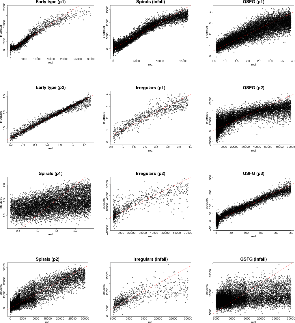 |
Figure 13: Galaxy parameter estimation performance. For each of the input APs we plot the predicted vs. true AP values for the test set. The red line indicates the line of perfect estimation. The summary errors are given in Table 7. |
| Open with DEXTER | |
Table 7: Summary of the performance of the SVM regression models for predicting the input APs of the galaxy models.
range of the input parameters used for them is very different. In particular, the values of the infall timescale are much higher in the case of starbust and irregular galaxies, especially compared to their age (see Table 2). This leads to degeneracies in the produced spectra. For example, galaxies that include a significant gas component and are dominated by a young stellar population might have the same amount of gas as galaxies with older stellar populations that are expected to have depleted their gas component, but may have ongoing gas infall. For the case of the current SFR, we observe that for many galaxies with a zero SFR, the estimated value was quite high. This is mainly a problem caused by the quenched star-forming galaxies for which the SFR is currently zero but in many cases the SF stopped only very recently (e.g., 1 Myr ago). This scenario would lead to a spectrum that is very similar to that of an irregular galaxy (i.e., with a high current SFR) and it is therefore difficult for the SVMs to identify.
For all the other parameters, the results are very accurate. These
results indicate that we will be able to predict most of the
astrophysical parameters that characterize the galaxy spectra with
quite good accuracy, at least for ![]() .
.
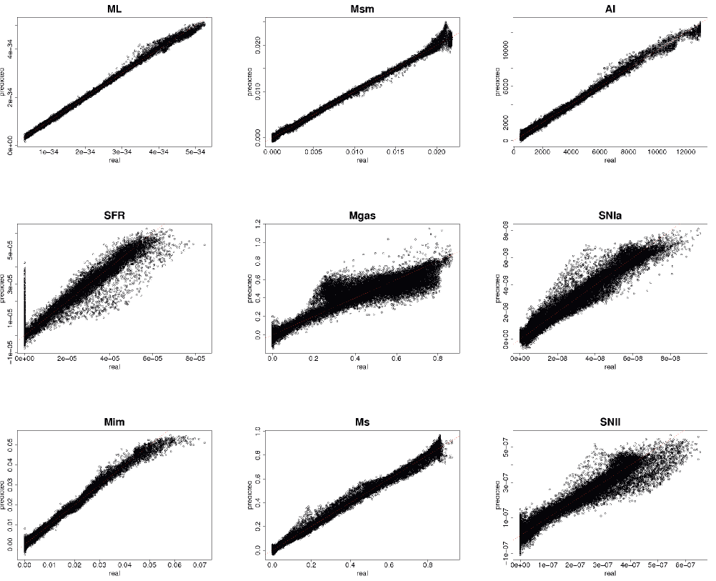 |
Figure 14: Galaxy parameter estimation performance. For each of the output APs we plot the predicted vs. true AP values for the test set. The red line indicates the line of perfect estimation. The summary errors are given in Table 8. |
| Open with DEXTER | |
Table 8: Similar to Table 7 but for the prediction of the output APs of the galaxy models.
7.2 Galaxies with redshift, without reddening at G = 18.5
We present both the classifications of galaxy type and the regressions of redshift for 144 425 simulated spectra of random redshift, without reddening at G=18.5. In both cases, 14 440 spectra were used for training and 129 985 for testing. Only a coarse search for the optimal SVM hyperparameters was performed.
In Tables 9 and 10 (confusion matrices), we can see that the misclassifications numbered 454 for the training and 6813 for the testing set correspond to errors of 3.1% and 5.2% respectively. Comparing the results with those in Sect. 7.1.1 (2.9% for the testing set), we can see that although the error is small it is still two times larger. This result agrees with those in our previous paper (Tsalmantza et al. 2007) for the tests of the first library, where we concluded that the redshift is a parameter that should be estimated in advance of the classification and the estimation of the other parameters.
If we follow this classification scheme, the accuracy in the performance of regression for the redshift parameter will be very important to all the results we will extract from galaxy observations with Gaia. Using the same subsets for training and testing SVMs and following the same procedure for tuning as in the classification we extracted the values of redshift. The results are very good and they are presented in Table 11 and Fig. 15. This is very promising for the performance of the classification and parametrization of the Gaia galaxy observations.
7.3 Galaxies with reddening, redshift at G = 18.5
We used the 144 425 galaxy spectra that include the effects of reddening to perform a regression analysis of theAs expected, the results of the regression analysis for the redshift parameter (Fig. 16 and Table 12) are worse than in the case where no reddening was included in the data, the problem becoming increasingly obvious towards high redshift. This indicates that we should estimate the reddening values before performing the regression of the redshift.
The results of regression for the ![]() parameter are once again very
good (Fig. 17 and Table 12). These results are promising,
because they indicate that we should be able to
estimate the effects of extinction with reasonable
accuracy before extracting the values of the redshift and performing
the rest of our classification scheme. We plan to compare the
parameter are once again very
good (Fig. 17 and Table 12). These results are promising,
because they indicate that we should be able to
estimate the effects of extinction with reasonable
accuracy before extracting the values of the redshift and performing
the rest of our classification scheme. We plan to compare the ![]() estimated in this way with that estimated from Gaia data of nearby
stars.
estimated in this way with that estimated from Gaia data of nearby
stars.
8 Discussion and conclusion
The first results of the SVM classification and parametrization of the second library of synthetic galaxy spectra are very good for the classification of galaxy types and regression of most of the output parameters of the model, redshift, and reddening. However, we emphasize that although the regression results seem to be quite accurate for most output parameters estimated here (e.g., current SFR, metallicity, stellar mass), they might include large errors because of discrepancies between models and reality. All the parameter values used here to train the SVM classifiers are model dependent. The models used are a simplification of the complex structure and evolution of galaxies and therefore cannot lead to accurate predictions of their parameters. These models also are unable to simulate the complete range of detail occuring in the universe. For these reasons, the results presented here should be used for statistical studies of the main galaxy properties in the local universe and not as absolute values for each individual galaxy. In contrast to the output parameters, the results are very poor for the majority of the astrophysical parameters used to produce each type of galaxy, implying that Gaia will not be able to provide accurate measurements for input galaxy parameters. However, this is something that we should investigate further (i.e., using different parametrization methods) to check whether these results can be improved.
Table 9: Galaxy classification with the SVM for the training set.
Table 10: As Table 9 but for the test set.
Table 11: Summary of the performance of the SVM regression models for predicting the z.
We have used the PÉGASE.2 galaxy evolution model and observational data from SDSS to solve problems with our first library and extend the library to cover the large majority of observational data parameter space. In this way, an extended library of 28 885 synthetic galaxy spectra was created at zero redshift and reproduced in addition for 4 random values of redshift. The whole library was produced for a random grid of the astrophysical parameters used by PÉGASE.2 models. The models used in PÉGASE.2 to create early-type galaxies was changed and an exponential model for their SFR was adopted. Models for quenched star-forming galaxies which were not included in the first library were also added. In the case of irregular and spiral galaxies we extended the range of input parameter values. The resulting library includes four general Hubble types instead of seven that were included in the first library and covers almost all the variance in the SDSS photometric observations. To investigate the range of input parameters in the models for each type we made use of photometric data (SDSS and Paturel et al. 1997). Even though the comparison of our library with colour observations provides good results, it is possible that some combinations or values of input parameters produce spectra that do not correspond to realistic galaxy spectra of those types. As an example, we propose that values of the p1 parameter of the early-type galaxies as high as 30 Gyr might lead to unrealistic spectra of early-type galaxies. These values were kept because of the good agreement with the photometric observations but they might be excluded or characterized as spectra of a different galaxy type in future versions of our library if they are found not to match real spectra. For this purpose, we intend to compare the second library of synthetic spectra of galaxies with a larger sample of observational spectra from SDSS.
![\begin{figure}
\par\includegraphics[angle=-90,width=9cm]{12014034.ps}
\end{figure}](/articles/aa/full_html/2009/36/aa12014-09/img33.png) |
Figure 15: Galaxy redshift estimation performance. We plot the predicted versus true z values for the test set. The red line indicates the line of perfect estimation. The summary errors are given in Table 11. |
| Open with DEXTER | |
The second library produced here was compared with other observations, both photometric (Paturel et al. 1997) and spectroscopic (Kennicutt 1992), and found to be in good agreement with them. The only problem appears in the case of quenched star-forming galaxies where the synthetic spectra of this type do not seem to fit very well any type of observed spectra in the Kennicutt Atlas (Fig. A.5). Additionally, even though the SDSS colours of this type of galaxy are very similar to those of starburst galaxies, the comparison of the spectra of these two types showed that they do not reproduce the strong emission lines present in the observational data. To solve this problem we intend to produce starburst galaxies using a new version of the PÉGASE model that includes new models for all the mechanisms that are important to this type of galaxy. In future versions of our synthetic library, we intend to investigate the role of a wider range of astrophysical parameters in the models used in PÉGASE. For example, we need to investigate the range of galaxy age parameter, which has a great impact on the output spectra. Here, it was simply kept constant at 9 or 13 Gyr depending on the galaxy type.
Table 12:
As table 11 for the z and ![]() parameters
for galaxy spectra that include redshift and reddening.
parameters
for galaxy spectra that include redshift and reddening.
![\begin{figure}
\par\includegraphics[angle=-90,width=9cm]{12014035.ps}
\end{figure}](/articles/aa/full_html/2009/36/aa12014-09/img34.png) |
Figure 16: Galaxy redshift estimation performance. We plot the predicted versus true z values for the test set. The red line indicates the line of perfect estimation. The summary errors are given in Table 12. |
| Open with DEXTER | |
For the task of classification and parametrization of unresolved galaxies with Gaia, we will also construct a semi-empirical library of galaxy spectra. This library will include observational spectra from SDSS, which will be extended to the wavelength range of Gaia by our synthetic spectra. The advantage of this library is that it provides a set of real observed spectra, with the corresponding astrophysical parameters, as defined by comparing each spectrum with the synthetic spectra. A library of observed galaxy spectra combined with the already produced synthetic libraries will check and improve our classification system and test the reliability and completeness of our libraries.
![\begin{figure}
\par\includegraphics[angle=-90,width=9cm]{12014036.ps}
\end{figure}](/articles/aa/full_html/2009/36/aa12014-09/img35.png) |
Figure 17:
Galactic-interstellar extinction estimation performance. We plot
the predicted versus true |
| Open with DEXTER | |
Acknowledgements
The authors would like to thank the Greek General Secretariat of Research and Technology (GSRT) for financial support and the ELKE of UOA. P. Tsalmantza would also like to thank the Institut d'Astrophysique de Paris (IAP) for their support and hospitality.
This work makes use of Gaia simulated observations and we thank the members of the Gaia DPAC Coordination Unit 2, in particular Paola Sartoretti and Yago Isasi, for their work. These data simulations were done with the MareNostrum supercomputer at the Barcelona Supercomputing Center - Centro Nacional de Supercomputacion (The Spanish National Supercomputing Center).
Funding for the Sloan Digital Sky Survey (SDSS) has been provided by the Alfred P. Sloan Foundation, the Participating Institutions, the National Aeronautics and Space Administration, the National Science Foundation, the US Department of Energy, the Japanese Monbukagakusho, and the Max Planck Society. The SDSS Web site is http://www.sdss.org/. The SDSS is managed by the Astrophysical Research Consortium (ARC) for the Participating Institutions. The Participating Institutions are The University of Chicago, Fermilab, the Institute for Advanced Study, the Japan Participation Group, The Johns Hopkins University, the Korean Scientist Group, Los Alamos National Laboratory, the Max-Planck-Institute for Astronomy (MPIA), the Max-Planck-Institute for Astrophysics (MPA), New Mexico State University, University of Pittsburgh, University of Portsmouth, Princeton University, the United States Naval Observatory, and the University of Washington.
Appendix A: Comparison of the second library with Kennicutt's atlas
We present the results of the
| |
Figure A.1:
Results of the |
| Open with DEXTER | |
![\begin{figure}\par\mbox{\includegraphics[angle=-90,width=2.2cm]{12014053.ps}\inc...
...4083.ps}\includegraphics[angle=-90,width=2.2cm]{12014084.ps} }
\par
\end{figure}](/articles/aa/full_html/2009/36/aa12014-09/img37.png) |
Figure A.2: The same with Fig. A.1 for the spiral galaxies in Kennicutt's atlas. first row: NGC 1357, NGC 2276, NGC 2775, and NGC 4775, second row: NGC 5248, NGC 3368, NGC 3623, and NGC 6217, third row: NGC 1832, NGC 2903, NGC 3147, and NGC 4631, fourth row: NGC 3627, NGC 6181, NGC 4750, and NGC 6643. |
| Open with DEXTER | |
| |
Figure A.3: The same with Fig. A.1 for the magelanic type irregular galaxies in Kennicutt's atlas. Here we present: NGC 1569, NGC 4485, NGC 4449, and NGC 4670. |
| Open with DEXTER | |
| |
Figure A.4: The same with Fig. A.1 for the I0 irregular galaxies in Kennicutt's atlas. Here we present: NGC 3034, NGC 5195, NGC 3077, and NGC 6240. |
| Open with DEXTER | |
| |
Figure A.5: The same with Fig. A.1 for the starburst galaxies with global starbursts in Kennicutt's atlas. Here we present: NGC 3310, NGC 6052, NGC 3690, and UGC 6697. |
| Open with DEXTER | |
| |
Figure A.6: The same with Fig. A.1 for the nuclear starburst galaxies in Kennicutt's atlas. Here we present: NGC 2798, NGC 3471, NGC 5996, and NGC 7714. |
| Open with DEXTER | |
References
- Bailer-Jones, C. A. L. 2006, MmSAI, 77, 1144 [NASA ADS] (In the text)
- Bailer-Jones, C. A. L., Smith, K. W., Tiede, C., Sordo, R., & Vallenari, A. 2008, MNRAS, 391, 1838 [NASA ADS] [CrossRef] (In the text)
- Fioc, M. 1997, Ph.D. Thesis (In the text)
- Fioc, M., & Rocca-Volmerange, B. 1997, A&A, 326, 950 [NASA ADS]
- Fioc, M., & Rocca-Volmerange, B. 1999a, A&A, 344, 393 [NASA ADS] (In the text)
- Fioc, M., & Rocca-Volmerange, B. 1999b, A&A, 351, 869 [NASA ADS] (In the text)
- Groenewegen, M. A. T., & de Jong, T. 1993, A&A, 267, 410 [NASA ADS] (In the text)
- Kennicutt, R. C. Jr 1992, ApJS, 79, 255 [NASA ADS] [CrossRef] (In the text)
- Le Borgne, D., & Rocca-Volmerange, B. 2002, A&A, 386, 446 [NASA ADS] [CrossRef] [EDP Sciences] (In the text)
- Paturel, G., Andernach, H., Bottinelli, L., et al. 1997, A&AS, 124, 109 [NASA ADS] [CrossRef] [EDP Sciences] (In the text)
- Perryman, M. A. C., de Boer, K. S., Gilmore, G., et al. 2001, A&A, 369, 339 [NASA ADS] [CrossRef] [EDP Sciences] (In the text)
- Rana, N., & Basu, S. 1992, A&A, 265, 499 [NASA ADS] (In the text)
- Tsalmantza, P., Kontizas, M., Bailer-Jones, C. A. L., et al. 2007, A&A, 470, 761 [NASA ADS] [CrossRef] [EDP Sciences] (Paper I) (In the text)
- Turon, C., O' Flaherty, K. S., & Perryman, M. A. C. 2005, ESASP, 576 (In the text)
- Yi Sukyoung, K. 2003, ApJ, 582, 202 [NASA ADS] [CrossRef] (In the text)
Footnotes
All Tables
Table 1: Models of SF assumed in the new library.
Table 2: Input parameters for the galaxy scenarios in the new library.
Table 3: Classification results for galaxy spectra in the Kennicutt's atlas.
Table 4: The number of spectra and the tuning scheme used for the various SVM tests.
Table 5: Galaxy classification with the SVM for the training set.
Table 6: As Table 5 but for the test set.
Table 7: Summary of the performance of the SVM regression models for predicting the input APs of the galaxy models.
Table 8: Similar to Table 7 but for the prediction of the output APs of the galaxy models.
Table 9: Galaxy classification with the SVM for the training set.
Table 10: As Table 9 but for the test set.
Table 11: Summary of the performance of the SVM regression models for predicting the z.
Table 12:
As table 11 for the z and ![]() parameters
for galaxy spectra that include redshift and reddening.
parameters
for galaxy spectra that include redshift and reddening.
All Figures
| |
Figure 1: The first library of synthetic galaxy spectra. The SDSS galaxies, the galaxies produced in the first library, and the typical synthetic spectra of PÉGASE.2 are presented with black, red, and yellow dots, respectively. |
| Open with DEXTER | |
| In the text | |
| |
Figure 2: Models of Im galaxies with SFR stopping at 1 Myr to 2 Gyr ago (magenta). Black dots are the SDSS galaxies and red the 8 typical synthetic spectra of PÉGASE.2. |
| Open with DEXTER | |
| In the text | |
| |
Figure 3: Models of E galaxies produced assuming exponential star formation rate (magenta). Black dots are SDSS galaxies and red the 8 typical synthetic spectra of PÉGASE.2. |
| Open with DEXTER | |
| In the text | |
| |
Figure 4: Models of irregular (blue), quenched star-forming galaxies (magenta), spirals (light blue), and early-type galaxies (red). Black dots are SDSS galaxies and green the 8 typical synthetic spectra of PÉGASE.2. |
| Open with DEXTER | |
| In the text | |
| |
Figure 5: Early-type, spiral, and irregular (red, green, and blue) galaxies derived from the LEDA catalog. Black dots are all galaxies (including quenched star-forming galaxies) produced by PÉGASE.2. |
| Open with DEXTER | |
| In the text | |
| |
Figure 6: As in Fig. 5, but now the black dots are the properties of irregular galaxies produced by PÉGASE.2. |
| Open with DEXTER | |
| In the text | |
| |
Figure 7: As in Fig. 5, but now the black dots are the properties of spiral galaxies produced by PÉGASE.2. |
| Open with DEXTER | |
| In the text | |
| |
Figure 8: As in Fig. 5, but now the black dots are the properties of early-type galaxies produced by PÉGASE.2 |
| Open with DEXTER | |
| In the text | |
| |
Figure 9: Distribution (normalized) of B-V colours for early-type, spiral, and irregular (red, black, and blue respectively) galaxies derived from the LEDA catalog. |
| Open with DEXTER | |
| In the text | |
| |
Figure 10: Distribution (normalized) of B-V colours for early-type, spiral, irregular and quenched star-forming (red, black, blue and green respectively) galaxies produced by PÉGASE.2 code. |
| Open with DEXTER | |
| In the text | |
| |
Figure 11: Random models of irregular (blue), quenched star-forming galaxies (magenta), spirals (light blue), and early-type galaxies (red). Black dots are SDSS galaxies and green the 8 typical synthetic spectra of PÉGASE.2. |
| Open with DEXTER | |
| In the text | |
| |
Figure 12:
The mean S/N spectrum of the simulated galaxy spectra used
in the classification tests. Only points with
|
| Open with DEXTER | |
| In the text | |
| |
Figure 13: Galaxy parameter estimation performance. For each of the input APs we plot the predicted vs. true AP values for the test set. The red line indicates the line of perfect estimation. The summary errors are given in Table 7. |
| Open with DEXTER | |
| In the text | |
| |
Figure 14: Galaxy parameter estimation performance. For each of the output APs we plot the predicted vs. true AP values for the test set. The red line indicates the line of perfect estimation. The summary errors are given in Table 8. |
| Open with DEXTER | |
| In the text | |
| |
Figure 15: Galaxy redshift estimation performance. We plot the predicted versus true z values for the test set. The red line indicates the line of perfect estimation. The summary errors are given in Table 11. |
| Open with DEXTER | |
| In the text | |
| |
Figure 16: Galaxy redshift estimation performance. We plot the predicted versus true z values for the test set. The red line indicates the line of perfect estimation. The summary errors are given in Table 12. |
| Open with DEXTER | |
| In the text | |
| |
Figure 17:
Galactic-interstellar extinction estimation performance. We plot
the predicted versus true |
| Open with DEXTER | |
| In the text | |
| |
Figure A.1:
Results of the |
| Open with DEXTER | |
| In the text | |
| |
Figure A.2: The same with Fig. A.1 for the spiral galaxies in Kennicutt's atlas. first row: NGC 1357, NGC 2276, NGC 2775, and NGC 4775, second row: NGC 5248, NGC 3368, NGC 3623, and NGC 6217, third row: NGC 1832, NGC 2903, NGC 3147, and NGC 4631, fourth row: NGC 3627, NGC 6181, NGC 4750, and NGC 6643. |
| Open with DEXTER | |
| In the text | |
| |
Figure A.3: The same with Fig. A.1 for the magelanic type irregular galaxies in Kennicutt's atlas. Here we present: NGC 1569, NGC 4485, NGC 4449, and NGC 4670. |
| Open with DEXTER | |
| In the text | |
| |
Figure A.4: The same with Fig. A.1 for the I0 irregular galaxies in Kennicutt's atlas. Here we present: NGC 3034, NGC 5195, NGC 3077, and NGC 6240. |
| Open with DEXTER | |
| In the text | |
| |
Figure A.5: The same with Fig. A.1 for the starburst galaxies with global starbursts in Kennicutt's atlas. Here we present: NGC 3310, NGC 6052, NGC 3690, and UGC 6697. |
| Open with DEXTER | |
| In the text | |
| |
Figure A.6: The same with Fig. A.1 for the nuclear starburst galaxies in Kennicutt's atlas. Here we present: NGC 2798, NGC 3471, NGC 5996, and NGC 7714. |
| Open with DEXTER | |
| In the text | |
Copyright ESO 2009
Current usage metrics show cumulative count of Article Views (full-text article views including HTML views, PDF and ePub downloads, according to the available data) and Abstracts Views on Vision4Press platform.
Data correspond to usage on the plateform after 2015. The current usage metrics is available 48-96 hours after online publication and is updated daily on week days.
Initial download of the metrics may take a while.