---

Modelling of solar mesogranulation

. Matloch - R. Cameron - D. Schmitt - M. Schüssler

Max-Planck-Institut für Sonnensystemforschung, Max-Planck-Strasse 2, 37191 Katlenburg-Lindau, Germany

Received 21 October 2008 / Accepted 5 June 2009

Abstract
We study whether mesogranulation flow patterns at the solar surface can arise solely from the statistical properties of granules and intergranular lanes. We have developed one- and two-dimensional models with local interaction rules between the artificial ``granules'' mimicking the actual physical processes on the solar surface. Defining mesogranulation according to the age of intergranular (downflow) lanes corresponding to the often applied ``cork method'', as well as the areas of divergence of the horizontal velocity (two-dimensional model), we find that mesogranular patterns are present in our models. Our study of the dependence of the properties of the mesogranular patterns on the model parameter and interaction rules reveals that the patterns do not possess intrinsic length and time scales.

Key words: Sun: granulation

1 Introduction

The phenomenon of mesogranulation, an apparent flow pattern with spatial scales of about 4-10 Mm and time scales of a few hours, has eluded any convincing physical explanation since its discovery (November et al. 1981). Mesogranular patterns appear in divergence maps of horizontal flows inferred by local correlation tracking of tracers, such as granules and magnetic flux concentration (November 1989; Muller et al. 1992; Roudier et al. 1998; Shine et al. 2000). Associated intensity variations on the same scales have not been found. Proposals for the origin of mesogranulation include a distinct convective scale, a spatial and temporal arrangement of exploding granules, or an artifact of data analysis. Even though evidence for a clearly defined ``mesoscale'' is weak (Wang 1989; Chou et al. 1991; Rast 1991; Strauss et al. 1992; Rast & Toomre 1993; Strauss & Bonaccini 1997; Rieutord et al. 2000; Georgobiani et al. 2007), the existence of horizontal flows on scales between granulation and supergranulation is supported by both observations and hydrodynamical simulations. The possibility that mesogranulation results from convective driving at the depth of the first helium ionization around 7 Mm has been ruled out by the appearance of the mesoscale patterns in ``shallow'' numerical simulation that do not reach this depth (Ploner et al. 2000) or do not include ionization effects at all (Cattaneo et al. 2001).

Near-surface mesoscale flows without a characteristic scale may reflect the flow topology suggested by Stein & Nordlund (1989) on the basis of numerical simulations: merging downflows lead to a gradual increase of horizontal scale of the convective upflows and horizontal flows with depth, such that smaller-scale patterns are advected by those on larger scales. Another (not necessarily completely unrelated) approach is to study specific properties of granules in relation to mesogranular patterns. For instance, the effects of exploding or fragmenting granules, which expand rapidly, have been considered. The average granule lifetime is about ten minutes and the diameter of an exploder rarely exceeds 2 Mm, hence individual exploding granules cannot sustain the mesogranular pattern. Nevertheless, a sequence of neighbouring exploder events could in principle last long enough to produce a larger coherent velocity structure. Oda (1984) studied the surface distribution of fragmenting granules and suggested that they outline a mesoscale pattern, while Hirzberger et al. (1997) found that fragmenters exist predominantly in the mesogranule centres. Simon et al. (1991) showed that a simple kinematic model of exploder events that are normally distributed around a centre of a would-be mesogranule can reproduce patterns similar to those found in observational studies. On the other hand, a fully random distribution of exploders does not produce any coherent patterns in their model. The question whether exploders are organised on the solar surface was also explored by Rieutord et al. (2000) and Roudier et al. (2003, 2004). They analysed recurrently fragmenting granules (``trees of fragmenting granules'', TFGs) and found that TFGs cover over of the solar surface at any given time. The lifetime of such granule families can reach many hours, but the distribution indicates no characteristic time scale. The velocity field produced by a TFG, when averaged over the its lifetime, yields a velocity divergence (outflow) area, with many of the TFGs reaching an area of 6 Mm diameter. These features of the TFGs bear resemblance to mesogranules. This suggests that mesogranulation might be related to the properties and the spatial and temporal arrangement of granules.

Rast (2003) proposed an alternative model in which larger-scale patterns emerge from the interaction of thermal downflows on the solar surface. In his model, the downflow plumes are generated at random locations and evolve through mutual advection, which leads to plume merging and results in strong downflows being distributed with a characteristic length scale. Such strong long-lived downflows then define the vertices of the mesogranular or supergranular cells, while the associated large-scale horizontal flows result from mass conservation. Another approach to pattern formation by self-arrangement has been suggested by Crouch et al. (2007) in connection with the origin of the supergranular magnetic network. These authors consider a random advection of accumulating and cancelling small scale magnetic elements on the solar surface and conclude that such process can lead to the emergence of larger-scale patterns.

The models presented in this work explore the idea that mesogranular patterns can arise from the interaction of granules. This work is split into two parts: in the first part we present a one-dimensional model, which introduces the concept of parameterizing granulation as a cell system. The time-slice diagrams of solar granulation (one spatial dimension versus time) indicate a characteristic tree-like pattern of intergranular lanes (Müller et al. 2001), which is also shown by numerical simulation (Ploner et al. 1998, 1999, 2000). Such a system can easily be reproduced by the artificial granulation model presented in this work, where the granules are identified as spaces separating the intergranular lanes. Merging of the lanes marks the disappearance of a granule and an appearance of a new intergranular lane marks the splitting of a granule. The advantage of this model is its simplicity which permits us to study various interaction schemes and a large range of parameters. We show that the model represents the spatially one-dimensional granulation in observational time-slice diagrams and in two-dimensional numerical simulations quite well. We analyse the properties of the structures at mesogranular sizes and show that these emerge naturally in such cell systems. We investigate how the granule evolution rules affect the results, including also a random-walk version of the granulation model.

In the second part we describe a two-dimensional extension of the model, with the granules arranged horizontally on a plane. We apply various granule evolution rules and different analysis methods to investigate the properties of the mesoscale structures. In particular, in the two-dimensional model we can apply the same methods as used in the analysis of observations and numerical simulations, which allows for a direct comparison of the results. By studying the effects of different granule interaction rules on the properties of the emerging mesogranulation, we are able to identify the processes that lead to the appearance of the mesogranular pattern.

2 Interaction and splitting of granules

The interaction rules in our models are based on the simplification of the physics of evolution of the solar granules. We are mainly interested in the horizontal interaction between neighbouring granules and the fragmentation process. The horizontal interaction can be understood as follows: granules evolve slowly compared with the acoustic timescale, leading to a relation between granule size and the pressure at its boundary. Namely, the larger the granule is, the higher the pressure excess above its centre must be to deflect the rising plasma horizontally and sustain the granular outflow (e.g. Nordlund 1985). This pressure excess is accompanied by corresponding pressure excess at the cell boundary (intergranular lane), which decelerates the outflowing plasma near the downflow lanes (Stein & Nordlund 1998; Ploner et al. 1999). The pressure difference between two granules of different sizes causes the intergranular lanes to move towards the smaller granule. Therefore, large granules tend to spread, pushing the surrounding downflow lanes outwards and squeezing the smaller neighbours.

The mechanism for the splitting of granules is also related to the pressure conditions: when a granule exceeds a critical size of 1 Mm (Hirzberger et al. 1997, 1999), the upflow in the cell centre diminishes. This is caused by a pressure buildup at the top of the cell, which is proportional to the granule size and which deflects the upflowing plasma horizontally. Such pressure also reduces the upward plasma motion, and when the granule exceeds the critical size, the pressure buildup has become large enough to locally stop the plasma upflow. Without the upflow from below, the plasma at the top of the cell cools radiatively until it is dense enough to sink back into the interior, forming a new downflow plume and breaking up the granule. This is called ``buoyancy braking''. An alternative interpretation of the granulation cell pattern evolution in terms of the downflow plumes have been proposed by Rast (1995, 2003): downflowing plumes initiate time-limited upflows in their surroundings. A spatial arrangement of these downflows on the solar surface leads to the formation of the granulation cell pattern, with the upflow in the cell centre being the sum of all the contributions from the response flows initiated by the dowflows surrounding the granule. The critical granule cell size can then be explained as the maximum cell size that given downflows can sustain. When the granule expands, the downflows are pushed apart and hence the response upflow in the cell centre diminishes below that needed to sustain the circulation. The granule interaction and splitting rules in our simplified models are consistent with both interpretations of the observed behaviour of solar granules.

3 One-dimensional model

3.1 Model description

The model has one spatial dimension and traces the evolution of artificial granules in time, hence producing plots of granule positions versus time. The model is quite simple and does not aim at a quantitative reproduction of solar granulation, but rather serves to introduce the concept of describing the evolution of a set of granules as a cell system with simple interacting rules. Such reduction to a rudimentary system allows to study which properties suffice to provide a mesogranular pattern. The model also allows for comparison with two-dimensional hydrodynamic simulations (depth plus one horizontal coordinate) by Ploner et al. (1998, 1999, 2000) and Steiner (2003). The granules are defined as the spaces between the intergranular lanes, which in turn are described by movable points. The points start from an initial distribution and move along the spatial dimension in time, therefore producing lines in a time-distance diagram. Thus, at any given time, there are a number of granules present in the simulation, their sizes being the distances between neighbouring points.

The spatial domain is periodic. We consider a ``cell competition'' model, which means that the movement of any given point (intergranular lane) is determined by the difference of ``pressures'' exerted on it by the two granules that the point separates. In a real flow, it is the fluid parcels that respond to the pressure force. In this simplified model, this is replaced by the resulting effect on the location of the downflow structures. Assuming a linear relation between granule size and pressure we obtain the following rules of intergranular lane movement: let x_i be the spatial position of i-th point, then

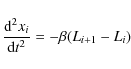
where L_i is the size of the granule defined by the interval [x_i-1,x_i] and is a proportionality constant. Hence, intergranular lanes are points of pressure discontinuity in the model. We have also run models with (acceleration) in Eq. (1) changed to (velocity). The results are qualitatively similar (see also: Rast 1999).

When two points meet they merge, marking the disappearance of a granule. On the other hand, when an expanding granule reaches a critical size, it is assumed to split in two, with a new point (intergranular lane) appearing. In our model the critical size for fragmentation is set to

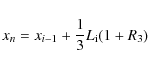
where R₁ is a random number from a uniform distribution in the range [0,1] and R₂ is a normally distributed random number with both variance and standard deviation equal to unity. The random numbers R₁ and R₂are determined individually for each granule at each timestep. We checked different combinations of random numbers and found that the distribution given by Eq. (2) gives the best approximation of the granular distributions of Ploner (1998). The position x_n of the new intergranular lane is chosen randomly within the middle third part of the splitting granule, i.e.,

where R₃ is an uniformly distributed random number in the range [0,1]. Lanes can appear, but not disappear other than by lane merging (dissolving granule). Figure 1 presents an example of a granule evolution plot, i.e. a time-distance diagram. The lines represent intergranular lanes, which evolve with time from left to right. The appearance of a new lane marks the splitting granule (fragmenter), while lane merging marks the disappearance of a granule (dissolver).

3.2 Granule properties

The arbitrary time scale of the model is fixed by the requirement that the mean granule lifetime agrees with the value of 8.2 min in the hydrodynamical simulation of Ploner et al. (1999), which also has one spatial dimension. We now compare the results of our model with further properties of the results of Ploner et al. (1998, 1999) and those observed by Müller et al. (2001). We present statistics for two kind of cells: dissolvers (granules that eventually disappear by being squeezed out by their neighbours) and fragmenters (granules that finally split into offspring granules). Figure 2a shows lifetime histograms of dissolvers and fragmenters from a simulation similar to that of Fig. 1, but run in a larger domain (  h) to include more granules. Figure 2b shows the size distributions of dissolvers and fragmenters, with mean values  Mm and  Mm, respectively. While the distribution of lifetimes is very similar for dissolvers and fragmenters, their sizes (average over lifetime) differ significantly. This is further illustrated in Fig. 2c, which gives a scatter plot of granule lifetime versus size. The cells with the shortest lifetimes in the cellular model are the smallest dissolvers and the largest fragmenters. This is not surprising: the smaller the initial size of a dissolver, the faster it is squeezed out of existence by its neighbours. The large fragmenters exceed the critical splitting size soon after they appear, hence their short lifetime. From Fig. 2 it is clear that there is little overlapping of average granule sizes between dissolvers and fragmenters. Nevertheless, the long-lived granules approach the mean size regardless of the way they disappear. The distributions obtained by Ploner et al. (1998, 1999) show similar separation of sizes between dissolvers and fragmenters, with the longest-lived cells approaching the mean granule size.

Table 1:   Granule characteristics.

Table 1 summarises the averaged granular parameters derived from the model; the global mean lifetime (``diss + frag'') has been scaled such that it agrees with the value obtained by Ploner et al. (1998, 2000). Although the model is very simple, it reproduces rather well the statistical properties of the simulated one-dimensional granules (Ploner et al. 1998, 1999) and observed time-slice diagrams (Müller et al. 2001), with the lifetimes being almost the same for both cell types, and a separation of the sizes. This indicates that the basic mechanism for granule interaction is described reasonably well by our simplified cell system.

3.3 Mesogranulation

3.3.1 Definition

One way to detect mesogranulation in observational data is by means of ``corks'', artificial test particles which are passively advected by the horizontal flow as determined by local correlation tracking of intensity features (Simon & Weiss 1989; Shine et al. 2000; Leitzinger et al. 2005). The corks tend to gather in the long-lived intergranular downflow lanes, which represent places of horizontal velocity convergence. The resulting patterns have lifetimes exceeding the average granule lifetime and outline areas of horizontal fluid divergence which are identified as mesogranules (Simon et al. 1991; Ploner et al. 2000; Rieutord et al. 2000; Roudier et al. 2003; Cattaneo et al. 2001).

Averaging the horizontal velocity over time can indeed show flow structures with a mean radial outflow from the centre of a mesocell, although the instantaneous velocities are strongly fluctuating (Rieutord et al. 2000). In our model, there are no explicit fluid motions, but we can define a mesogranular downflow lane as an intergranular lane that exceeds a certain minimum lifetime (and thus would accumulate a large number of corks). Accordingly, we mark intergranular lanes that have lifetime longer than a given threshold, t₀, as mesogranular. Whenever two lanes merge, we keep the lifetime of the older one. Figure 3 shows a similar granule evolution as Fig. 1, now with the mesogranular lanes marked thick for t₀=50 min.

3.3.2 Properties

Similar to granules, we can divide mesogranules into meso-fragmenters and meso-dissolvers, according to the modes of their decay. Figures 4a and 4b give the lifetime and size distribution, respectively, of mesogranules from the model run shown in Fig. 3, (run in a larger domain of  h to include more mesogranules). Figure 4c is a scatter plot of mesogranular lifetime versus size. Table 2 contains a summary of averaged mesogranular characteristics for threshold time t₀=50 min. Comparing Figs. 2 and 4 indicates that mesogranulation defined in this manner bears a striking similarity to granulation, although the model contains no explicit rules for its evolution. Just like in case of granules, the lifetime distributions for the two types of mesogranules are very similar, while there is a clear separation of their sizes. Moreover, the mesogranules approach the mean size with increasing lifetime, regardless of whether they are mesodissolvers or mesoexploders, just like the granules do. Since the mode of decay does not depend on the history of a granule or mesogranule, it has little effect on the mean size for long-lived structures. The mean size is such that a (meso)granule can survive for a long time because it is neither probable that it splits, nor does it face being squeezed by its neighbours.

Table 2:   Mesogranule characteristics, t₀=50 min.

In Fig. 4c there is a separation of meso-fragmenters and meso-dissolvers similar to that of Fig. 2c for granules, and similar arguments can be employed to explain it. Like granules, the mesogranules in the model are born through fragmentation of the parent object. The splitting mechanism is not explicitly built into the mesogranule evolution, but rather follows from the evolution of granules. The fact that in Fig. 4c the largest meso-fragmenters have the shortest lifetimes can be explained as follows: if a mesogranule is large, it contains a large number of intergranular lanes. Therefore, there is a higher probability that one of them exceeds the lifetime limit in the next timestep and becomes a mesogranular lane, thus splitting the original mesogranule.

3.3.3 Dependence on threshold time

In order to study the dependence of the mesogranule properties on the threshold time t₀, it is instructive to consider the behaviour of the oldest intergranular lanes in the simulation, i.e. lanes that start at t=0(called zero lanes in what follows). Their number decreases in time by merging of such lanes in which case we keep the age of the older one. Figure 5 shows the number of zero lanes versus time. The decrease of the number of zero-lanes is consistent with the function N(t)=At^-1/2 (dashed line). Such behaviour is expected from zero-lanes performing a random walk in the domain (e.g, Chandrasekhar 1943). We conclude that even though the granules evolve according to the cell-competition rules, the long-term cumulative effect of such rules on a particular lane is equivalent to the lane performing a random walk.

The behaviour of the zero lanes also indicates that the mean properties of the mesogranules should depend on the threshold time, t₀. Because there is nothing special about t=0, the number of lanes which have lived for more than minutes at any time is (statistically) the same as the number of lanes remaining after minutes from time t=0. Thus, Fig. 5 can be interpreted as showing the average number of mesolanes versus the threshold time t₀. When t₀increases, the number of the lanes that are older than t₀ decreases according to the t₀^-1/2 law, which leads to a corresponding increase of the mean mesogranule size and lifetime. This also holds in the statistically stationary state. Figure 6 shows the dependence of the average mesogranular lifetime and size on t₀ in the range between 15 min and 4 h.

The larger t₀ is, the fewer intergranular lanes have reached this value and are present in the domain at a given moment, resulting in a larger size of mesogranules. When the distance between the mesolanes is larger, it takes longer for them to meet and merge, hence the lifetime increases. Similarly, if the t₀ is large, it takes longer for an intergranular lane within a mesogranule to become a mesolane and thus split the existing mesogranule. As a result, mesogranulation as defined by a lifetime threshold of intergranular lanes in the model has no intrinsic time- and length-scales, since these values depend on the choice of the threshold time t₀.

3.4 A random-walk model

In order to study how strongly the granule interaction rules affect the mesogranular properties, we consider a random-walk model, for which the previous rule for lane movement given by Eq. (1) is replaced by a random displacement (with normal distribution). To keep the time scale comparable with the cell-competition model the motion of the lanes has to be faster by a factor of three since the random displacements change the direction of motion much more frequently. Figure 7 shows an example of a granule evolution plot for the random model. Figure 8 gives the corresponding statistics of mesogranules for a threshold time t₀=50 min in the random-walk model, which can be compared to Fig. 4 for the cell-competition model. Clearly, the properties of mesogranulation in the random-walk model are rather similar to that of the cell-competition case. Figure 9 shows that the decay of the number of the zero-lanes in the random-walk model follows the t^-1/2 law. Consequently, the difference between the two models lies predominantly in the short timescale interaction, while the resulting average motion of the intergranular lanes in the cell-competition and the random-walk cases is similar.

Figure 10 shows the dependence of the mean mesogranule size and lifetime on the threshold time t₀ for the random-walk model. The increase of the mean mesogranule size with t₀ (Fig. 10b) can be well approximated with a t₀^1/2 law (dotted line), which is consistent with the t^-1/2 decrease of the number of zero-lanes. The dependence of the mean mesogranule size on threshold time t₀ in the cell-competition model (Fig. 6b) does not fit well the t₀^1/2 law, although the zero-lane decay for that model (Fig. 5) is also consistent with the t^-1/2. This is probably due to the fact that Fig. 6b comprises only threshold times of up to 250 min, covering only a small part of the time span covered by Fig. 5. For such relatively short threshold times, the mesogranules are small enough to still be considerably influenced by the granule interaction rules of the cell-competition model. We expect that the dependence of the mesogranule areas on the threshold time in Fig. 6b asymptotically reaches the t₀^1/2 behaviour for large threshold times.

Figure 10 a shows that the mean mesogranule lifetime is roughly equal to the threshold time, t₀. This relationship can be made plausible as follows. Consider a time interval of length t₀ in the statistically stationary state of the model, so that the number of mesogranules can be assumed to be equal at the beginning and at the end of the interval. From the t₀^-1/2 law for the number of the zero-lanes it follows that about of the mesogranular lanes vanish during this time interval by merging with other mesogranular lanes. This is equivalent to the decay of of the mesogranules as dissolvers. In a stationary state, this means that new mesolanes appear, so that a further of the initially existing mesogranules decay by splitting. In total, there is a chance for the mesogranules that were present at time t to survive until time t+t₀. Consequently, the average lifetime of the mesogranules is of the order of t₀.

In the cell-competition model the dependence of the mean mesogranule lifetime on t₀ (Fig. 6a) deviates from the linear relationship for short threshold times. Nevertheless, for threshold time larger than about two hours we see the linear, almost one-to-one relation similar to the random-walk case. The above explanation of the lifetime behaviour of the mesogranules in the random-walk model in principle also holds for the cell-competition case. The cell-competition granule interaction rules affect only the short times, because the decay of the zero-lanes is similar for both models (cf. Figs. 5 and 9).

3.5 Summary: one-dimensional results

The main conclusion from the one-dimensional model is that the time evolution and basic statistics of the granulation pattern can be reasonably well described by a cell system with simple rules for cell interaction, splitting and decay. Larger-scale patterns, in various ways similar to the one-dimensional mesogranulation detected in numerical models, appear when considering intergranular lanes that exceed a given threshold age. The appearance of such patterns is a robust property of the model; its properties only weakly depend on the detailed granule interaction schemes. The differences between the random walk and the cell-competition cases are largely restricted to the small scales while the resulting statistical properties of mesogranules are quite similar for the two models. On the other hand, the developing mesogranulation has no intrinsic spatial and temporal scales: average size and lifetime depend on the threshold age for the intergranular lanes. The dependence of the mesogranular size and lifetime on the threshold time is similar for the two versions of the model, strengthening the conclusion that there is no characteristic scale associated with the phenomenon. Nevertheless, the model is too simple to draw definite conclusions about the three-dimensional phenomenon on the Sun. Even if the granular arrangement and mesogranulation emergence is largely a surface effect, it still requires at least two dimensions to describe it properly. In the following section we present a two-dimensional extension of the granulation model.

4 Two-dimensional model

4.1 Model description

In the extension of our model to two spatial dimensions we consider the granules as two-dimensional triangular cells. Although higher polygons (such as hexagons) might provide a better representation of solar granules, we have chosen triangles because then we can maintain the topological structure after splitting in a simple way. Splitting other polygons would invariably lead to lower polygons and/or hanging nodes (free vertices). The cell evolution is determined by the motion of the vertices, which translate on the plane according to a given set of rules. The splitting and vanishing of triangular cells is more complicated than in the case of only one spatial dimension. For example, to keep the triangular cell structure, the splitting procedure has to affect two adjacent cells simultaneously. Also, since one method of mesogranulation detection involves the age of the structures, the age inheritance rules when splitting and removing cells have to be set properly. We start with a square grid of d² points which constitute the vertices of triangular cells. Each initial vertex position has a random component to avoid artificial pattern formation and shorten the initial transient phase of the model.

We have considered various model versions in order to study how different evolution rules influence the results. The versions differ mainly by the vertex motion schemes (random-walk and cell-competition) and the granule splitting rules. We will confine the discussion to one cell-competition (C) and one random-walk (R) model. The details of the model construction and the differences between the model versions are given in the Appendix. Sections 4.2 and 4.3 refer to the C model, which aims at an approximation of the properties of solar granulation. In short, the cell-competition rules simulate solar granules in the way that large cells tend to grow in time and squeeze the smaller cells out, splitting once they exceed a critical area, corresponding to the physical arguments given in Sect. 2. The squeezing of small cells and growth of the large ones is achieved by the rule that the vertex of the triangular cell moves in time towards its closest neighbouring vertex. Once a cell exceeds a critical area, it splits, with a new vertex appearing. The random model R, where the evolution of the cell does not depend strongly on the cells' properties, is addressed in Sect. 4.4.

4.2 Granule properties

In this section we consider the distributions of granulation cell sizes and lifetimes for the C model. The lifetime of a cell is the time from its birth by parent-cell splitting to its demise (either by splitting or by vanishing). All times are given in units of the average granule lifetime, which can be scaled to any required value by fixing the free time unit in the model. The size of a cell is taken as the average size over the cell's lifetime. We present statistics for two kinds of cells, distinguished by the way they disappear in the simulation: dissolvers (those who vanish by vertex merging) and fragmenters (those that split). Figure 11 shows the lifetime distribution (a), size distribution (b), a scatter plot of the cell size versus lifetime (c) and a snapshot of the emerging pattern of the triangular granulation for the C model. Similar to the one-dimensional model results, there is a difference of the size distribution between the dissolving and fragmenting granules. Such a difference is known to exist both in numerical simulations and in observational data (Ploner et al. 1998, 1999; Müller et al. 2001). The reported size and lifetime histograms of solar granules depend on the analysis method applied, and vary from one author to another. Nevertheless, most of the observed lifetime histograms are close to exponential, while the area distributions show a monotonic increase of the number of small granules, terminated by the cutoff resulting from limited resolution (Title et al. 1989; Brandt et al. 1991; Hirzberger et al. 1997, 1999; Müller et al. 2001). In contrast to that, in Fig. 11a and 11b the distributions tend to peak around a certain value, and the small short-lived cells are not the most abundant ones. The existence of very small fragmenters in the Cmodel (in which the splitting criterion is based on the cell size) can be understood when one remembers that the splitting always affects two neighbouring triangular cells (see Appendix A). The fragmentation procedure is initiated when a given cell exceeds the critical area, but the splitting partner can be of any size.

4.3 Mesogranulation

In analogy to the procedure used for the one-dimensional model in Sect. 3, we define the mesogranular pattern by considering the age of intergranular lanes. The age is taken as a measure of the number of ``corks'' they would accumulate in the observational ``cork method'' based on horizontal motions detected by local correlation tracking (Simon & Weiss 1989; Leitzinger et al. 2005). The idea is the following: the corks tend to gather in the long-lived intergranular lanes, which mark places of horizontal velocity convergence (downflows). These structures have lifetimes exceeding the average granule lifetime and outline areas of horizontal fluid divergence which are suggested to represent mesogranules. Therefore, we define an intergranular lane that lives longer than a certain threshold t₀ as a mesogranular lane. Additionally, in the two-dimensional model we can readily apply the methods used in the analysis of observations and numerical simulations to obtain the horizontal velocity field and find mesogranules directly as the horizontal velocity divergence areas.

4.3.1 Intergranular lane age

The rules for the age determination of the intergranular lanes and vertices in the model are constructed in a way that corresponds to the cork method of detecting mesogranulation used in observations and simulations. Therefore, once a given structure (vertex or lane) becomes older than a given threshold time, t₀, it is marked as ``mesogranular''. Figure 12 shows a snapshot from a model run, with the mesostructures marked as thick and red. The threshold time here is t<sub>0</sub> equals , where is the average granule lifetime. Mesogranules are defined as the cells outlined by the mesogranular lanes (``mesolanes''). We have identified the mesogranules in a timeseries of images like that in Fig. 12 with a length of  h (assuming a value of 8 min for the average granule lifetime). We track the mesogranular cells in time in order to determine the mesogranule lifetimes and areas, the latter defined as the average area over cell's lifetime. The tracking algorithm works as follows: first, in each mesogranule image the mesocells are uniquely labelled. Next, for each pair of subsequent mesogranule images, the algorithm finds the mesocells that show the maximum overlap in both images. Unless a splitting has occurred, such cells are taken to be the same mesogranule. The time resolution of the timeseries is sufficient so that the mesocells do not significantly shift their position between subsequent images and the above scheme works properly. All features smaller than 0.7 of the average granule area are disregarded. Such small features cannot reasonably be called mesogranules. The number 0.7 is somewhat arbitrary; the results are not affected if the removal criterion is set to 0.6 or 0.8.

Mesogranules defined by the mesolane method appear and disappear in the model in the similar way as the granules: a mesogranule can either contract to a point or split in two or more new mesogranules. These evolution properties follow from the granule evolution, no new parameters are introduced. Figure 13 shows an example of the mesogranule statistics obtained with the lane age method for the threshold time (1 h). Both the lifetime and area distributions in Fig. 13 can be approximated well with exponential functions. This is true for all other model versions as well, i.e., the result is independent of the granule splitting and interaction rules (for the details of the model versions see the Appendix). The exponential distribution corresponds to a memoryless random process, which means that the probability for a mesogranule to disappear (by splitting or dissolving) is constant (i.e., independent of its age). Similar exponential distributions of the mesogranule properties were found by Leitzinger et al. (2005) when analysing the LCT velocity divergence obtained from the SOHO/MIDI instrument.

4.3.2 Dependence on t₀

The important question concerning mesogranulation is whether it has distinct time and size scales, which are independent of the data analysis methods applied, particularly with regard to the choice of the threshold time, t₀. Figure 14 shows the dependence of the mesogranule average lifetime and size on the threshold time ( hour long dataset). The mean mesogranule size and lifetime increase with threshold time t₀, suggesting that mesogranulation defined by the mesolanes in the model has no intrinsic scale.

4.3.3 Horizontal velocity divergence areas

An alternative way of detecting mesogranular patterns in the model is to analyse the horizontal velocity divergence field. In this method, patches of velocity divergence are associated with the mesogranular pattern, the size and lifetime of the patches characterizing the temporal and spatial scales. Although our model does not contain any explicit velocities, we can define a velocity field by following the motion of structures by local correlation tracking algorithm described by Welsh et al. (2004). The timeseries used in the analysis is h long. The LCT window is a gaussian, with the full width at half maximum set to the average granule size. In order to apply LCT, we first need to obtain brightness images of the artificial granules (Fig. 15). This is done with a shading algorithm, applied to images such as Fig. 1: to each non-black (i.e not an intergranular lane) pixel in the image matrix we assign a brightness value which is proportional to the distance of that pixel to the closest intergranular lane in the L0 norm (the distance D between two points (x,y) and (x₁,y₁) in the L0 norm being D=|x-x₁|+|y-y₁|). Pixel size in the images is 0.07 of the average granule area.

Once the horizontal velocity is obtained, we calculate its time-averaged divergence. The averaging time t_a is a free parameter; it is similar to the threshold time t₀ in the case of the intergranular lane age method. Figure 16 shows an example of the LCT velocity divergence field for the C model for the averaging time equal to (1 h). The bright areas correspond to positive horizontal velocity divergence, i.e. mesogranules. The pattern in Fig. 16 is similar to the mesogranulation images obtained from observations and numerical simulations, with regular cell-like structures (November et al. 1981; November 1989; Muller et al. 1992; Roudier et al. 1998; Ueno et al. 1998 ; Shine et al. 2000; Cattaneo et al. 2001; Roudier et al. 2004; Leitzinger et al. 2005).

When analysing velocity divergence areas one must set a threshold for mesogranule labelling, that is the cutoff level above which image pixels are treated as belonging to a mesogranule. The cutoff is set in the following way: for each -averaged velocity divergence map the rms value is recorded, and then the time average of the rms over the whole dataset is calculated. This produces an average rms value for a given averaging time . For the mesogranulation analysis we choose the cutoff level to be . We found that the mesogranulation statistics are not strongly dependent on the choice of the threshold, provided that it is reasonably chosen to yield well-defined mesogranules (a too low threshold produces interconnected structures covering most of the domain, while a too high threshold value highlights the local maxima in the individual patches of velocity divergence). In the analysis all patches smaller than 0.7 of the average granule area are disregarded. For the mesogranules defined in this way, we determine sizes and lifetimes using the same tracking algorithm as described in Sect. 4.3.1. Figure 17 shows an example of the mesogranule statistics for the averaging time (1 h).

As opposed to the exponential results obtained with the mesolane method of Sect. 4.1 (Fig. 13), the mesogranule size and lifetime distributions here obey a power law (with exponents -3.4 and -1.3, respectively). The power law behaviour is present for all other versions of the model analysed with this method.

4.3.4 Dependence on parameters

In the intergranular lane age method (Sect. 4.1.1) there is just one parameter, the threshold time t₀, which controls the mean size and lifetime of mesogranules. That is because t₀ incorporates both spatial and temporal smoothing: the larger t₀ is, the lower the number of lanes older than t₀, hence on average the larger their separation. In the velocity divergence method we have to consider spatial and temporal averaging separately. Due to the nature of the LCT algorithm, the resulting horizontal velocity is already spatially smoothed over the LCT tracking window size. We find that time averaging of such velocity field affects only the mean mesogranule lifetime, while the mean size remains unchanged. On the other hand, additional spatial smoothing of the LCT velocity while keeping the averaging time constant affects both the mean size and lifetime of mesogranules. Figure 18 shows the dependence of the mean mesogranule size and lifetime on the averaging parameters in the model. The mesogranule area and lifetime are given in units of the mean granule area and lifetime, respectively. From Fig. 18 we see that the mean mesogranule lifetime increases roughly linearly with the averaging time and the smoothing window size. The mean mesogranule area, on the other hand, increases approximately as the square of the spatial smoothing window size. Hence, the mean radius of mesogranules increases linearly with the smoothing window.

From the dependence of the mesogranule properties on the averaging parameters we conclude that mesogranulation, defined through the horizontal velocity divergence, has no intrinsic temporal and spatial scales. We have obtained the same result for the intergranular lane age method in Sect. 4.3.2. Naturally, the two mesogranular definitions are related: the lane age method corresponds to the detection of horizontal velocity divergence areas by means of corks. In fact, the patterns resulting from the two methods for the same data series are well correlated if the averaging parameters are chosen adequately.

4.4 Random-walk model

In this section we describe the results obtained from the random version of the cell model (the RV/R model, see Appendix A for details of the model construction), for which both the motion as well as the splitting of the granules are random and do not depend on the granule properties. In short, the vertices of the cells move towards a randomly chosen neighbour and the splitting affects randomly chosen cells. Generally, the less the granule evolution depends on its properties, the less regular the appearance of the granulation field in the model. Figure 19 shows the scatter plot of granule size versus lifetime and a domain snapshot for the R model, to be compared with Fig. 11 for the C model. The appearance of the granulation is more uniform in the C case, with the clear separation between the dissolving and fragmenting granules, which tend to have a well-defined mean size and lifetime. Since we are primarily concerned with the effect of the different granule evolution rules on the mesogranulation pattern, we take this model as an extreme case and do not care for the fact that the ``granulation'' resulting from this model is quite different from the solar-like case. Similarly to the cell-competition model, we present mesogranulation results for the two different mesogranule definitions: by intergranular lane age and by horizontal velocity divergence.

4.4.1 Mesogranulation: intergranular lane age

The mesogranule definition and procedures are the same as described in Sect. 4.3. The mesostatistics for the R model version are biased due to the following reason: when a mesogranule contracts and becomes less than 10  pixels in size (0.7 of the average granule area), it is removed from the image and substituted with a intergranular lane. Nevertheless, it is still present in the data from which the images are produced. In the cell-competition models such small mesogranules will vanish in the next few timesteps due to the cell-competition movement rule, but in the random walk case the vertices of the small cell can move apart in the next timesteps, enlarging the cell above 10 pixel size. Such an event will produce a new mesogranule in the mesogranule image and will be recorded as a splitting event of one of the neighbouring mesogranules. Since in the random motion scheme the vertices have no preferred direction of motion, it often happens that such small features oscillate around the 10 pixel size, hence confounding the results. To prevent this, we introduce the S-split rule, which states that an offspring cell with an area equal or greater than of the parent cell inherits the identity of the parent. This prevents such reappearance of small mesogranules from being recorded as a splitting of a neighbour, but the small mesogranule is still recorded as a new one, thus increasing the number of small short-lived cells. The S-split rule increases the average lifetimes of mesogranules, while decreasing the average area. Nevertheless, we find that the shape of the size and lifetime histograms as well as the dependence of the mean mesogranule properties on the parameters (threshold time, averaging time, smoothing window) in all versions of the model is not influenced by the introduction of the S-split rule.

Figure 20 shows the mesogranule statistics for the R model version, with the mesogranular threshold time t₀ equal to (one hour). The size and lifetime histograms in Fig. 20 follow an exponential law, similarly as in case of the Cmodel. We find this behaviour for all the versions of the model analysed with this method. In general, statistical properties of mesogranules extracted in this way are not very sensitive to the granule interaction rules.

4.4.2 Dependence on threshold time

Figure 21 shows the dependence of the mean mesogranule lifetime and area on the threshold time for the random-walk model. Only mesogranules larger than twice the mean granule area and living longer then two mean granule lifetimes are included. With the small short-lived mesogranules included, the values of the mean mesogranule lifetime are less than the mean granule lifetime due to the small cells oscillating around the 10 pixel size, as described above (Sect. 4.4.1). Nevertheless, we find that the tendency of the mean mesogranule lifetime and size to increase with the threshold time is not affected by the removal of the small short-lived cells, as well as by the application of the S-split rule. Hence, we conclude that, similarly to the C case, mesogranulation in the R model has no intrinsic scales. We find that behaviour for all the versions of the model. Therefore, also in this aspect mesogranulation does not depend strongly on the granule interaction rules.

4.4.3 Mesogranulation: horizontal velocity divergence areas

Figure 22 shows an example of the LCT-velocity divergence field for the R model for the averaging time  h, to be compared with Fig. 16 for the C model. The C model produces a circular, cell-like structure of the velocity divergence areas, similar to those seen in observations and simulations. In the R model the velocity divergence areas contain more small-scale structures. In general, the more ``randomized'' the model, the less regular the appearance of the time averaged velocity divergence field.

Figure 23 shows the properties of mesogranulation defined as the horizontal velocity divergence areas (see Sect. 4.3.3 for method details) for the R model for the averaging time equal (one hour). These properties do not differ much from the corresponding results for the C case. Both the area and lifetime histograms obey a power law, with exponents -2.7 and -1.4, respectively. We found the power law behaviour for all the model versions analysed with this method.

4.4.4 Dependence on parameters

Figure 24 shows how the mean mesogranule properties depend on the smoothing parameters in the R model in case of the horizontal velocity divergence areas definition. Similarly to the C case, the mean mesogranule lifetime increases linearly with the averaging time while the mean mesogranule area increases with the square of the spatial smoothing window size. The mean area does not depend on the averaging time, while the mean lifetime increases with the smoothing window size.

5 Discussion

We have shown that, both in one and two spatial dimensions, the statistical properties of solar granulation can be approximated by simple cellular models. Mesogranulation emerges as a property of such cell systems. In all the analysed models we found that the mean mesogranule size and lifetime increase with the increase of the averaging parameters. Such behaviour is consistent with the properties of the averaging process; it shows that mesogranulation has no intrinsic scale.

In the two-dimensional model, we have applied two mesogranule definitions and in both cases found larger scale patterns. For a given definition, the mesogranulation properties do not depend strongly on the detailed granule interaction rules, i.e. the size and lifetime histograms of mesogranules have the same shape for all versions of the model. Also, the dependence of the mean mesogranule properties on the averaging parameters is similar for different granule interaction rules. The same characteristics were found for mesogranulation in the one-dimensional model. Hence, in the statistical sense, mesogranulation is consistent with the effects of averaging a random data. The only substantial difference between mesogranulation produced by the random versus the cell-competition granule interaction rules is the visual impression of a more regular structure in the latter case. This is particularly apparent in the two-dimensional model in the shape of the velocity divergence regions: circular cell-like in the C model versus irregular and containing small-scale features in the R model.

It has been proposed by Rast (2003) that the larger-scale patterns emerge from the interaction of thermal downflows on the solar surface. In his model, the downflow plumes are generated at random locations and evolve through mutual advection, which leads to plume merging and results in strong downflows being distributed with a characteristic length scale. Such strong long-lived downflows then define the vertices of the mesogranular or supergranular cells, while the associated large-scale horizontal flows result from mass conservation. In our model as well as in Rast's model, the cells arrange themselves on the surface largely through local interactions; no other effect is needed to generate mesogranular patterns. When analysed with the local correlation tracking method, the motions of the cells produce spatially-arranged areas of velocity divergence and convergence, characteristic for mesogranulation as observed on the Sun and in numerical simulations. In case of solar convection the velocities correspond to actual plasma motions, and the mass conservation requires that the divergence and convergence of the horizontal velocity translate to vertical upflow and downflow, respectively. Hence, it is plausible that relatively long-lived strong downflows exist in the areas of horizontal velocity convergence, produced by the self-arrangement of the cells.

On the Sun, the small-scale magnetic field concentrations are passively advected with the plasma, and hence are good tracers (``corks'') for the plasma motion. Indeed, it has been reported that meso-size structures can be seen in the magnetic flux concentrations (Domínguez Cardeña 2003). The question as to what processes can lead to similar cork concentrations has been addressed previously, for example by Simon et al. (1991) and more recently by Crouch et al. (2007) in relation to supergranulation. In the latter case, the authors analyse a simplified random-walk model for magnetic elements and conclude that such a process produces concentrations of magnetic flux with scale larger than the granular one. This is consistent with the results obtained in our model, where the random-walk evolution of granules also produces a separation of the older-than-threshold lanes and vertices that is larger than the granular scale (provided that the threshold is larger than the granular scale). The evolution of magnetic elements in the model of Crouch et al. (2007) is additionally influenced by flux cancellation and finite lifetime of the elements, which modifies the time to travel distance relation of a random-walk process. We show that many granule interaction rules (translating to cork evolution rules) produce larger-scale structures, and that the statistical signature of mesogranulation is consistent with a random process. The cell-competition rules, based on the interactions of solar granules, additionally produce the regular structures observed on the Sun and in numerical simulations.

It has been suggested that mesogranulation can be related to the so-called the Trees of Fragmenting Granules (Roudier et al. 2003, 2004) i.e., families of fragmenting granules that originate from one parent granule. Since the splitting of a fragmenter is the only way of introducing new cells in the two-dimensional model, it follows that TFGs have to exist in such a system. Moreover, all granules present in the model at large times can be traced back to one parent cell. On the Sun, not all granules appear by splitting of a fragmenter, there are singular events when a granule evolves out of a bright point in the intergranular lane. Hence, not all granules can be traced back to a single fragmenter, and there will be new TFGs appearing occasionally from such events. The merging of granules, which happens on the Sun but not in the cellular model, does not influence the properties of the TFGs, since the TFG-identity of the parent granules is preserved in the offspring cell.

We analysed TFGs present in the cellular model at given times and found that their lifetime histogram can be quite well fitted with a power law with the exponent -0.6. The power law behaviour is consistent with the findings of Roudier and coworkers (Roudier et al. 2003, 2004) and it implies the absence of a characteristic timescale for TFGs. We find that the identity of a particular TFG depends only on the time at which we start our observation, and what seems to be two independent TFGs when we start their tracking at time t, will turn out to be two branches of a single TFG when we start the observation at time t-T, provided that T is sufficiently large. Additionally, we analysed the spatial distribution of the fragmenters on the surface over time periods ranging from 5 to 60 min and found no spatial preference for these events, with the fragmenters being quite uniformly distributed over the whole surface. Hence, the cellular model results show that mesogranulation can arise without the need of spatial grouping of the fragmenters, and the TFGs are a natural property of a cell system where most cells appear from fragmentation of a parent cell. In that view, TFGs are artificial structures created by the choice of the analysis parameters.

Summarizing, the statistical properties and behaviour of mesogranulation structures are consistent with the results of spatial and temporal averaging of random data. As one would expect of such a process, the mean size and lifetime of the structures increase with the increase of the averaging parameters, showing no characteristic scales. The interesting feature of solar mesogranulation is the self-arrangement of granules through the physics of the local granule interaction, which produces quite regular, cell-like structures seen in the divergence of the horizontal velocity.

References

• Brandt, P. N., Ferguson, S., Scharmer, G. B., et al. 1991, A&A, 241, 219 [NASA ADS] (In the text)
• Cattaneo, F., Lenz, D., & Weiss, N. 2001, ApJ, 563, L91 [NASA ADS] [CrossRef] (In the text)
• Chandrasekhar, S. 1943, Rev. Mod. Phys., 15, 1 [NASA ADS] [CrossRef] (In the text)
• Chou, D.-Y., Labonte, B. J., Braun, D. C., & Duvall, T. L., Jr. 1991, ApJ, 372, 314 [NASA ADS] [CrossRef] (In the text)
• Crouch, A. D., Charbonneau, P., & Thibault, K. 2007, ApJ, 662, 715 [NASA ADS] [CrossRef] (In the text)
• Domínguez Cardeña, I. 2003, A&A, 412, L65 [NASA ADS] [CrossRef] [EDP Sciences] (In the text)
• Georgobiani, D., Zhao, J., Kosovichev, A. G., et al. 2007, ApJ, 657, 1157 [NASA ADS] [CrossRef] (In the text)
• Hirzberger, J., Vázquez, M., Bonet, J. A., Hanslmeier, A., & Sobotka, M. 1997, ApJ, 480, 406 [NASA ADS] [CrossRef] (In the text)
• Hirzberger, J., Bonet, J. A., Vázquez, M., & Hanslmeier, A. 1999a, ApJ, 515, 441 [NASA ADS] [CrossRef]
• Hirzberger, J., Bonet, J. A., Vázquez, M., & Hanslmeier, A. 1999b, ApJ , 527, 405 [NASA ADS] [CrossRef] (In the text)
• Leitzinger, M., Brandt, P. N., Hanslmeier, A., Pötzi, W., & Hirzberger, J. 2005, A&A, 444, 245 [NASA ADS] [CrossRef] [EDP Sciences] (In the text)
• Muller, R., Auffret, H., Roudier, T., et al. 1992, Nature, 356, 322 [NASA ADS] [CrossRef] (In the text)
• Müller, D. A. N., Steiner, O., Schlichenmaier, R., & Brandt, P. N. 2001, Solar Phys., 203, 211 [NASA ADS] [CrossRef] (In the text)
• Nordlund, Å. 1985, Solar Phys., 100, 209 [NASA ADS] [CrossRef] (In the text)
• November, L. J. 1989, ApJ, 344, 494 [NASA ADS] [CrossRef] (In the text)
• November, L. J., Toomre, J., Gebbie, K. B., & Simon, G. W. 1981, ApJ, 245, L123 [NASA ADS] [CrossRef] (In the text)
• Oda, N. 1984, Solar Phys., 93, 243 [NASA ADS] [CrossRef] (In the text)
• Ploner, S. R. O. 1998, Dynamics of the Solar Convection Zone and Atmosphere, PhD Thesis, ETH Zürich (In the text)
• Ploner, S. R. O., Solanki, S. K., Gadun, A. S., & Hanslmeier, A. 1998, A&A, 352, 679 [NASA ADS] (In the text)
• Ploner, S. R. O., Solanki, S. K., & Gadun, A. S. 1999, A&A, 356, 1050 [NASA ADS] (In the text)
• Ploner, S. R. O., Solanki, S. K., & Gadun, A. S. 2000, A&A, 352, 679 [NASA ADS] (In the text)
• Rast, M. P. 1991, Lect. Notes Phys., 388, 179 [NASA ADS] (In the text)
• Rast, M. P. 1995, ApJ, 443, 863 [NASA ADS] [CrossRef] (In the text)
• Rast, M. P. 1999, High-Resolution Solar Physics: theory, Observations, and Techniquies, ed. T. R. Rimmele, K. S. Balasubramaniam, & R. R. Radick (San Francisco: ASP), ASP Conf. Ser., 183, 443 (In the text)
• Rast, M. P. 2003, ApJ, 597, 1200 [NASA ADS] [CrossRef] (In the text)
• Rast, M. P., & Toomre, J. 1993a, ApJ, 419, 224 [NASA ADS] [CrossRef]
• Rast, M. P., & Toomre, J. 1993b, ApJ, 419, 240 [NASA ADS] [CrossRef]
• Rieutord, M., Roudier, T., Malherbe, J. M., & Rincon, F. 2000, A&A, 357, 1063 [NASA ADS] (In the text)
• Roudier, Th., & Muller, R. 2004, A&A, 419, 757 [NASA ADS] [CrossRef] [EDP Sciences] (In the text)
• Roudier, Th., Malherbe, J. M., Vigneau, J., & Pfeiffer, B. 1998, A&A, 330, 1136 [NASA ADS] (In the text)
• Roudier, Th., Lignières, F., Rieutord, M., Brandt, P. N., & Malherbe, J. M. 2003, A&A, 409, 299 [NASA ADS] [CrossRef] [EDP Sciences] (In the text)
• Simon, G. W., & Weiss, N. O. 1989, ApJ 345, 1060 (In the text)
• Simon, G. W., Title, A. M., & Weiss, N. O. 1991, ApJ, 375, 775 [NASA ADS] [CrossRef] (In the text)
• Shine, R. A., Simon, G. W., & Hurlburt, N. E. 2000, Solar Phys., 193, 313S [NASA ADS] [CrossRef] (In the text)
• Stein, R. F., & Nordlund, Å. 1989, ApJ, 342, L95 [NASA ADS] [CrossRef] (In the text)
• Stein, R. F., & Nordlund, Å. 1998, ApJ, 499, 914 [NASA ADS] [CrossRef] (In the text)
• Steiner, O. 2003, Modelling of Stellar Atmospheres, ed. N. Piskunov, W. W. Weiss, & D. F. Gray, Proc. IAU Symp., 210, C11 (In the text)
• Straus, T., & Bonaccini, D. 1997, A&A, 324, 704 [NASA ADS] (In the text)
• Straus, T., Deubner, F.-L., & Fleck, B. 1992, A&A, 256, 652 [NASA ADS] (In the text)
• Title, A. M., Tarbell, T. D., Topka, K. P., Ferguson, S. H., & Shine, R. A. 1989, ApJ, 336, 475 [NASA ADS] [CrossRef] (In the text)
• Ueno, S., & Kitai, R. 1998, Publ. Astron. Soc. Japan, 50, 125 [NASA ADS] (In the text)
• Vögler, A., Shelyag, S., Schüssler, M., et al. 2005, A&A, 429, 335 [NASA ADS] [CrossRef] [EDP Sciences]
• Wang, H. 1989, Solar Phys., 123, 21 [NASA ADS] [CrossRef] (In the text)
• Welsch, B. T., Fisher, G. H., & Abbett, W. P. 2004, ApJ, 610, 1148 [NASA ADS] [CrossRef] (In the text)

Online Material

Appendix A: Model construction

A.1 Data structure

Each vertex in the model has a unique index N and six arrays assigned to it: a position array [X,Y], vertex age array, link array (containing indices of vertices connected to the vertex), two link-type arrays (one for each spatial dimension), determining the type of connections of vertex N to vertices in the link array, and a connection age array, containing the age of connections to vertices in the link array. The values in the link-type and connection age arrays describe connections with vertices whose index occupies a corresponding location in the link array. The values in the link-type array can be either 0, -1 or 1. Zero means that the connection is within the domain, while 1 is a cross-boundary connection directed from vertex Nthrough the right/upper boundary and -1 means a connection through the left/lower boundary. It follows that vertices on the opposite sides of a cross-boundary connection have opposite corresponding link-type values (1and -1).

A.2 Time evolution

Movement of vertices in the domain is restricted to motion towards one of the neighbouring vertices, that is along triangle sides. When a vertex crosses a domain boundary it reappears on the opposite side, with its link type arrays and link type arrays of vertices connected to it updated accordingly. We apply two kinds of motion schemes: random motion and cell-competition. Moreover, each scheme has two different versions of vertex movement: constant velocity and constant acceleration. We label them shortly CA, CV, RAand RV for cell competition constant acceleration, cell competition constant velocity, random walk constant acceleration and random walk constant velocity, respectively. The RV algorithm is as follows: for each vertex a neighbour is chosen randomly and the vertex is moved towards that neighbour by a random displacement (a uniformly distributed random number between 0 and 0.28, the domain size is ). For the CVscheme, the vertex is moved towards its closest neighbour by a constant displacement ( ). If the step is larger than the distance between the vertex and the neighbour towards which it is being moved, we merge the vertices (see Sect. 3.2.4 for vertex merging process description). In case of constant acceleration schemes, the movement of a vertex in each timestep is the projection of a vector sum of all previous displacements of the vertex on the triangle side along which the vertex is moved plus (which is the same as in constant velocity case for corresponding models). To prevent 'cell flipping', which happens when a vertex crosses a connection between two other vertices (thus destroying the triangular topology), we introduce the following scheme, illustrated in Fig. A.1. For each vertex in the domain that is being moved (A) we find all its neighbours, i.e. all other vertices connected to it (B - H). Next, for each neighbour (illustrated in the case of vertex B in Fig. A.1) we find all vertices connected both to the moving vertex (A) and the neighbour (B), and for each of them we calculate the cross products of the pair of vectors pointing towards vertices A and B, respectively (shown as black thick arrows). Then we calculate the corresponding cross products with the position of vertex A after its displacement and determine the product of both. If for any of the vertices this value is negative, i.e. the angle between both vectors has changed sign, or the post-movement cross product is zero, then we cancel the movement of A for this timestep. In this case, for the constant acceleration schemes we also reset the sum of all previous displacements of the vertex to zero, otherwise those models have a tendency to ``freeze'' after some time, with only a few vertices actually moving.

A.3 Cell vanishing - vertex merging

In order to allow for vanishing of cells, we have to define a procedure and criteria for the merging of vertices. After a vertex has moved towards one of its neighbours, the distance between them is measured. If it is below a critical value (free parameter, unless stated otherwise ; the domain size is ), the vertices are merged so that one of the vertices and all the associated array structures vanish and are removed form the data structure. For all common neighbours of the merging vertices, the reference to the disappearing one in the link and other arrays is removed. For all other vertices connected to the disappearing vertex, its reference in the associated link arrays is changed to the remaining, ``merged'' vertex. In ``pathological'' cases, as illustrated in Fig. A.2, when the merging vertices (A and B) have more than two common neighbours (C - E), we have to remove all vertices which are connected to only one other vertex besides A and B (in this case, vertex D). Otherwise, vertices like D would be connected to only two vertices after A and B had merged, thus breaking the triangular topology.

As the age of vertices and lanes (connections) in the model is used to detect mesogranulation in a way similar to the cork method applied in observations and simulations, it is important to define the age inheritance rules properly. Corks are artificial particles which are advected passively on a horizontal plane by the velocity field. They tend to accumulate in downflow regions i.e. downflow lanes and vertices separating granules (Cattaneo et al. 2001; Rieutord et al. 2000; Roudier et al. 2003; Ploner et al. 2000). We postulate a relation between the number of corks accumulated in a downflow structure and its age: the older the structure the more corks it is likely to attract. It follows that when two lanes or vertices merge, the corks naturally remain in the merged lane or vertex. Hence, when two vertices Aand B merge (Fig. A.2), we keep the older age of the connections A-E and B-E as the age of the new connection of the merged vertex with E, and similarly for C. The age of the merged vertex is also the older age of vertices A and B. The merged vertex inherits the neighbours of both A and B (with link and age arrays updated accordingly). We do not allow vertices to have multiple references to another vertex (a link array has to have unique entries); therefore, the domain has to be bigger than vertices. This also leads to errors in case of ``domain collapse'', when merging of vertices produces a few giant cells and vertices from opposing ends of domain become connected also through the domain. Such case is neither interesting nor sought for, and with proper cell splitting rules it never occurs.

A.4 Cell splitting - vertex appearance

Since the construction of the two-dimensional model allows for many different schemes for cell splitting, it is reasonable to investigate what differences those schemes produce, both in the granulation characteristics, as well as in the emerging mesogranulation features. Hence, we apply four different cell splitting schemes: critical cell side length, critical cell area, critical cell area plus the longest side, and random splitting. We label them L, A, AL and R, respectively. Thus, a cell-competition constant acceleration model with random splitting is labelled CA/R etc.

A.4.1 Critical cell side length (L)

When a connection between two vertices A and B (see Fig. A.3) exceeds a critical length (an uniformly distributed random number between 2and 3.5, evaluated individually for each connection at each timestep; the box size is ), the following splitting procedure is initiated: first, two unitary vectors , perpendicular to are determined (thick arrows). Next, the common neighbour of A and B with the smallest (sum of distances to A and B) is found (Cin Fig. A.3). Knowing the dot product of with and , we use the dot product of the connections to the remaining common neighbours (i.e. vectors , , in Fig. A.3) with vectors , and minimize to determine the closest common neighbour of A and B on the opposite side of that vertex C is (vertex D in Fig. A.3). The new vertex X is inserted halfway between vertices A and B, splitting both triangles that share the side [A,B]. The link array associated with X has four entries, namely A, B, C and D. Since the appearance procedure is initiated in the code after the displacement loop but before the periodic-boundary check, the new vertex can be technically treated as laying within the domain. If it is positioned outside domain boundaries, the periodic-boundary code will update all the associated arrays. Therefore the link-type array of X consists of zero for A, and the same link-type value for B, C and D as vertex A has for those vertices. Link array of A(B) is updated with the number of X in place of B(A). The link-type arrays of A are updated with zeros for X. The link arrays of C and D are extended by one position for the number of X. All other arrays of A, B, C and D are adjusted accordingly (link-type, age etc.) Since the connections of the new vertex X to A and B inherit the age of the former A-B connection, the only new structures appearing are the connections X-C, X-D and the vertex X.

A.4.2 Critical cell area (A)

In this scheme the cell is split when it exceeds a critical area value (a uniformly distributed random number between 1.5 and 2.5; the box size is ). The splitting partner cell is chosen to be the neighbour with the largest area. The rules of new vertex position and age inheritance of new structures are like in the ``critical side length'' splitting case.

A.4.3 Critical cell area plus the longest side (AL)

The cell is split when it exceeds a critical area value, and the splitting occurs through the longest side of the cell (in Fig. A.3 the ``splitting connection'' A-B is chosen to be the longest side of the cell), regardless of the area of the neighbour sharing the side with the cell. The rules of new vertex position and age inheritance of new structures are like in the `critical side length' splitting case.

A.4.4 Random splitting (R)

In this scheme the splitting is not based on any cell characteristics. Therefore, to keep the number of cells present in the domain constant throughout the simulation, the number of the splitting events in each timestep is equal to the number of vanishing events that took place in this timestep. The cell that is split is chosen randomly (each cell having the same probability of being chosen), as well as the side through which the splitting occurs. The rules of new vertex position and age inheritance of new structures are like in the ``critical side length'' splitting case.

Footnotes

... mesogranulation

Appendix is only available in electronic from at http://www.aanda.org

All Tables

Table 1:   Granule characteristics.

Table 2:   Mesogranule characteristics, t₀=50 min.

All Figures

---

Copyright ESO 2009