| Issue |
A&A
Volume 504, Number 3, September IV 2009
|
|
|---|---|---|
| Page(s) | 915 - 927 | |
| Section | Interstellar and circumstellar matter | |
| DOI | https://doi.org/10.1051/0004-6361/200810962 | |
| Published online | 27 May 2009 | |
Cyclic variability of the circumstellar disk of the Be star  Tauri
Tauri
II. Testing the 2D global disk oscillation model
A. C. Carciofi1 - A. T. Okazaki2 - J.-B. le Bouquin3 - S. Stefl3 - Th. Rivinius3 - D. Baade4 - J. E. Bjorkman5 - C. A. Hummel4
1 - Instituto de Astronomia, Geofísica e Ciências
Atmosféricas, Universidade de São Paulo, Rua do Matão 1226,
Cidade Universitária, São Paulo, SP 05508-900, Brazil
2 - Faculty of Engineering, Hokkai-Gakuen University, Toyohira-ku, Sapporo 062-8605, Japan
3 - ESO - European Organisation for Astronomical Research in the Southern Hemisphere, Casilla 19001, Santiago 19, Chile
4 - ESO - European Organisation for Astronomical Research in the Southern Hemisphere, Karl-Schwarzschild-Str. 2, 85748 Garching bei München, Germany
5 - University of Toledo, Department of Physics & Astronomy, MS111 2801 W. Bancroft Street Toledo, OH 43606, USA
Received 13 September 2008 / Accepted 6 January 2009
Abstract
Context. About 2/3 of the Be stars present the so-called V/R variations, a phenomenon characterized by the quasi-cyclic variation in the ratio between the violet and red emission peaks of the H ,,i emission lines. These variations are generally explained by global oscillations in the circumstellar disk forming a one-armed spiral density pattern that precesses around the star with a period of a few years.
Aims. This paper presents self-consistent models of polarimetric, photometric, spectrophotometric, and interferometric observations of the classical Be star ![]() Tauri. The primary goal is to conduct a critical quantitative test of the global oscillation scenario.
Tauri. The primary goal is to conduct a critical quantitative test of the global oscillation scenario.
Methods. Detailed three-dimensional, NLTE radiative transfer calculations were carried out using the radiative transfer code HDUST. The most up-to-date research on Be stars was used as input for the code in order to include a physically realistic description for the central star and the circumstellar disk. The model adopts a rotationally deformed, gravity darkened central star, surrounded by a disk whose unperturbed state is given by a steady-state viscous decretion disk model. It is further assumed that this disk is in vertical hydrostatic equilibrium.
Results. By adopting a viscous decretion disk model for ![]() Tauri and a rigorous solution of the radiative transfer, a very good fit of the time-average properties of the disk was obtained. This provides strong theoretical evidence that the viscous decretion disk model is the mechanism responsible for disk formation. The global oscillation model successfully fitted spatially resolved VLTI/AMBER observations and the temporal V/R variations in the H
Tauri and a rigorous solution of the radiative transfer, a very good fit of the time-average properties of the disk was obtained. This provides strong theoretical evidence that the viscous decretion disk model is the mechanism responsible for disk formation. The global oscillation model successfully fitted spatially resolved VLTI/AMBER observations and the temporal V/R variations in the H![]() and Br
and Br![]() lines. This result convincingly demonstrates that the oscillation pattern in the disk is a one-armed spiral. Possible model shortcomings, as well as suggestions for future improvements, are also discussed.
lines. This result convincingly demonstrates that the oscillation pattern in the disk is a one-armed spiral. Possible model shortcomings, as well as suggestions for future improvements, are also discussed.
Key words: polarization - methods: numerical - stars: emission-line, Be - stars: individual: ![]() Tauri - techniques: interferometric
Tauri - techniques: interferometric
1 Introduction
The northern Be starThis paper reports on a detailed modeling of the available data. It was adopted a physical model for the central star and the CS disk that is consistent with the most up-to-date research on Be stars, as described below. For the central star the model includes rotational effects, such as geometrical deformation (Domiciano de Souza et al. 2003) and the latitudinal dependency of the stellar radiation (Townsend et al. 2004). Rotational effects are very important in determining the local radiation field at a given point in the stellar environment, since they redirect part of the flux toward the polar regions. For the unperturbed state of the CS disk, a steady-state, viscous decretion disk model was adopted (Porter 1999; Carciofi et al. 2006; Okazaki 2001; Lee et al. 1991). In this model, the material is ejected from the stellar equatorial surface, drifts outwards owing to viscous effects, and forms a geometrically thin disk with nearly Keplerian rotation (Rivinius et al. 2006).
The V/R variations in the spectral lines and the VLTI/AMBER observations were modeled using the global disk oscillation model of Okazaki (1997) and Papaloizou et al. (1992). In this model, a one-armed m=1 oscillation mode is superposed on the unperturbed state of the disk. The model is based on the fact that m=1 oscillation modes are the only possible global modes in nearly Keplerian disks such as Be disks (Kato 1983). It was first applied to Be stars by Okazaki (1991) and then revised by Papaloizou et al. (1992).
Although the observed characteristics of the V/R variations were explained qualitatively well by the global oscillation model, it was not fully satisfactory for several reasons. First, the oscillation period is sensitive to the subtle details of disk structure as well as stellar parameters (Firt & Harmanec 2006). Given that there are usually several stellar and disk parameters that are only loosely constrained, this high sensitivity means that it is always possible to obtain the same period by different combinations of parameters.
For example, as far as the period is concerned, the same effect is produced by decreasing the disk temperature or stellar radius, or by increasing stellar mass or rotation velocity, thus making model predictions ambiguous.
Since in this investigation a variety of observations were used to constrain the models, these ambiguities were significantly reduced.
Second, although the model predicts oscillation modes that precess in the direction of disk rotation (prograde modes), as suggested by observations (e.g., Telting et al. 1994), the modes are less confined to the inner part of the disk than expected from the observations.
This can be a problem for isolated Be stars, for which the disk extends to a large distance, but this should not be so serious for truncated small disks such as those in binary Be stars like ![]() Tau. As a matter of fact, it is demonstrated in later sections that a less confined mode better reproduces the observed data.
Tau. As a matter of fact, it is demonstrated in later sections that a less confined mode better reproduces the observed data.
In order to critically test whether the global disk oscillation model and the viscous Keplerian scenario are applicable for the CS disk of ![]() Tau, it is necessary to rigorously solve the coupled problems of the radiative transfer, radiative equilibrium and statistical equilibrium in non-local thermodynamic equilibrium (NLTE) conditions for the complex 3D geometries predicted by the global oscillation scenario. A 3D approach for the radiative transfer is important to account for geometrical effects such as escape of radiation towards the optically thin polar regions, or the shielding of part of the disk by a local density enhancement. In this investigation we used the computer code HDUST described in Carciofi & Bjorkman (2006,2008) and Carciofi et al. (2008,2004)
Tau, it is necessary to rigorously solve the coupled problems of the radiative transfer, radiative equilibrium and statistical equilibrium in non-local thermodynamic equilibrium (NLTE) conditions for the complex 3D geometries predicted by the global oscillation scenario. A 3D approach for the radiative transfer is important to account for geometrical effects such as escape of radiation towards the optically thin polar regions, or the shielding of part of the disk by a local density enhancement. In this investigation we used the computer code HDUST described in Carciofi & Bjorkman (2006,2008) and Carciofi et al. (2008,2004)
This work is structured as follows. The main model assumptions are explained in Sect. 2. In Sect. 3, the adopted computational procedure is outlined and the details of the data fitting are discussed. Finally, Sects. 4 and 5 present the results and conclusions of this work.
2 Model description
The computer code HDUST (Carciofi & Bjorkman 2006) is a fully 3D, non-local thermodynamic equilibrium (NLTE) code designed to solve the coupled problems of radiative transfer, radiative equilibrium and statistical equilibrium for arbitrary gas density and velocity distributions. The NLTE Monte Carlo simulation performs a full spectral synthesis by emitting photons from a rotationally deformed and gravity darkened star. The star is divided in a number of latitude bins (typically 100), each with its effective temperature, gravity and a spectral shape given by the appropriate Kurucz model atmosphere (Kurucz 1994). After emission by the star, each photon is followed as it travels through the envelope (where it may be scattered, or absorbed and reemitted, many times) until it escapes. During a simulation, whenever a photon scatters, it changes direction, Doppler shifts, and becomes partially polarized. Similarly, whenever a photon is absorbed, it is not destroyed; it is reemitted locally with a new frequency and direction determined by the local emissivity of the gas. HDUST includes both continuum processes and spectral lines in the opacity and emissivity of the gas. Since photons are never destroyed (absorption is always followed by reemission of an equal energy photon packet), this procedure automatically enforces radiative equilibrium and conserves flux exactly.
The interaction (absorption) of the photons with the gas provides a direct sampling of all the radiative rates, as well as the heating of the free electrons. Consequently, an iterative scheme is adopted in which the rate equations are solved at the end of each iteration to update the level populations and electron temperature. The process proceeds until convergence of all state variables is reached. The interested reader is referred to Carciofi & Bjorkman (2006) for details of the Monte Carlo NLTE solution.
![\begin{figure}
\par\includegraphics[width=9cm]{10962f1.eps}
\end{figure}](/articles/aa/full_html/2009/36/aa10962-08/img22.png) |
Figure 1:
Geometry of the problem. The star is located at the center of the xyz system, with the rotation axis aligned with the z axis. The disk is in the xy plane. The observer lies along the
|
| Open with DEXTER | |
2.1 Geometry
Figure 1 defines the geometry of the problem. The star rotates counterclockwise with the rotation axis parallel to the z direction, and is located at the origin of the cartesian system (x,y,z). The CS disk is assumed to lie in the equatorial plane (xy plane). Since non-axisymmetric, precessing disks are investigated, the x-axis is defined so that it precesses together with the disk. Therefore, both the x and y directions are time-dependent.
The
![]() system is defined so that the observer is located at
system is defined so that the observer is located at
![]() and the plane of the sky is parallel to the
and the plane of the sky is parallel to the
![]() plane. This system is obtained by rotating the xyz system first by
plane. This system is obtained by rotating the xyz system first by ![]() degrees around the z axis and then by 90-i degrees around the
degrees around the z axis and then by 90-i degrees around the
![]() axis.
The angle i (
axis.
The angle i (
![]() )
is the viewing angle and the angle
)
is the viewing angle and the angle ![]() (
(
![]() )
describes the time-dependent position of the x-axis.
)
describes the time-dependent position of the x-axis.
The geometrical description of the system is completed by specifying the angle ![]() that the projection of the rotation axis on the plane of the sky,
that the projection of the rotation axis on the plane of the sky,
![]() ,
makes with respect to celestial north. Following the usual convention,
,
makes with respect to celestial north. Following the usual convention, ![]() is measured east from north and lies in the interval
is measured east from north and lies in the interval
![]() .
The angles
.
The angles ![]() ,
,
![]() and i are all free parameters.
and i are all free parameters.
2.2 The central star
Table 1 lists the adopted stellar parameters.
As discussed by Rivinius et al. (2006), determining the properties of the central star is difficult because of the large ![]() (
(
![]() ,
Yang et al. 1990) and the presence of an optically thick CS disk. The adopted parameters for the central star, together with the disk parameters (Sect. 2.3), form a consistent set of parameters in the sense that they can reproduce well all the observational properties. However, it must be emphasized that many stellar parameters are somewhat uncertain. For instance, equally good fits are obtained by varying the physical size of the star or the photospheric temperatures by about 10%.
,
Yang et al. 1990) and the presence of an optically thick CS disk. The adopted parameters for the central star, together with the disk parameters (Sect. 2.3), form a consistent set of parameters in the sense that they can reproduce well all the observational properties. However, it must be emphasized that many stellar parameters are somewhat uncertain. For instance, equally good fits are obtained by varying the physical size of the star or the photospheric temperatures by about 10%.
Given the large value of ![]() ,
we adopted a rotationally deformed and gravity darkened central star instead of a simple spherical star.
Assuming uniform rotation, the stellar rotation rate is given by a single parameter
,
we adopted a rotationally deformed and gravity darkened central star instead of a simple spherical star.
Assuming uniform rotation, the stellar rotation rate is given by a single parameter
![]() ,
i.e., the ratio between the equatorial velocity and the critical speed
,
i.e., the ratio between the equatorial velocity and the critical speed
![]() ,
where
,
where ![]() is the polar radius.
The stellar shape is assumed to be a spheroid, which is a reasonable approximation for the shape of a rigidly rotating, sub-critical star (Frémat et al. 2005). Given the stellar rotation rate and the polar radius, the equatorial radius,
is the polar radius.
The stellar shape is assumed to be a spheroid, which is a reasonable approximation for the shape of a rigidly rotating, sub-critical star (Frémat et al. 2005). Given the stellar rotation rate and the polar radius, the equatorial radius, ![]() ,
is determined from the Roche approximation for the stellar surface equipotentials (Frémat et al. 2005).
The gravity darkening was accounted for by using the standard von Zeipel flux distribution (von Zeipel 1924), according to which
,
is determined from the Roche approximation for the stellar surface equipotentials (Frémat et al. 2005).
The gravity darkening was accounted for by using the standard von Zeipel flux distribution (von Zeipel 1924), according to which
![]() ,
where
,
where
![]() and
and
![]() are the effective gravity and temperature at stellar latitude
are the effective gravity and temperature at stellar latitude ![]() .
The stellar rotation rate was assumed to be
.
The stellar rotation rate was assumed to be
![]() .
The adopted value for the polar radius was
.
The adopted value for the polar radius was
![]() ,
typical for an evolved main sequence star of spectral type B1IV (Harmanec 1988; Paper I).
,
typical for an evolved main sequence star of spectral type B1IV (Harmanec 1988; Paper I).
The value of
![]() in Table 1 was determined from the data fitting in order to best reproduce the emission line profiles (Sect. 3.2). The value of the stellar mass was then calculated from
in Table 1 was determined from the data fitting in order to best reproduce the emission line profiles (Sect. 3.2). The value of the stellar mass was then calculated from
![]() and
and ![]() .
Both M and
.
Both M and
![]() we obtained agree with the values tabulated by Harmanec (1988).
we obtained agree with the values tabulated by Harmanec (1988).
2.3 Disk structure
Table 1:
Model parameters for ![]() Tau.
Tau.
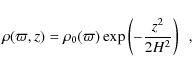
We assumed a steady-state viscous decretion disk, for which the surface density is given by (e.g., Bjorkman & Carciofi 2005)
![\begin{displaymath}\Sigma(\varpi)=\frac{\dot M}{3 \pi \alpha c_{\rm s}^2 }
\lef...
...}} \right)^{1/2}
\left[(R_0/\varpi)^{1/2}-1\right] \enspace ,
\end{displaymath}](/articles/aa/full_html/2009/36/aa10962-08/img72.png)
where
 |
(2) |
is the distance from the center of the star,
The integration constant R0 is a free parameter related to the physical size of the disk. For time-dependent models, such as those of Okazaki (2007), R0 grows with time and thus R0 is related with the age of the disk.
![]() Tau is a well-known single line binary (Harmanec 1984) and it is usually assumed that the tidal forces from the secondary
physically truncate the disk at a radius
Tau is a well-known single line binary (Harmanec 1984) and it is usually assumed that the tidal forces from the secondary
physically truncate the disk at a radius ![]() ,
corresponding to the tidal radius of the system (Whitehurst & King 1991). Assuming that the disk is sufficiently old,
,
corresponding to the tidal radius of the system (Whitehurst & King 1991). Assuming that the disk is sufficiently old,
![]() ,
in which case Eq. (1) can be written in a simple parameterized form
,
in which case Eq. (1) can be written in a simple parameterized form
where
![\begin{displaymath}\Sigma_0 = \frac{\dot M} {3 \pi \alpha c_{\rm s}^2} \left( \f...
... \right)^{1/2} \left[(R_0/R_{\rm e})^{1/2}-1\right] \enspace .
\end{displaymath}](/articles/aa/full_html/2009/36/aa10962-08/img80.png)
In Eq. (1) the disk density scale is controlled both by R0 and
the mass decretion rate is related to both the surface density and the radial velocity,
This latter quantity is difficult to obtain directly from the observations, because the outflow velocities in the inner disk are probably several orders of magnitude lower than the orbital speeds (Waters & Marlborough 1994; Hanuschik 2000,1994). However, the outflow velocity can, in principle, be determined indirectly. As discussed below, the eigenvalues of the global oscillation mode depend on the viscosity parameter ![]() .
This parameter, in turn, sets the outflow velocity (this can be seen by substituting Eq. (3) in Eq. (5)).
Therefore, if we can sufficiently constrain the global oscillation eigenvalues (see Sect. 4), the value of
.
This parameter, in turn, sets the outflow velocity (this can be seen by substituting Eq. (3) in Eq. (5)).
Therefore, if we can sufficiently constrain the global oscillation eigenvalues (see Sect. 4), the value of ![]() and, as a consequence, the decretion rate, could be obtained.
and, as a consequence, the decretion rate, could be obtained.
From the binary parameters of Table 1,
we find that the Roche radius of the system is
![]() .
Here we used the approximate formula for the Roche radius by Eggleton (1983), which is given by
.
Here we used the approximate formula for the Roche radius by Eggleton (1983), which is given by
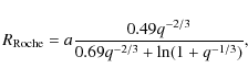
where a is the semi-major axis and q = M2/M1 is the binary mass ratio. Since the tidal radius is approximately
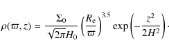
We also assumed that the disk is in vertical hydrostatic equilibrium. In this case, it can be shown that the density of isothermal disks is given by (Bjorkman & Carciofi 2005)
where
where
The radial dependence of ![]() can be determined considering that
can be determined considering that ![]() is the integral of
is the integral of ![]() in the z direction,
in the z direction,
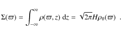
From Eqs. (3) to (9) one obtains
Before describing the global oscillation model, a few words about the HDUST solution of the gas state variables are warranted. From Eqs. (3) and (7) we see that the solutions for both the vertical hydrostatic equilibrium and the radial diffusion depends on the disk temperature. In a recent work, Carciofi & Bjorkman (2008) studied the hydrodynamics of non-isothermal viscous Keplerian disks and found that the density structure of such disks can strongly deviate from the simple isothermal solution of Eqs. (1) and (7). The dissimilarities between the two solutions are most marked for the inner disk (
The models presented in this work have an isothermal density structure but are not isothermal, because for the assumed density distribution HDUST calculates the full NLTE and radiative equilibrium problem, thereby providing the gas temperature as a function of position in the disk. Carciofi & Bjorkman (2008) demonstrated that such mixed models are a much better approach to the problem than a purely isothermal model. The reason why an isothermal density structure was assumed in this work lies in the fact that at the moment only an isothermal solution for the global disk oscillations is available. Lifting this inconsistency between the calculated temperature distribution and the assumed density will be left for future work.
To model the V/R variations and the VLTI/AMBER observations reported in Paper I, Eq. (3) must be modified according to the global oscillation model of Okazaki (1997) and Papaloizou et al. (1992).
In calculating the gravitational potential, we take into
account the quadrupole contribution due to the rotational deformation
of the rapidly rotating Be primary (Papaloizou et al. 1992). We also take into
account the azimuthally averaged tidal potential (Hirose & Osaki 1993).
The potential is then given by
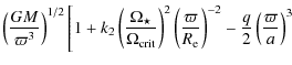
![$\displaystyle \psi \simeq -\frac{GM}{\varpi} \left\{ 1 + k_{2}\left(\frac
{\Ome...
...i}{a} \left[ 1 + \frac{1}{4}{\left(\frac{\varpi}{a}
\right)}^2\right] \right\},$](/articles/aa/full_html/2009/36/aa10962-08/img97.png)
where
The radial distribution of the rotational angular velocity
![]() is derived from the equation of motion in the radial direction, and is written explicitly as
is derived from the equation of motion in the radial direction, and is written explicitly as
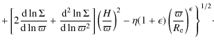
![$\displaystyle \left. + \frac{{\rm d} \ln \Sigma}{{\rm d} \ln \varpi}\left(\frac...
...\right)^{2} -\eta \left(\frac{\varpi}{R_{\rm e}}\right)^\epsilon \right]^{1/2},$](/articles/aa/full_html/2009/36/aa10962-08/img104.png)
under the approximation
where
![$\displaystyle \left[ 2 \Omega \left( 2\Omega + \varpi \frac{{\rm d}
\Omega}{{\rm d} \varpi} \right) \right]^{1/2}$](/articles/aa/full_html/2009/36/aa10962-08/img111.png)
The perturbed surface density is obtained by superposing a linear m=1 perturbation on the above unperturbed state (Eq. (3)) in the form of normal mode of frequency
![$\displaystyle \left[ i(\omega-\Omega)+v_{\varpi}{d \over {d \varpi}} \right]
{\...
...rpi\Sigma v_
{\varpi}^{\prime} \right)
-{{i v_\phi^{\prime}} \over \varpi} = 0,$](/articles/aa/full_html/2009/36/aa10962-08/img116.png)
![$\displaystyle c_{\rm s}^2 {{\rm d} \over {{\rm d} \varpi}}\left( {\Sigma^{\prim...
...er {{\rm d} \varpi}}
\right] v_{\varpi}^{\prime} - 2\Omega v_\phi^{\prime} = 0,$](/articles/aa/full_html/2009/36/aa10962-08/img117.png)
![$\displaystyle \hspace*{4em}
+\left[ i(\omega-\Omega)+{v_{\varpi} \over \varpi}+v_{\varpi}{d
\over {d \varpi}} \right] v_\phi^{\prime} = 0,$](/articles/aa/full_html/2009/36/aa10962-08/img119.png)
where
It is instructive to consider the effects of some parameters on the m=1 oscillations before solving the perturbation equations. For
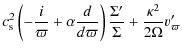
simplicity, we first neglect viscous terms. In this case, the local dispersion relation is obtained from Eqs. (15)-(17) as
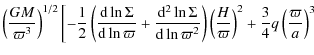
where k is the radial wave number. The propagation region, where k is a real number, is given as the region for which
![$\displaystyle \Omega - \kappa \left[1-\left(\frac{v_{\varpi}}{c_{\rm s}}
\right)^2 \right]^{1/2}$](/articles/aa/full_html/2009/36/aa10962-08/img128.png)
![$\displaystyle \left. +k_2 \left(\frac{\Omega_\star}{\Omega_{\rm crit}}\right)^
...
...)^\epsilon
+\frac{1}{2}\left(\frac{v_{\varpi}}{c_{\rm s}}\right)^2 \right]\cdot$](/articles/aa/full_html/2009/36/aa10962-08/img130.png)
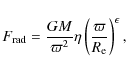
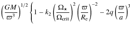
Here, the first, second, and third terms are due to the pressure gradient force, tidal force and the quadrupole contribution of the potential around the deformed star, respectively. The fourth term is due to the radiation force and the last term is the contribution due to advection. Near the star, the quadrupole term and the radiation term play the major role. Thus, the eigenfrequency is mainly determined by these terms and the pressure gradient term. The larger the contribution of the quadrupole term and the radiation term and/or the smaller the sound speed (or temperature), the higher the eigenfrequency. On the other hand, the other terms, i.e., the tidal term and the advective term, as well as the pressure gradient term affect the oscillation behavior in the outer part of the disk. The larger the contribution of these terms, the less the eigenmode is confined, and vice versa.
Next, we consider the effects of viscosity. When the
mass-decretion rate ![]() and the surface density at the inner
disk radius
and the surface density at the inner
disk radius ![]() are fixed, the radial velocity
are fixed, the radial velocity
![]() is
proportional to the viscosity parameter
is
proportional to the viscosity parameter ![]() .
Thus, one effect of
viscosity is to make the oscillation mode less confined, in terms of
the advective term. Kato et al. (1978) showed that m=1 modes in nearly
Keplerian disks, which are neutral if viscosity is neglected,
become overstable when viscous effects are taken into account. The growth rate is proportional to
.
Thus, one effect of
viscosity is to make the oscillation mode less confined, in terms of
the advective term. Kato et al. (1978) showed that m=1 modes in nearly
Keplerian disks, which are neutral if viscosity is neglected,
become overstable when viscous effects are taken into account. The growth rate is proportional to ![]() (see also Negueruela et al. 2001).
(see also Negueruela et al. 2001).
It is important to note that our model provides prograde modes for a
plausible range of parameters. The fundamental mode, in general, has
eigenfrequency of the order
![]() .
From
Eq. (19) it is obvious that
.
From
Eq. (19) it is obvious that
![]() is positive even if no
radiation force is included. Thus, there is no way to reproduce the observed V/R period of
is positive even if no
radiation force is included. Thus, there is no way to reproduce the observed V/R period of ![]() Tau by retrograde modes, which have
negative eigenfrequencies.
Tau by retrograde modes, which have
negative eigenfrequencies.
It should also be noted that linear models like ours cannot predict the amplitude of the oscillations.
Thus, for the purpose of comparison with various observations,
we will assume that the nonlinear perturbation patterns are similar to
the linear eigenfunctions obtained from the above equations,
and take the maximum value of the perturbed part of the surface density,
![]() ,
to be a free parameter,
,
to be a free parameter, ![]() .
.
3 Results
3.1 Modeling procedure
The global oscillation model described above is not a trivial problem for a radiative transfer solver. A very large number of grid cells (typically about 100 000) is needed to accurately describe the ![]() ,
z and
,
z and ![]() dependence of the density, of the gas state variables and of the radiation field (for details about the adopted cell structure in HDUST, such as radial and latitude spacing, see Carciofi & Bjorkman 2006).
Solving the radiative equilibrium and NLTE statistical equilibrium problems for each cell involves a long series of iterations to accurately determine the coupling between radiation and state variables in the dense environment of the inner disk. This, and the subsequent calculation of the observables, takes between 2 and 3 days for a single model in a cluster of 50 Pentium IV computers.
dependence of the density, of the gas state variables and of the radiation field (for details about the adopted cell structure in HDUST, such as radial and latitude spacing, see Carciofi & Bjorkman 2006).
Solving the radiative equilibrium and NLTE statistical equilibrium problems for each cell involves a long series of iterations to accurately determine the coupling between radiation and state variables in the dense environment of the inner disk. This, and the subsequent calculation of the observables, takes between 2 and 3 days for a single model in a cluster of 50 Pentium IV computers.
This is prohibitively long for the iterative procedure necessary to fit the observations.
For this reason, we initially modeled the global disk properties using a simple 2D viscous decretion model using Eqs. (3) and (7).
This 2D analysis allowed us to place initial constraints on several parameters of the system, including ![]() ,
,
![]() ,
i, and d (Sect. 3.2).
,
i, and d (Sect. 3.2).
Once a suitable 2D model was found, we used it as a starting point for the detailed 3D modeling described in Sect. 2.3. With this 3D model we performed a simultaneous analysis of the VLTI/AMBER interferometry and the V/R properties of the H I lines, that allowed us to constrain well the global disk oscillations parameters (Sect. 3.3).
3.2 Two-dimensional viscous decretion disk model
As discussed in Paper I, ![]() Tau has shown little or no secular evolution since the onset of the current V/R activity started in 1992, and it is argued that the global disk properties, basically its density scale, have been approximately constant in the period. Therefore, modeling the data with a 2D viscous decretion disk is per se a useful exercise that can provide insight into the average properties of this disk.
Tau has shown little or no secular evolution since the onset of the current V/R activity started in 1992, and it is argued that the global disk properties, basically its density scale, have been approximately constant in the period. Therefore, modeling the data with a 2D viscous decretion disk is per se a useful exercise that can provide insight into the average properties of this disk.
Initially, a set of observations that are representative of the period from 1992 through 2008 must be defined.
For both the spectral energy distribution (SED) and polarization in the 0.3-
![]() region, we used the PBO spectropolarimetric observations made in March, 1996 (Wood et al. 1997). The flux and polarization levels were scaled in order to match the average V-band flux and polarization of the period (
region, we used the PBO spectropolarimetric observations made in March, 1996 (Wood et al. 1997). The flux and polarization levels were scaled in order to match the average V-band flux and polarization of the period (
![]() ,
,
![]() %, see Paper I). To extend the SED to the IR, we used archival data from the IRAS point source catalog (Beichman et al. 1988) and the 2MASS catalog (Cutri et al. 2003).
%, see Paper I). To extend the SED to the IR, we used archival data from the IRAS point source catalog (Beichman et al. 1988) and the 2MASS catalog (Cutri et al. 2003).
Because the line profiles are variable and strongly dependent on the disk asymmetries caused by the global oscillations, we fitted only the average H![]() peak separation in this period (
peak separation in this period (
![]() ,
Paper I) and the average H
,
Paper I) and the average H![]() EW (
EW (
![]() ,
Paper I).
,
Paper I).
One of the most beautiful characteristics of the viscous decretion disk model is its relatively small number of parameters. To describe the steady-state structure of the disk we need to specify the decretion rate, ![]() ,
the viscosity parameter,
,
the viscosity parameter, ![]() ,
and the age of the disk that is enclosed in the parameter R0 (Eq. (1)). We further need to specify the stellar critical velocity,
,
and the age of the disk that is enclosed in the parameter R0 (Eq. (1)). We further need to specify the stellar critical velocity,
![]() ,
which is a measure of the stellar mass and affects the disk structure by setting its scaleheight (Eq. (8)) and rotation speeds.
In the case of the disk around
,
which is a measure of the stellar mass and affects the disk structure by setting its scaleheight (Eq. (8)) and rotation speeds.
In the case of the disk around ![]() Tau we assumed, as explained in Sect. 2.3, that the disk is truncated by a companion star. This mechanism erases the information about the disk age and makes the problem undetermined. This basically means that
Tau we assumed, as explained in Sect. 2.3, that the disk is truncated by a companion star. This mechanism erases the information about the disk age and makes the problem undetermined. This basically means that ![]() ,
,
![]() and R0 are all contained in a single parameter,
and R0 are all contained in a single parameter, ![]() ,
which determines the disk density scale.
Therefore, the disk is described by only two free parameters,
,
which determines the disk density scale.
Therefore, the disk is described by only two free parameters, ![]() and
and
![]() .
In addition to these two physical parameters we must specify two geometrical parameters, the viewing angle, i, and the distance to the star, d.
.
In addition to these two physical parameters we must specify two geometrical parameters, the viewing angle, i, and the distance to the star, d.
For this analysis several tens of models were run, covering a large range of values for ![]() ,
,
![]() and i.
For each model, the value of d was computed in order to match the observed flux levels. Since d is known to be in the range between 113-
and i.
For each model, the value of d was computed in order to match the observed flux levels. Since d is known to be in the range between 113-
![]() ,
which corresponds to the accuracy in the distance determination by the Hipparcos satellite (Perryman et al. 1997), models that did not produce d in this range were discarded.
,
which corresponds to the accuracy in the distance determination by the Hipparcos satellite (Perryman et al. 1997), models that did not produce d in this range were discarded.
![\begin{figure}
\par\includegraphics[width=9cm]{10962f2.eps}
\end{figure}](/articles/aa/full_html/2009/36/aa10962-08/img140.png) |
Figure 2:
Emergent spectrum of |
| Open with DEXTER | |
Figure 2 shows the best fit to the data using the 2D viscous decretion model. This best fit was achieved for the following parameters
| |
= | ||
| i | = | ||
| = | |||
| d | = |
in addition to the fixed stellar parameters listed in the first part of Table 1. Recall that for all models the disk was truncated at
The above value for ![]() corresponds to
corresponds to
![]() .
The number density of particles can be estimated assuming a mean molecular weight of 0.6, typical for ionized gas with solar chemical composition (recall that the model have only H). We obtain a value of
.
The number density of particles can be estimated assuming a mean molecular weight of 0.6, typical for ionized gas with solar chemical composition (recall that the model have only H). We obtain a value of
![]() ,
which is characteristic of Be stars with dense disks, such as
,
which is characteristic of Be stars with dense disks, such as ![]() Sco (Carciofi et al. 2006).
Sco (Carciofi et al. 2006).
Before discussing our results, it is useful to recall the physical processes that control the emergent spectrum. In the visible, the SED depends on the spectral shape of the stellar radiation, which, for a rotating star, is controlled by the latitude-dependent effective temperature. The stellar radiation is modified by several processes in the CS disk: electron scattering, bound-free absorption and free-bound emission by H I atoms, free-free absorption and emission by free electrons, and line absorption and emission by H and other elements. The absorption and emission processes depend on the atomic occupation numbers and electron temperature, which, in turn, depend on the radiation field in a non-linear and complex way.
In the IR the SED is controlled mainly by the free-free emission of the free electrons. The continuum polarization is produced by electron scattering, but is also modified by the absorption and emission processes in the disk.
The absorption, emission and scattering of the radiation depends also on the geometry and velocity structure of the CS material. For instance, the linear polarization is strongly dependent on the number density of electrons, the disk flaring and scaleheight. The slope of the IR SED, on the other hand, depends mainly on the radial profile of the density, but also on the disk flaring and temperature distribution (Carciofi & Bjorkman 2006).
In view of the complex dependence of the emergent radiation on the stellar and disk parameters, the overall good match between the model and observations is remarkable. The model reproduces the SED longward of the Balmer jump (
![]() )
all the way down to the longest IRAS wavelength. The only part of the SED which is not well reproduced is the size of the Balmer jump. The size of the jump is too large in the model, meaning that either the amount of neutral hydrogen in the line of sight is a little overestimated or the geometry of inner disk is not well described by the model (see Sect. 4).
)
all the way down to the longest IRAS wavelength. The only part of the SED which is not well reproduced is the size of the Balmer jump. The size of the jump is too large in the model, meaning that either the amount of neutral hydrogen in the line of sight is a little overestimated or the geometry of inner disk is not well described by the model (see Sect. 4).
The predicted polarization matches the observations well. The size of the Balmer jump and the level and slope of the polarization in the Paschen continuum show good agreement. However, in the Brackett continuum the model overestimates the polarization by approximately 10%.
The best-fit model has an inclination angle of
![]() .
The fact that
.
The fact that ![]() Tau is a well-known shell star (Rivinius et al. 2006; Porter 1996) supports this finding. Figure 3 compares the model polarization for 3 different inclination angles, 83
Tau is a well-known shell star (Rivinius et al. 2006; Porter 1996) supports this finding. Figure 3 compares the model polarization for 3 different inclination angles, 83![]() ,
85
,
85![]() and 87
and 87![]() .
Differences in i as small as 2
.
Differences in i as small as 2![]() produce significant changes in the polarization, which indicates that the inclination angle is well constrained by our analysis.
produce significant changes in the polarization, which indicates that the inclination angle is well constrained by our analysis.
![\begin{figure}
\par\includegraphics[width=9cm]{10962f3.eps}
\end{figure}](/articles/aa/full_html/2009/36/aa10962-08/img151.png) |
Figure 3:
Continuum polarization for |
| Open with DEXTER | |
The extent that the CS disk modifies the stellar radiation can be assessed by comparing the model SED with the unattenuated stellar radiation in Fig. 2. Since the star is viewed close to edge on, this causes extinction of UV and visible radiation that is reemitted at longer wavelengths. Most of the reprocessed radiation escapes in the polar direction, due to the fact that the vertical optical depth is much smaller than the radial optical depth. However, a portion of this radiation will escape radially and will contribute to the large IR excess observed (![]() 3 mag at
3 mag at
![]() ).
).
The H![]() peak separation and EW for the best-fit model are 240 km s-1 and
peak separation and EW for the best-fit model are 240 km s-1 and
![]() ,
respectively, in good agreement with the average values for this time period.
We chose
,
respectively, in good agreement with the average values for this time period.
We chose
![]() as a free parameter and, therefore, no a priori assumption about the stellar mass have been made.
as a free parameter and, therefore, no a priori assumption about the stellar mass have been made.
![]() is well constrained by the model, as both the CS emission lines and the continuum polarization depend on this value (recall that
is well constrained by the model, as both the CS emission lines and the continuum polarization depend on this value (recall that
![]() affects the disk scaleheight).
affects the disk scaleheight).
![]() and the assumed
and the assumed
![]() give a stellar mass of
give a stellar mass of
![]() ,
in agreement with Harmanec (1984). This further supports the values of the parameters adopted for the central star.
,
in agreement with Harmanec (1984). This further supports the values of the parameters adopted for the central star.
The good fit that was obtained using a relatively simple model provides strong observational support to our assumptions.
The power-law description for the surface density proved successful in determining the slope of the IR SED, and the hydrostatic equilibrium assumption successfully determined the correct shape and level of the continuum polarization. Therefore, we conclude that a steady-state viscous decretion disk, truncated at
![]() ,
is a good description for the average properties of the CS disk around
,
is a good description for the average properties of the CS disk around ![]() Tau.
Tau.
3.3 Global oscillation model
![\begin{figure}
\par\includegraphics[width=9cm]{10962f4.eps}
\end{figure}](/articles/aa/full_html/2009/36/aa10962-08/img157.png) |
Figure 4:
|
| Open with DEXTER | |
We now present the analysis of the VLTI/AMBER observations and the V/R properties of ![]() Tau using the global oscillation model.
In addition to the parameters
Tau using the global oscillation model.
In addition to the parameters ![]() ,
,
![]() ,
d, and i, discussed above, we now take into consideration the parameters k2,
,
d, and i, discussed above, we now take into consideration the parameters k2, ![]() ,
,
![]() ,
,
![]() and the weak line force, so that the m=1 density perturbation within the disk can be modeled.
Also, the time-dependent position of the m=1 perturbation pattern with respect to the direction of the observer, described by the parameter
and the weak line force, so that the m=1 density perturbation within the disk can be modeled.
Also, the time-dependent position of the m=1 perturbation pattern with respect to the direction of the observer, described by the parameter ![]() ,
must be determined (see Fig. 1).
,
must be determined (see Fig. 1).
Different aspects of the solution are illustrated in Figs. 4 to 9, and the
parameters of the best fit obtained are summarized in Table 1.
Before continuing to describe the results, some explanations about the modeling procedure are warranted.
For a given model, HDUST computes the emergent spectrum for an observer whose position is specified by i and ![]() .
To simulate the temporal dependence of the observables as the density wave precesses around the star, we computed, for a given i, the emergent spectrum for several values of
.
To simulate the temporal dependence of the observables as the density wave precesses around the star, we computed, for a given i, the emergent spectrum for several values of ![]() .
The global oscillation parameters used in the simulation are then evaluated by comparing the theoretical amplitude and shape of the V/R cycle to the observations.
.
The global oscillation parameters used in the simulation are then evaluated by comparing the theoretical amplitude and shape of the V/R cycle to the observations.
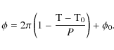
The time-dependent position of the density wave is related to the V/R phase as follows. According to the convention of Paper I, the V/R phase, ![]() ,
is defined such that
,
is defined such that ![]() at the V/R maximum. The ephemerides of the V/R cycle, given by the period, P, and the modified Julian date for
at the V/R maximum. The ephemerides of the V/R cycle, given by the period, P, and the modified Julian date for ![]() ,
T0, were determined in Paper I and are listed in Table 1.
We introduce the parameter
,
T0, were determined in Paper I and are listed in Table 1.
We introduce the parameter ![]() ,
which gives the position of an arbitrary point of the spiral pattern at
,
which gives the position of an arbitrary point of the spiral pattern at ![]() .
We chose this point to be the minimum of the density perturbation pattern at the base of the disk. The angle
.
We chose this point to be the minimum of the density perturbation pattern at the base of the disk. The angle ![]() is related to the phase by
is related to the phase by
 |
(20) |
(Note that the angle
This equation gives the position of the minimum of the density pattern at the base of the star as a function of time. For a given model, a value of
3.3.1 Constraints from the V/R Observations
Figure 4 shows the best fit to the V/R cycle of the H![]() ,
Br
,
Br![]() and Br15 lines.
For H
and Br15 lines.
For H![]() ,
the model reproduces the first part of the V/R cycle (
,
the model reproduces the first part of the V/R cycle (
![]() ), including the shape of the curve and the observed V/R maxima and minima. In the second half of the cycle, between
), including the shape of the curve and the observed V/R maxima and minima. In the second half of the cycle, between
![]() ,
the observed V/R ratio departs from the quasi-sinusoidal shape that is characteristic of the first half (Paper I), and this is not reproduced by the model.
,
the observed V/R ratio departs from the quasi-sinusoidal shape that is characteristic of the first half (Paper I), and this is not reproduced by the model.
The behavior of the V/R properties of the IR lines are similar to that of H![]() ,
but the smaller number of observations make the results less conclusive. Unfortunately, there are only three observations in the first half of the cycle, but their V/R ratios agree with the predicted values (see points for
,
but the smaller number of observations make the results less conclusive. Unfortunately, there are only three observations in the first half of the cycle, but their V/R ratios agree with the predicted values (see points for
![]() ).
The second half of the cycle is better covered.
For Br
).
The second half of the cycle is better covered.
For Br![]() ,
the model seems to reproduce the data, but the V/R values tend to cluster above the predicted curve, with the exception of the two points for
,
the model seems to reproduce the data, but the V/R values tend to cluster above the predicted curve, with the exception of the two points for
![]() .
For Br15, all the data points are above the predicted values in the second half of the cycle.
.
For Br15, all the data points are above the predicted values in the second half of the cycle.
One interesting feature of the observations that is clearly seen in Fig. 4, are the phase differences between the cycles of different lines. These phase differences have been already observed in ![]() Tau by Wisniewski et al. (2007), who suggested that they might be associated with the helicity of the global oscillation.
The idea behind this suggestion is that the more optically thin infrared lines form closer to the star in the disk, whereas the H
Tau by Wisniewski et al. (2007), who suggested that they might be associated with the helicity of the global oscillation.
The idea behind this suggestion is that the more optically thin infrared lines form closer to the star in the disk, whereas the H![]() line forming region extends further out into the disk. Because of the strong helicity of the density perturbation pattern (see, e.g., Fig. 5), the average azimuthal morphology of the inner disk is quite different than the morphology of the outer disk. Therefore, the observed phase differences would be a result of the different average morphology of each line formation site.
line forming region extends further out into the disk. Because of the strong helicity of the density perturbation pattern (see, e.g., Fig. 5), the average azimuthal morphology of the inner disk is quite different than the morphology of the outer disk. Therefore, the observed phase differences would be a result of the different average morphology of each line formation site.
![\begin{figure}
\par\mbox{\includegraphics[height=3.8cm]{10962f5a.eps}\includegra...
...ace*{5mm}\includegraphics[width=8.0cm]{10962f5d.eps}\hspace*{5mm}}\end{figure}](/articles/aa/full_html/2009/36/aa10962-08/img167.png) |
Figure 5:
Comparison of the results for modes with different degrees of confinement. The top left plot shows the density perturbation pattern for the V/R parameters of Table 1. The figure depicts the disk as seen from above, in which case the density wave precesses counter-clockwise. A more confined mode, with a weak line force of
|
| Open with DEXTER | |
The phase differences between the H![]() and Br
and Br![]() lines are well reproduced by our models, which provides convincing evidence in support to a spiral morphology of the density perturbation pattern in the disk of
lines are well reproduced by our models, which provides convincing evidence in support to a spiral morphology of the density perturbation pattern in the disk of ![]() Tau. The phase of the Br15 line is not well reproduced, however. This line is formed in the very inner part of the disk and it seems, therefore, that the global oscillation model does not describe correctly the shape of the spiral pattern in this region.
In Fig. 4, the dashed red line shows the model V/R curve of the Br15 line shifted in phase by -0.2. This artificially displaced curve reproduces the observations.
This may indicate that the model predicts the correct amplitude of the oscillations in the inner disk, even though the shape, which sets the phase, is not correct.
Tau. The phase of the Br15 line is not well reproduced, however. This line is formed in the very inner part of the disk and it seems, therefore, that the global oscillation model does not describe correctly the shape of the spiral pattern in this region.
In Fig. 4, the dashed red line shows the model V/R curve of the Br15 line shifted in phase by -0.2. This artificially displaced curve reproduces the observations.
This may indicate that the model predicts the correct amplitude of the oscillations in the inner disk, even though the shape, which sets the phase, is not correct.
![\begin{figure}
\par\includegraphics[width=13cm,clip,angle=270]{10962f6.eps}
\end{figure}](/articles/aa/full_html/2009/36/aa10962-08/img168.png) |
Figure 6:
Fitting of the interferometric observations for the spectral region around the Br |
| Open with DEXTER | |
As mentioned above, the global oscillation model failed to reproduce the H![]() V/R cycle for
V/R cycle for
![]() .
However, this may not be a problem with the global oscillation model, since the
.
However, this may not be a problem with the global oscillation model, since the
![]() phase interval is where the complex triple-peaked H
phase interval is where the complex triple-peaked H![]() profiles become more prominent. Paper I presented evidence that the triple-peak anomaly arises from the outermost part of the disk, and that it is probably a line-of-sight effect owing to the large inclination angle of the system.
The failure to reproduce this part of the V/R cycle is likely due to the fact that a physical process is missing in our analysis.
profiles become more prominent. Paper I presented evidence that the triple-peak anomaly arises from the outermost part of the disk, and that it is probably a line-of-sight effect owing to the large inclination angle of the system.
The failure to reproduce this part of the V/R cycle is likely due to the fact that a physical process is missing in our analysis.
Figure 5 illustrates the properties of our solution for the disk global oscillation. The oscillation mode is subject to two very stringent constraints: it must have a precessing period equal to the observed V/R period (1429 days, see Paper I) and it must be able to reproduce the observed amplitude of the V/R variations. This latter requirement is associated with the degree of confinement of the mode, which essentially means how far out into the disk the perturbation goes. Figure 5 compares the theoretical V/R curve for two modes with the same precession period but different degrees of confinement. The model shown in the top left is the best fit model of Table 1. This model corresponds to a mode with a small degree of confinement, in which the oscillations extend all the way down to the outer rim of the disk. The other model is shown as an example of a mode that also has the same precession period but it is much more confined. From the comparison of the predicted V/R ratios for each mode (bottom panel of Fig. 5) we see that this latter mode can be readily discarded on the basis that it cannot account for the observed amplitude of the V/R variations.
3.3.2 Contraints from the AMBER/VLTI observations
Perhaps the strongest evidence in support of the global oscillation scenario comes from the very good fit of the interferometric data.
The formal fit of the observed visibilities and phases is shown in Fig. 6 for three baselines (marked as A, B and C, see Fig. 7 for their orientation with respect to the disk). In the figure, the left column shows the phases and the middle column the square visibilities for each baseline. Because of the poor absolute calibration of our dataset, both observables were normalized to the value obtained in the continuum. The difference in amplitude of the different profiles are explained by both the baseline lengths (93 m, 53 m and 130 m, respectively) and orientation (
![]() ,
,
![]() and
and
![]() East from North, respectively). For instance, baseline A corresponds to an orientation close to the minimum elongation axis of the disk, which explains the small drop in visibility. The quality of the fit is quantitatively expressed by the
East from North, respectively). For instance, baseline A corresponds to an orientation close to the minimum elongation axis of the disk, which explains the small drop in visibility. The quality of the fit is quantitatively expressed by the ![]() map shown in the right column.
map shown in the right column.
![\begin{figure}
\par\mbox{\includegraphics[height=4.5cm]{10962f7a.eps} \includegr...
...g.eps} \includegraphics[width=4.5cm]{10962f7h.eps}\hspace*{4.5cm}}\end{figure}](/articles/aa/full_html/2009/36/aa10962-08/img176.png) |
Figure 7:
Top left: density perturbation pattern of our best-fit model, as seen from above the disk. The line of sight towards the observer is marked for 5 V/R phases. The VLTI/AMBER observations corresponds to |
| Open with DEXTER | |
For illustration purposes, we converted the three interferometric phases into an astrometric displacement for each spectral bin across the line (top-right panel of Fig. 6). Open and filled symbols indicate the displacement along the disk at minimum and maximum elongation axes, respectively. The typical S-shape astrometric signature of a rotating disk is clearly distorted: the redshifted part of the disk extends further away from the central star than the blueshifted part (300 ![]() as and
as and ![]() as respectively). This is a direct, illustrative proof of the presence of an asymmetry in the disk.
as respectively). This is a direct, illustrative proof of the presence of an asymmetry in the disk.
The fits of the visibilities and phases were carried out in the following way. For a given disk model and inclination angle, we computed synthetic images for several wavelengths around the Br![]() line (see Fig. 7) for several values of
line (see Fig. 7) for several values of ![]() ,
corresponding to different V/R phases. This set of synthetic images were then rotated for several values of
,
corresponding to different V/R phases. This set of synthetic images were then rotated for several values of ![]() ,
corresponding to different orientations of the disk in the skyplane. Next, the visibilities and phases for each of the modified images were computed and compared to the observed visibilities and phases. A
,
corresponding to different orientations of the disk in the skyplane. Next, the visibilities and phases for each of the modified images were computed and compared to the observed visibilities and phases. A ![]() minimization procedure was carried out that produced the values of
minimization procedure was carried out that produced the values of ![]() and
and ![]() that best fitted the data
that best fitted the data![]() . Finally, we manually explored the parameter d in the range 113-148 pc. However, we have always found that this had only a marginal impact on our fit and, therefore, we chose to use the distance determined from the 2D analysis, d=126 pc.
. Finally, we manually explored the parameter d in the range 113-148 pc. However, we have always found that this had only a marginal impact on our fit and, therefore, we chose to use the distance determined from the 2D analysis, d=126 pc.
This procedure was repeated for several disk models and inclination angles. An analysis of the flux, polarization and V/R properties was also carried out for the same models. The model parameters of Table 1 correspond to the values that best reproduced all data analyzed, including the interferometry.
This analysis indicates that the interferometry is much more sensivite to some model parameters than others. The most sensitive parameter, and hence the best constrained, is undoubtedly the disk orientation
![]() .
As discussed in Paper I, this value agrees well with previous polarimetric and interferometric determinations.
In particular, it is compatible with the recently published value
.
As discussed in Paper I, this value agrees well with previous polarimetric and interferometric determinations.
In particular, it is compatible with the recently published value
![]() ,
obtained in the
,
obtained in the
![]() band with the CHARA array (Gies et al. 2007). Additionally, as shown in the middle-right panel of Fig. 6, the overall size of our models also agrees with that measured by Gies et al. (2007). Note that the CHARA and VLTI/AMBER estimates are independent because Gies et al. (2007) used absolutely calibrated broad band visibilities, whereas we used differential phases and visibilities across a line.
band with the CHARA array (Gies et al. 2007). Additionally, as shown in the middle-right panel of Fig. 6, the overall size of our models also agrees with that measured by Gies et al. (2007). Note that the CHARA and VLTI/AMBER estimates are independent because Gies et al. (2007) used absolutely calibrated broad band visibilities, whereas we used differential phases and visibilities across a line.
The ![]() map of Fig. 6 shows that the parameter
map of Fig. 6 shows that the parameter ![]() is not as well constrained. From the fit we found that the position of the density wave at the time of the observation is
is not as well constrained. From the fit we found that the position of the density wave at the time of the observation is
![]() .
The large uncertainty comes from the combined effects of the high inclination of the disk and the fact that the density perturbations are spread over a large range in azimuth (see Fig. 7).
Using Eq. (21) we found that the position of the density wave at
.
The large uncertainty comes from the combined effects of the high inclination of the disk and the fact that the density perturbations are spread over a large range in azimuth (see Fig. 7).
Using Eq. (21) we found that the position of the density wave at ![]() ,
as given by the interferometry, is
,
as given by the interferometry, is
![]() .
Despite this large uncertainly, this value is in agreement with our best-fit value of
.
Despite this large uncertainly, this value is in agreement with our best-fit value of
![]() obtained primarily from the fit of the V/R phases.
We emphasize that spectroscopic and interferometric determinations of the
obtained primarily from the fit of the V/R phases.
We emphasize that spectroscopic and interferometric determinations of the ![]() are completely independent, making the above agreement relevant.
are completely independent, making the above agreement relevant.
The analysis of the interferometric data for different values of i (not shown) largely confirms the value for the inclination angle obtained from the 2D model (Sect. 3.2). In addition, interferometry has allowed us to lift a historical degeneracy in the determination of i. Recall from Fig. 1 that the inclination angle goes from 0 to
![]() .
For
.
For
![]() the top of the disk is facing the observer and the contrary is true for
the top of the disk is facing the observer and the contrary is true for
![]() .
In the case of an axisymmetric disk, it is really difficult to distinguish between
.
In the case of an axisymmetric disk, it is really difficult to distinguish between
![]() and
and
![]() .
For an infinitely thin disk this distinction is impossible, since the disk aspect would be identical for the two cases. For a disk of non-zero geometrical thickness, radiative transfer effects create subtle differences in the aspect of each disk, but the differences are probably too small to be detected. However, for a non-axisymmetric disk this distinction is possible, provided two conditions are fulfilled:
1) spatially and spectrally resolved observations are available in order to determine the rotation direction of the disk in the plane of the sky, so that the northward direction can be defined; and
2) the disk asymmetry is chiral, i.e., the disk is not superimposable on its mirror image (we adopt the usual convention that the angular momentum vector points north).
.
For an infinitely thin disk this distinction is impossible, since the disk aspect would be identical for the two cases. For a disk of non-zero geometrical thickness, radiative transfer effects create subtle differences in the aspect of each disk, but the differences are probably too small to be detected. However, for a non-axisymmetric disk this distinction is possible, provided two conditions are fulfilled:
1) spatially and spectrally resolved observations are available in order to determine the rotation direction of the disk in the plane of the sky, so that the northward direction can be defined; and
2) the disk asymmetry is chiral, i.e., the disk is not superimposable on its mirror image (we adopt the usual convention that the angular momentum vector points north).
Both of the above conditions are fulfilled for ![]() Tau.
The VLTI/AMBER observations unambiguously determine that the western side of the disk approaches the Earth. Thus, according to the definition of north and the value of
Tau.
The VLTI/AMBER observations unambiguously determine that the western side of the disk approaches the Earth. Thus, according to the definition of north and the value of ![]() derived from the interferometry, we know that the north of the system is oriented
derived from the interferometry, we know that the north of the system is oriented
![]() east of celestial north. Condition 2 is also fulfilled, since the disk is highly non-axisymmetric because of the spiral density perturbation produced by the global m=1 oscillation. From the detailed model fitting of the interferometric observations, we found that the model with viewing angle
east of celestial north. Condition 2 is also fulfilled, since the disk is highly non-axisymmetric because of the spiral density perturbation produced by the global m=1 oscillation. From the detailed model fitting of the interferometric observations, we found that the model with viewing angle
![]() (
(
![]() )
fits the observations better than the corresponding model with
)
fits the observations better than the corresponding model with
![]() (
(
![]() ,
see also differences between the models in Fig. 6). Therefore, the VLTI/AMBER data allow us to determine that the bottom part of the disk of
,
see also differences between the models in Fig. 6). Therefore, the VLTI/AMBER data allow us to determine that the bottom part of the disk of ![]() Tau faces the Earth. Note that this degeneracy is nearly impossible to be lifted with broadband interferometry data only, such as the CHARA data shown in the right-middle panel of Fig. 6. We believe that this is the first time the degeneracy in the determination of i was lifted for a Be star.
Tau faces the Earth. Note that this degeneracy is nearly impossible to be lifted with broadband interferometry data only, such as the CHARA data shown in the right-middle panel of Fig. 6. We believe that this is the first time the degeneracy in the determination of i was lifted for a Be star.
3.3.3 Geometrical considerations
The geometrical properties of ![]() Tau derived above are illustrated in Fig. 7. The top left panel shows the density perturbation pattern, as seen from above the disk. The figure marks the position of the observer's line of sight for 5 V/R phases. The
Tau derived above are illustrated in Fig. 7. The top left panel shows the density perturbation pattern, as seen from above the disk. The figure marks the position of the observer's line of sight for 5 V/R phases. The ![]() line of sight corresponds to the time of the interferometric observations.
The top center panel is a sketch of the disk density projected onto the skyplane at the time of the VLTI/AMBER observations.
The synthetic image for the IR continuum (top right panel) mimics the projected disk density as expected. The bottom panels of Fig. 7 show model images for different wavelengths across the Br
line of sight corresponds to the time of the interferometric observations.
The top center panel is a sketch of the disk density projected onto the skyplane at the time of the VLTI/AMBER observations.
The synthetic image for the IR continuum (top right panel) mimics the projected disk density as expected. The bottom panels of Fig. 7 show model images for different wavelengths across the Br![]() line. The combination of the disk asymmetries and the effects of rotation generates a very complex brightness distribution.
line. The combination of the disk asymmetries and the effects of rotation generates a very complex brightness distribution.
From Fig. 7 we see that in December 2006 (![]() )
the base of the spiral arm was behind the star, but the bulk of the material was located in the north-east.
This is consistent with the V/R < 1 value at the period of VLTI/AMBER observations (recall that the western side of the disk is approaching us).
)
the base of the spiral arm was behind the star, but the bulk of the material was located in the north-east.
This is consistent with the V/R < 1 value at the period of VLTI/AMBER observations (recall that the western side of the disk is approaching us).
3.3.4 Polarization and flux
![\begin{figure}
\par\includegraphics[width=8.5cm,clip]{10962f8.eps}
\end{figure}](/articles/aa/full_html/2009/36/aa10962-08/img189.png) |
Figure 8:
Emergent spectrum from |
| Open with DEXTER | |
![\begin{figure}
\par\includegraphics[width=8.5cm,clip]{10962f9.eps}
\end{figure}](/articles/aa/full_html/2009/36/aa10962-08/img190.png) |
Figure 9: Temporal evolution of the polarization across the V/R phase. The model polarization (line) is compared with the observations (points with error bars). |
| Open with DEXTER | |
Besides the line V/R variations, the model also predicts flux and polarization variations across one V/R cycle.
This can be readily seen from Fig. 8, where we compare the observed SED, polarization spectrum and H![]() line profile with the model predictions for different phases. The polarization variations are further illustrated in Fig. 9.
line profile with the model predictions for different phases. The polarization variations are further illustrated in Fig. 9.
What causes the variations in polarization is the occultation of part of the disk by the star in this nearly edge on system. The models show that the polarization comes mainly from the region of the disk between
![]() to
to
![]() .
From the diagram in Fig. 7, we see that the bulk of the density between those radii is in front of the star for
.
From the diagram in Fig. 7, we see that the bulk of the density between those radii is in front of the star for
![]() .
Since polarization is roughly proportional to the number of scatterers, the polarization is expected to be greatest at this phase, as in indeed the case (Fig. 9). As the density perturbation pattern precesses, eventually the bulk of the material will move behind the star at
.
Since polarization is roughly proportional to the number of scatterers, the polarization is expected to be greatest at this phase, as in indeed the case (Fig. 9). As the density perturbation pattern precesses, eventually the bulk of the material will move behind the star at
![]() .
The light scattered by this material will be partially absorbed by the star causing a decrease in the polarization.
.
The light scattered by this material will be partially absorbed by the star causing a decrease in the polarization.
In Fig. 9 the predicted modulation of the polarization is compared to the observations (data from Paper I). We folded the data into phase using the V/R ephemerides of Table 1. We plot only observations from 1992 to 2004. The polarization data seems to present a big challenge to the model. The model predicts large polarization variations of up to 40%, and this is not observed. We will come back to this important point in Sect. 4.
The flux excess in visible wavelengths comes from light emitted by the recombination of a free electron with a proton, commonly called bound-free radiation. The recombination rates are roughly proportional to the square of the density and fall very rapidly with distance from the star. Thus the bulk of excess flux in the visible comes from a very small region of the disk, out to approximately 2 stellar radii.
If we consider this small region, the density enhancement due to the global oscillations is behind the star for
![]() and in front of it for
and in front of it for
![]() ,
just the opposite situation described above for the polarization (Fig. 7). This explains why the flux is smaller for
,
just the opposite situation described above for the polarization (Fig. 7). This explains why the flux is smaller for ![]() in Fig. 8 whereas the polarization is larger. The model does not predict important variations in the IR fluxes (second panel of Fig. 8) because in this case the emission comes from a much larger fraction of the disk and occultation by the star has a smaller effect.
in Fig. 8 whereas the polarization is larger. The model does not predict important variations in the IR fluxes (second panel of Fig. 8) because in this case the emission comes from a much larger fraction of the disk and occultation by the star has a smaller effect.
Unfortunately, to our knowledge no systematic photometric monitoring was carried out for ![]() Tau after the onset of the V/R variations in 1992, so our predictions for the brightness variations cannot be tested at the moment.
Tau after the onset of the V/R variations in 1992, so our predictions for the brightness variations cannot be tested at the moment.
We end this section with a discussion about the role of the parameter ![]() in the 3D analysis. When the global oscillations are considered,
in the 3D analysis. When the global oscillations are considered, ![]() represents the azimuthally averaged density scale of the disk. We found from our 3D analysis a value of
represents the azimuthally averaged density scale of the disk. We found from our 3D analysis a value of ![]() 25% larger than that obtained from the 2D analysis (see Sect. 3.2).
25% larger than that obtained from the 2D analysis (see Sect. 3.2).
4 Discussion
The analysis of the data using the global oscillation scenario proposed by Okazaki (1997) and Papaloizou et al. (1992) shows that this model has both strong and weak points.
We were able to reproduce many observational characteristics of ![]() Tau. Of particular relevance is the overall good fit of the V/R cycles of H
Tau. Of particular relevance is the overall good fit of the V/R cycles of H![]() and Br
and Br![]() lines and the excellent fit to the VLTI/AMBER observations.
This favorable outcome of the analysis implies that the general morphology of the asymmetries in the disk of
lines and the excellent fit to the VLTI/AMBER observations.
This favorable outcome of the analysis implies that the general morphology of the asymmetries in the disk of ![]() Tau are correctly reproduced by the model, at least in the regions of the disk where most
of the H
Tau are correctly reproduced by the model, at least in the regions of the disk where most
of the H![]() and Br
and Br![]() radiation originates.
In addition, the fit of the observed phase difference between the V/R cycles of H
radiation originates.
In addition, the fit of the observed phase difference between the V/R cycles of H![]() and Br
and Br![]() strongly supports the theoretical prediction that the density wave has a helical shape.
strongly supports the theoretical prediction that the density wave has a helical shape.
However, two weak points of the model stand out from the analysis. The model did not reproduce the phase of the V/R cycle of the Br15 line, even though the amplitude was reproduced. Also, the model predicts large variations in polarization across one V/R cycle that are not observed. Both the Br15 line and the polarization share a common property: both are formed in the very inner part of the envelope within a few stellar radii.
Considering the above discussion, a pattern emerges. Observables that trace the larger scale of the disk (H![]() and Br
and Br![]() )
are reproduced by the model, whereas observables that map the inner disk (Br15 and polarization) are not.
This suggests that the global oscillation model fails to reproduce the shape and/or amplitude of the density wave in the inner disk, but it does reproduce the general features of the outer disk.
)
are reproduced by the model, whereas observables that map the inner disk (Br15 and polarization) are not.
This suggests that the global oscillation model fails to reproduce the shape and/or amplitude of the density wave in the inner disk, but it does reproduce the general features of the outer disk.
We must bear in mind that there are at least two alternative explanations as to why the model does not fit the Br15 V/R cycle. First, the site for line formation, as calculated by HDUST may be wrong. If the size of the Br15 line emitting region were larger in the models, then the phase difference would have been smaller. Second, there are other physical processes that affect the structure of the inner disk, and these may also contribute to this discrepancy. For example, the non-isothermal effects on the disk surface density calculated by Carciofi & Bjorkman (2008). Also, the fact that the disk is unlikely to be fed by a smooth mass transfer from the star, but instead by a series of outbursts (e.g. Rivinius et al. 1998). In this case the steady-state viscous decretion disk would not be a good representation for the inner disk.
The simultaneous constraints of both the period and mode confinement, together with
a sophisticated modeling, allowed us to place more stringent limits on the V/R parameters than the previous analyzes (e.g., Vakili et al. 1998).
However, there are still uncertainties in some parameters. This is particularly true for the adopted hypothetical radiative force used to adjust the oscillation period.
There is also uncertainty arising from the fact that we cannot constrain
each parameter independently. For example, a larger value of rotation parameter
![]() makes the mode more confined, whereas the mode becomes less confined for a larger value of viscosity parameter
makes the mode more confined, whereas the mode becomes less confined for a larger value of viscosity parameter ![]() .
Thus, a similar good fit can be obtained for different sets of
.
Thus, a similar good fit can be obtained for different sets of
![]() and
and ![]() .
In order to remove such a degeneracy, a more precise determination of the basic stellar parameters must be made.
.
In order to remove such a degeneracy, a more precise determination of the basic stellar parameters must be made.
5 Conclusions
We successfully completed a very detailed modeling of the Be star ![]() Tau, using a large set of observations that were reported in the first paper of this series.
Tau, using a large set of observations that were reported in the first paper of this series.
![]() Tau provides a unique opportunity for testing theoretical ideas about disk formation and structure and about the origin of V/R variations.
First, the disk is known to have its global properties constant since at least 1992.
Second, the presence of the binary companion makes it reasonable to assume that the disk is truncated at the tidal radius of the system. Finally, the inclination angle of the disk is very well constrained.
Tau provides a unique opportunity for testing theoretical ideas about disk formation and structure and about the origin of V/R variations.
First, the disk is known to have its global properties constant since at least 1992.
Second, the presence of the binary companion makes it reasonable to assume that the disk is truncated at the tidal radius of the system. Finally, the inclination angle of the disk is very well constrained.
We assumed that the unperturbed disk structure is that of a steady-state (i.e., constant decretion rate) viscous Keplerian disk. We further assume that the disk is in vertical hydrostatic equilibrium, and to describe the density perturbations we adopted the global oscillation model of Okazaki (1991) and Papaloizou et al. (1992).
We employed the computer code HDUST of Carciofi & Bjorkman (2006) to solve the coupled problems of radiative transfer, radiative equilibrium and statistical equilibrium and we fitted, in a simultaneous and self-consistent way, all of the available observations, including the recent VLTI/AMBER observations made in December 2006.
The main conclusions of this work are:
- We obtained an excellent fit of the global, time averaged properties of the disk. From the theoretical point of view, this represents strong evidence that the viscous decretion disk scenario is the mechanism responsible for the formation of the CS disk of Tau.
- The agreement between the model predictions and the VLTI/AMBER observations and the acceptable fit of the V/R cycle of the H
 and Br
 lines represent the first fairly comprehensive quantitative test of the global oscillation scenario. By fitting the spatially resolved interferometric observations we showed that the model can reproduce the general features of the outer disk quite well. In particular, this demonstrates that the density wave is a spiral, as predicted.
- The model failed to reproduce the V/R cycle of the Br15 line and predicted a large variation in the polarization during a V/R cycle, which is not observed. Since both the Br15 line and the polarization comes from the inner disk within a few stellar radii, this suggests that the global oscillation model does not predict the correct geometry in this region. However, other possibilities for the discrepancy between the model and the observations exist, including non-isothermal effects in the inner disk structure and perturbations of the inner disk by outbursts. A detailed analysis necessary to test both ideas will be left to future work.
- With the aid of the VLTI/AMBER observations we have, for the first time, completely determined the geometrical properties of a Be star system. Non-spatially resolved determinations of the inclination angle (as, for instance, obtained from polarization studies) cannot distinguish between
 (i.e., a disk whose northern face is towards the Earth) and
 (i.e., a disk whose southern face is towards the Earth).
The detailed fit of the interferometric data allowed us to determine that the inclination angle of
Tau is
(i.e., a disk whose southern face is towards the Earth).
The detailed fit of the interferometric data allowed us to determine that the inclination angle of
Tau is
 ,
i.e., the disk is seen almost edge-on and its southern face is towards us.
,
i.e., the disk is seen almost edge-on and its southern face is towards us.
Given that
![]() ,
the one-armed modes are unlikely to be confined in the
,
the one-armed modes are unlikely to be confined in the ![]() Tau disk even if this effect is taken into account. The amplitude of the oscillation, however, is expected to be significantly influenced in the outer part of the disk where the major contribution to the Balmer emission arises. In a future paper of this series, we will apply the treatment by Ogilvie (2008) to the
Tau disk even if this effect is taken into account. The amplitude of the oscillation, however, is expected to be significantly influenced in the outer part of the disk where the major contribution to the Balmer emission arises. In a future paper of this series, we will apply the treatment by Ogilvie (2008) to the ![]() Tau disk, in order to study the effect of the vertical oscillations on this star and see if the model parameters can be well constrained and if these parameters agree with the values obtained by this study.
Tau disk, in order to study the effect of the vertical oscillations on this star and see if the model parameters can be well constrained and if these parameters agree with the values obtained by this study.
Acknowledgements
The authors are very grateful to the referee, Dr. Carol Jones, for her useful comments and detailed review of the manuscript. This work was supported by FAPESP grant 04/07707-3 to A.C.C., NSF grant AST-0307686 to the University of Toledo (J.E.B.) and JSPS grant 20540236 to A.T.O. Part of the calculations were carried out on the Itautec High Performance Cluster of the IAG/USP, whose purchase was made possible by the Brazilian agency FAPESP (grant 2004/08851-0). A.C.C. is grateful for the help of the technical computing staff of the Astronomy Departament of the IAG/USP.
References
- Beichman C. A., et al. 1988, IRAS Point Source Catalog (RP-1190; Greenbelt; NASA) (In the text)
- Bjorkman, J. E. 1997, Circumstellar Disks, in Stellar Atmospheres: Theory and Observations, ed. J. P. de Greve, R. Blomme, & H. Hensberge (New York: Springer)
- Bjorkman, J. E., & Carciofi, A. C. 2005, in The Nature and Evolution of Disks Around Hot Stars, ed. R. Ignace, & K. G. Gayley (San Francisco: ASP), ASP Conf. Ser. 337, 75 (In the text)
- Carciofi, A. C., & Bjorkman, J. E. 2006, ApJ, 639, 1081 [NASA ADS] [CrossRef]
- Carciofi, A. C., & Bjorkman, J. E. 2008, ApJ, 684, 1374 [NASA ADS] [CrossRef]
- Carciofi, A. C., Bjorkman, J. E., & Magalhães, A. M. 2004, ApJ, 604, 238 [NASA ADS] [CrossRef]
- Carciofi, A. C., Miroshnichenko, A. S., Kusakin, A. V., et al. 2006, ApJ, 652, 1617 [NASA ADS] [CrossRef]
- Carciofi, A. C., Domiciano de Souza, A., Magalhães, A. M., Bjorkman, J. E., & Vakili, F. 2008, ApJ, 676, L41 [NASA ADS] [CrossRef]
- Chen, H., & Marlborough, J. M. 1994, ApJ, 427, 1005 [NASA ADS] [CrossRef] (In the text)
- Cranmer, S. R. 2005, ApJ, 634, 585 [NASA ADS] [CrossRef]
- Cutri, R. M., Skrutskie, M. F., van Dyk, S., et al. 2003, The IRSA 2MASS All-Sky Point Source Catalog, NASA/IPAC Infrared Science Archive. http://irsa.ipac.caltech.edu/applications/Gator/ (In the text)
- Domiciano de Souza, A., Kervella, P., Jankov, S., et al. 2003, A&A, 407, L47 [NASA ADS] [CrossRef] [EDP Sciences] (In the text)
- Eggleton, P. P. 1983, ApJ, 268, 368 [NASA ADS] [CrossRef] (In the text)
- Firt, R., & Harmanec, P. 2006, A&A, 447, 277 [NASA ADS] [CrossRef] [EDP Sciences] (In the text)
- Frémat, Y., Zorec, J., Hubert, A.-M., & Floquet, M. 2005, A&A, 440, 305 [NASA ADS] [CrossRef] [EDP Sciences] (In the text)
- Gies, D. R., Bagnuolo, W. G., Jr., & Baines, E. K. 2007, ApJ, 654, 527 [NASA ADS] [CrossRef] (In the text)
- Hanuschik, R. W. 1994, Ap&SS, 216, 99 [NASA ADS] [CrossRef]
- Hanuschik, R. W. 2000, IAU Colloq. 175, The Be Phenomenon in Early-Type Stars, 214, ASP Conf. Proc., 214, 518
- Harmanec, P. 1984, Bulletin of the Astronomical Institutes of Czechoslovakia, 35, 164 [NASA ADS] (In the text)
- Harmanec, P. 1988, Bulletin of the Astronomical Institutes of Czechoslovakia, 39, 329 [NASA ADS] (In the text)
- Hirose, M., & Osaki, Y. 1993, PASJ, 45, 595 [NASA ADS] (In the text)
- Kato, S. 1978, MNRAS, 185, 629 [NASA ADS] (In the text)
- Kato, S. 1983, PASJ, 35, 249 [NASA ADS] (In the text)
- Kurucz, R. L. 1994, Kurucz CD-ROM No. 19, 20, 21, Cambridge Mass.: Smithsonian Astrophysical Observatory (In the text)
- Lee, U., Saio, H., & Osaki, Y. 1991, MNRAS, 250, 432 [NASA ADS]
- McDavid, D. 1994, PASP, 106, 949 [NASA ADS] [CrossRef]
- McDavid, D. 1999, PASP, 111, 494 [NASA ADS] [CrossRef]
- Negueruela, I., Okazaki, A. T., Fabregat, J., et al. 2001, A&A, 369, 117 [NASA ADS] [CrossRef] [EDP Sciences] (In the text)
- Ogilvie, G. I. 2008, MNRAS, 388, 1372 [NASA ADS] (In the text)
- Okazaki, A. T. 1991, PASJ, 43, 75 [NASA ADS] (In the text)
- Okazaki, A. T. 1997, A&A, 318, 548 [NASA ADS] (In the text)
- Okazaki, A. T. 2000, in Be Phenomenon in Early-Type Stars, ed. M. A. Smith, H. F. Henrichs, & J. Fabregat, IAU Colloq. 175, ASP, San Francisco, 409 (In the text)
- Okazaki, A. T. 2001, PASJ, 53, 119 [NASA ADS]
- Okazaki, A. T. 2007, Active OB-Stars: Laboratories for Stellare and Circumstellar Physics, 361, 230 [NASA ADS] (In the text)
- Papaloizou, J. C., Savonije, G. J., & Henrichs, H. F. 1992, A&A, 265, L45 [NASA ADS] (In the text)
- Papaloizou, J. C. B, & Savonije, G. J. 2006, A&A, 456, 1097 [NASA ADS] [CrossRef] [EDP Sciences]
- Perryman, M. A. C., Lindegren, L., Kovalevsky, J., et al. 1997, A&A, 323, L49 [NASA ADS] (In the text)
- Porter, J. M. 1996, MNRAS, 280, L31 [NASA ADS]
- Porter, J. M. 1999, A&A, 348, 512 [NASA ADS]
- Quirrenbach, A., Bjorkman, K. S., Bjorkman, J. E., et al. 1997, ApJ, 479, 477 [NASA ADS] [CrossRef]
- Rivinius, T., Baade, D., Stefl, S., et al. 1998, A&A, 333, 125 [NASA ADS] (In the text)
- Rivinius, T., Stefl, S., & Baade, D. 2006, A&A, 459, 137 [NASA ADS] [CrossRef] [EDP Sciences] (In the text)
- Shakura, N. I., & Sunyaev, R. A. 1973, A&A, 24, 337 [NASA ADS] (In the text)
- Stefl, S., Okazaki, A. T., Rivinius, T., & Baade, D. 2007, Active OB-Stars: Laboratories for Stellare and Circumstellar Physics, ASP Conf. Ser., 361, 274 (In the text)
- Stefl, S., Rivinius, T., Carciofi, A. C., et al. 2009, A&A, 504, 929 [CrossRef] [EDP Sciences] (Paper I) (In the text)
- Telting, J. H., Heemskerk, M. H. M., Henrichs, H. F., et al. 1994, A&A, 288, 558 [NASA ADS] (In the text)
- Townsend, R. H. D., Owocki, S. P., & Howarth, I. D. 2004, MNRAS, 350, 189 [NASA ADS] [CrossRef] (In the text)
- Tycner, C., Hajian, A. R., Armstrong, J. T., et al. 2004, AJ, 127, 1194 [NASA ADS] [CrossRef]
- Vakili, F., Mourard, D., Stee, P. H., et al. 1998, A&A, 335, 261 [NASA ADS] (In the text)
- Waters, L. B. F. M., & Marlborough, J. M. 1994, Pulsation; Rotation; and Mass Loss in Early-Type Stars, 162, 399 [NASA ADS]
- Whitefurst, R., & King, A. 1991, MNRAS, 249, 25 [NASA ADS] (In the text)
- Wisniewski, J. P., Kowalski, A. F., Bjorkman, K. S., Bjorkman, J. E., & Carciofi, A. C. 2007, ApJ, 656, L21 [NASA ADS] [CrossRef] (In the text)
- Wood, K., Bjorkman, K. S., & Bjorkman, J. E. 1997, ApJ, 477, 926 [NASA ADS] [CrossRef] (In the text)
- Yang, S., Walker, G. A. H., Hill, G. M., & Harmanec, P. 1990, ApJS, 74, 595 [NASA ADS] [CrossRef] (In the text)
- von Zeipel, H. 1924, MNRAS, 84, 665 [NASA ADS] (In the text)
Footnotes
- ...V
![[*]](/icons/foot_motif.png)
- The V/R term refers to the quasi-periodic variation in the ratio between the violet and red emission peaks of circumstellar emission lines. It is observed in
Tau and numerous other Be stars. See Paper I and references therein for more details.
- ... data
- For the
 calculation only the spectral channels in the range
![$[-700,+700]~\rm km~s^{-1}$](/articles/aa/full_html/2009/36/aa10962-08/img178.png) were used. The value of
depends on the number of spectral channels, and in the continuum these channels are always well matched and therefore tend to artificially reduce the .
were used. The value of
depends on the number of spectral channels, and in the continuum these channels are always well matched and therefore tend to artificially reduce the .
All Tables
Table 1:
Model parameters for ![]() Tau.
Tau.
All Figures
| |
Figure 1:
Geometry of the problem. The star is located at the center of the xyz system, with the rotation axis aligned with the z axis. The disk is in the xy plane. The observer lies along the
|
| Open with DEXTER | |
| In the text | |
| |
Figure 2:
Emergent spectrum of |
| Open with DEXTER | |
| In the text | |
| |
Figure 3:
Continuum polarization for |
| Open with DEXTER | |
| In the text | |
| |
Figure 4:
|
| Open with DEXTER | |
| In the text | |
| |
Figure 5:
Comparison of the results for modes with different degrees of confinement. The top left plot shows the density perturbation pattern for the V/R parameters of Table 1. The figure depicts the disk as seen from above, in which case the density wave precesses counter-clockwise. A more confined mode, with a weak line force of
|
| Open with DEXTER | |
| In the text | |
| |
Figure 6:
Fitting of the interferometric observations for the spectral region around the Br |
| Open with DEXTER | |
| In the text | |
| |
Figure 7:
Top left: density perturbation pattern of our best-fit model, as seen from above the disk. The line of sight towards the observer is marked for 5 V/R phases. The VLTI/AMBER observations corresponds to |
| Open with DEXTER | |
| In the text | |
| |
Figure 8:
Emergent spectrum from |
| Open with DEXTER | |
| In the text | |
| |
Figure 9: Temporal evolution of the polarization across the V/R phase. The model polarization (line) is compared with the observations (points with error bars). |
| Open with DEXTER | |
| In the text | |
Copyright ESO 2009
Current usage metrics show cumulative count of Article Views (full-text article views including HTML views, PDF and ePub downloads, according to the available data) and Abstracts Views on Vision4Press platform.
Data correspond to usage on the plateform after 2015. The current usage metrics is available 48-96 hours after online publication and is updated daily on week days.
Initial download of the metrics may take a while.