---

Phase mask coronagraphy using a Mach-Zehnder interferometer

A. Carlotti - G. Ricort - C. Aime

Université de Nice Sophia-Antipolis, Centre National de la Recherche Scientifique, Laboratoire Fizeau, Observatoire de la Côte d'Azur, Parc Valrose, 06108 Nice Cedex, France

Received 13 March 2009 / Accepted 9 June 2009

Abstract
Aims. We report results obtained with a four-quadrant and an eight-octant phase-mask coronagraphs (4QC and 8OC) produced using amplitude masks inside a Mach-Zehnder interferometer (MZI). We describe the laboratory implementation of these coronagraphs operated in laser light and provide a detailed comparison between theory and experiment.
Methods. The +1 and -1 ( phase) amplitude transmissions required to produce a 4QC or an 8OC were obtained using complementary binary-masks (transmission of 1 or 0 for quadrants of similar parities) in the two arms of a MZI, taking advantage of the achromatic phase shift between the two paths. In one output of the MZI, the reconstructed image of the focal plane is similar to those obtained for sectorised phase-masks coronagraphs, and the image of the aperture corresponds to the characteristic patterns of the 4QC/8OC coronagraphs.
Results. Observations are compared with the theory published by other authors and developed further here. The expressions for the light diffracted outside the aperture image are simplified using the Zernike radial polynomials instead of the rapidly diverging hypergeometric functions otherwise used. Experimental results are found to be in very good agreement with the theory. With the present laboratory experiment, about 99 of the light is rejected outside the Lyot stop and the contrast obtained beyond is higher than 10⁵ for both the 4QC and 8OC. As expected, the 8OC is less affected by a pointing error than the 4QC, but more sensitive to an aperture central obstruction. Incidently, the loss of transmission for a planet crossing two phase masks is given theoretically as a function of the Lyot stop size, in agreement with observations.

Key words: instrumentation: high angular resolution - methods: laboratory - techniques: high angular resolution - techniques: interferometric

1 Introduction

The four-quadrant phase mask coronagraph (4QC) proposed by Rouan et al. (2000) is among the most amazing optical systems developed for the direct observation of an exoplanet, with the closely related optical vortex coronagraph proposed by Mawet et al. (2005b). The efficiency of the four-quadrant phase mask (4QC) to fully reject the light of an on-axis point source outside the geometrical image of a circular aperture was first demonstrated by Gay (2002) and published independently by Abe et al. (2003) and Lloyd et al. (2003). Making use of the analytical solution of Mawet et al. (2005b) for the optical vortex coronagraph, a more general demonstration of this remarkable property was given by Jenkins (2008).

The light rejection of the 4QC is sensitive to small pointing errors, and this coronagraph is not well suited to detecting a planet orbiting a resolved star. This condition may be relaxed with the eight-octant phase mask coronagraph (8OC), as shown by Murakami et al. (2008). The main difficulty is chromaticity. A solution was proposed by Abe et al. (2001) using two orthogonal phase knives. Another possibility is to use multiple layers to create phase masks (see Riaud et al. 2001; Abe et al. 2007). Rouan et al. (2007) proposed multi-stages 4QC, each of them being designed for a particular wavelength. The annular groove phase mask and the four-quadrant zeroth order grating (see Mawet et al. 2005b,a) are also two achromatic 4QC's relatives. To address this problem, we proposed to couple amplitude binary masks and a Mach-Zehnder interferometer to form an achromatic 4QC. The experiment was implemented using simple binary masks (Aime et al. 2007, in French). We report in the present paper the results obtained in laser light with an improved version of the first experiment. For that, precise sector masks have been fabricated for the 4QC and 8OC.

We present the experimental device in Sect. 2 and our results are given in Sect. 3. Our observations are strengthened by a theoretical approach given in two appendices. One is devoted to the generalization of Gay (2002)'s approach to the 8OC. The second, based on the work of Mawet et al. (2005b) and Jenkins (2008), makes it possible to obtain a practicable expression for the full diffraction pattern of sector mask coronagraphs.

2 Optical setup of the experiment

The optical setup is a new version of the experiment used by Carlotti et al. (2008) for interferometric apodization of telescope apertures, and where the ability of the MZI to work as an addition-subtraction instrument was described. A few general improvements were made, among them a piezoelectric remote control of the optical mounts of the mirrors and a stabilization of the temperature of the working environment. The setups of the two experiments essentially differ inside the arms of the MZI: in the former study, the aperture plane was imaged onto phase masks, while in the present experiment, the focal plane is imaged onto amplitude masks.

A drawing of the optical setup is made in Fig. 1. The source is a polarized He-Ne Laser (632.8 nm). After a beam expander, a mirror M₀ reflects the collimated beam towards the MZI. A slight tilt of M₀ is used to produce an off-axis source. A pupil mask and a lens constitute a telescope whose focus is located inside the MZI. To remove unwanted phase terms, the pupil mask is set in the object focal plane of the lens. At the exits to the interferometer, the recombination of the beams is done and two series of lenses reform the pupil plane and the focal plane. The binary complementary masks are placed in the two image focal planes of the telescope, inside the MZI. The destructive output is the one used for coronagraphy, where a Lyot stop of 93% of the pupil's diameter is placed in the reimaged pupil plane.

The system is correctly tuned when the two optical axes inside the MZI perfectly coincide and the path lengths are the same within a fraction of a wavelength. In practice, setting the device is mainly a geometrical problem. One must check that the focal images and the aperture images seen through the two arms of the interferometer are both correctly superimposed. When this geometrical result is obtained, the fringes are clearly visible, and a fine tuning must then be completed to obtain a bright and a dark uniform output.

A first generation of masks was produced by manual assembly on a microscope thin metallic plates. They were good enough to prove the principle of the experiment, as reported in Aime et al. (2007), but it was found that their quality had to be improved. Several attempts were made to achieve this. Masks made with a wire-EDM technique were tested, but the quality of their edges, in particular at the mask center, was not satisfying. The masks that we now use were manufactured by the firm Optimask and were obtained by deposing a thin metallic layer on a parallel window. We have two sets of masks, one for the 4QC and the other for the 8OC. The geometric precision of the deposit is of the order of m on the entire surface, including the central (and most important) part of the mask. The quality of these masks is good enough not to limit the extinction of the coronagraph. The residual errors that we still observe come mainly from other optical components (lens, mirrors, beamsplitters) and the recombination of the images through the MZI.

The adjustment of the masks inside the MZI is a delicate operation. It is mandatory to obtain a high quality recontructed image of the focal plane. We proceed as follows. A mask is set in one arm of the MZI in the focal plane at the center of the Airy pattern produced by the lens. With the other arm of the MZI obscured, the image obtained by the camera appears as shown in Fig. 2 for a 4QC mask. The other mask is then set in the second arm of the MZI. A superposition of the two images can be seen in the additive and subtractive outputs. Adjustment errors appear more clearly in the subtractive output, for example Fresnel fringes can be seen there when the mask is out of focus. The first mask being fixed, a fine tuning of the second mask, in transverse position and orientation, makes it possible to obtain a fair complementarity using a trial and error procedure. Defaults are clearly visible in Fig. 2 as bright and dark lines redrawing the lines of the masks. These defaults are of the order of between 5 and 10 m, the Airy spot being about 400 m in size. Residual Fresnel fringes are also visible there, which is indicative of slightly out-of-focus masks.

3 Experimental results and comparison with theory

3.1 Diffracted intensity in the Lyot stop plane

The 4QC and 8OC should theoretically have the same complete null inside the aperture as shown in Appendices A and B. In practice, this is not observed. Experimental images of the aperture after the MZI and before the Lyot stop are shown in Fig. 5 (top curves) on a power law scale. The data are recorded with two 16-bit cameras set on the two outputs of the MZI; to optimize the dynamic range, exposure times used ranged from 0.04 s to 2 s, depending on the observations.

The observations are in fairly good agreement with the theoretical expectations (Fig. 5, bottom curves). Analytic expressions are computed in Appendix B, based on the works of Mawet et al. (2005b) and Jenkins (2008). Combining Eqs. (B.6) and (B.9) in the Appendix, the amplitude can be expressed in polar coordinates as the function:

where R is the radius of the circular aperture, n=k(2m+1)/2, and is the radial Zernike polynomial Z_n^m(r) normalized so that Z_n^m(1)=1. We note that this expression is valid for , since the amplitude is zero inside the aperture.

The experimental images are corrupted by various interference patterns. Light inside the image of the aperture is not as low as expected. This is probably because of various causes, such as the quality of the optics or an imperfect recombination of the images in the two arms of the MZI. A close-up linear representation of the residual light inside the aperture for the 8OC is given in Fig. 3. The 3D representation highlights the uniformity of the light left inside the aperture. This offset may indicate a slight imbalance between the transmissions of the two paths of our experiment, probably coming from the beamsplitters.

In Fig. 4, we have compared experimental and theoretical results for the intensity flux contained within a disk of variable radius and centered on the center of the aperture. Experimental results were normalized to fit the theoretical curves as closely as possible. The dark ring visible in the 8OC image produces a step in these curves. There is a more concentrated light concentration for the 4QC than for the 8OC, and one may conclude that the 8OC is more sensitive than the 4QC to a central obstruction of the telescope.

Depending on the chosen diameter of the pupil (with a Lyot stop diameter equal to 100% and 80% of the pupil diameter, respectively), in the 4QC case the value of this ratio ranges between 50 and 100, whereas in the 8OC case it ranges between 60 and 120. One should however consider that the rejection rate is underestimated: the intensity on the image only represents about 0.9 (for the 4QC) and 0.8 (for the 8OC) of the whole intensity. Therefore, one can estimate the rejection factor to be equal to 110 (for the 4QC) and 150 (for the 8OC).

3.2 Reconstructed images of the focal plane

The figures obtained in the interferometric output of the MZI for the 4QC and 8OC masks are shown in Fig. 6 for an on-axis source and a source tilted by just 1 . The size of the Lyot stop is 93% of the aperture. The integration time for the on-axis image is about 30 times as long as the off-axis one. Unwanted spurious reflections, whose origins are not clearly understood, are still visible in the figures (there are no simulated planets).

Another comparison of the on-axis and off-axis responses is given in Fig. 9. The curves represent radial cuts of the focal images for the high and low throughput axes of the coronagraphs. In this example, the off-axis source, situated at about 10.5 from the center, is represented here as being re-shifted to the center of the image. A partial angular average is calculated in both cases (about for the 4QC and for the 8OC). The high throughput region is the relevant curve since we expect the planet to be there. The 4QC on-axis curve presents an increase in the first ring of the diffraction image clearly visible in the 2D image of Fig. 6.

3.3 Inner working angles

The throughput of the 4QC and 8OC was measured for several off-axis positions of the source (along the high-throughput axes). In the case of the 4QC, there are 11 positions from 0.64 to 7.9 , and in the case of the 8OC, 13 positions from 0.21 to 10.4 . We also tilted the source along the low-throughput axes (behind the phase transition axes): the throughput was measured at 3 different positions in the case of the 4QC and 7 for the 8OC. Results are shown in Fig. 7. For each position, we integrate the light inside a disk equal in size to the central part of the diffraction pattern after the Lyot stop.

Our results are in accordance with the transmission maps calculated by Murakami et al. (2008). In the same way as performed in their paper, we also define the mask's angular inner limitation to be the angular distance for which the planet's intensity decreases to half of its maximum value. In the case of the 4QC, this angle is , whereas it is for the 8OC along the high throughput axes.

Rejections obtained with the 8OC and the 4QC are roughly similar. The 8OC is less sensitive to the star angular diameter, with the drawback of having twice as many transition zones of low throughput for the planet, which reduces the discovery space. Along the low throughput axes, we measured a transmission for the planet that is lower by a factor of about 5, than the theoretical value of 5.5 computed in Appendix B. We show there that it may be as low as 3 for a perfect experiment using a Lyot stop of the size of the entrance aperture.

3.4 Error in the position measurement

The maximum of flux within the Airy spot may also define the position of the off-axis image. When looking at the coronagraphic image plane, the photocenter of the ``planet'' is not at the same distance from the center of the mask as the true ``planet'' is. For example in the image plane of the 8OC, an off-axis source at a distant from the mask of appears to be at a distance of : the part of the PSF that is closer to the masks is indeed more attenuated than the other part, and this shifts the photocenter in a direction opposite to the center of the mask. Once this effect is known, one can take it into account when correcting the positions. The contrasts are therefore computed for a given list of positions (the one of the photocenters) but they are associated with a different list of positions. The closer to the masks, the stronger the apparent translation. We note that the true position of the off-axis source is measured in our experiment by the additive output, but this would not be possible when observing a real planetary system.

Figure 8 shows how much the photocenter of the ``planet'' is shifted away from its true position. The distance from the center of the mask at which this effect reaches a maximum is higher in the case of the 8OC than in the case of the 4QC. In the latter case, it becomes unnoticeable beyond , whereas it is visible until for the 8OC.

4 Discussion

We have shown that a Mach-Zehnder interferometer could be used to obtain the phase shift of sector mask coronagraphs. The experiment has provided interesting results, which however remain preliminary. The results have been obtained in laser light. Our next step will be to test our layout for white light using a supercontinuum source. To do so several major improvements will have to be tested, for example substituting the lenses with mirrors, replacing the current beamsplitters by cubes. The faces of our beamsplitters are not parallel and introduce a small prismatic effect. The current masks might have to be replaced by freestanding ones. The present experiment has inferred integrated rejection factors of the order of 100 or so. The residual intensity in the image of the aperture is rather uniform, and can be interpreted as being caused by an unbalance between the transmission of the two arms of the interferometer. A system of amplitude compensation between the two arms will probably be very useful.

Aside from the laboratory experiment, theoretical developments have been given in two appendices. It appears that the number of sectors must be a multiple of 4 and not a power of 2 as one can read in the literature (Rouan et al. 2007). However, the most useful result is probably the expression of the amplitude diffracted by a sector mask as a sum of Zernike polynomials, applied to the wave itself and not its phase. This approach may be able to be developed in the analysis of sector mask coronagraphs.

Acknowledgements

We wish to thank the anonymous referee for his detailed analysis of the paper and helpful suggestions, in particular concerning Appendix A.

Appendix A: Expected null for the 8OC inside the aperture via a direct 2D Fourier approach

The efficiency of the 4QC to fully reject the light of an on axis point source outside the geometrical image of a circular aperture was first demonstrated by Gay (2002) and reported by Abe et al. (2003). They computed the 2D Fourier transform of the focal plane image. The mask M₄(x,y) and its transform are written as

where sgn(x) is the sign function which is equal to -1 for x<0 and +1 for x>0, and whose Fourier transform is .

A key point in the mathematical approach of Abe et al. (2003) is the convolution of the circular aperture and the 2D transform of the mask. To prove the existence of the theoretical null inside the aperture image, they used a geometrical relation known as the circle power. Independently, Lloyd et al. (2003) provided a similar geometrical demonstration using the similarity of the triangles generated by the chords of a circle.

A similar procedure can be used for the 8OC. The eight-octant mask could be naturally expressed as the product of two four-quadrant rotated by with respect to one another

Computing the direct 2D Fourier transform of this function is not straightforward, because the product of functions of x (or y), in the transform domain, infer convolutions that are difficult to handle. To overcome this difficulty, it is convenient to write M₈(x,y) in the form of a function of x and y, multiplied by a function of y

where denotes the window function equal to 1 for |x|<1/2 and 0 otherwise. The 2D Fourier transform is obtained by taking sequentially the transforms in x and y. Applying first the transform of x in u, we can write the function of u and y of the form

The second step is to take the transform of y in v. Here there is a product of two functions of y leading to a convolution in the transform domain. The transform of is , and the transform of the cosine corresponds to the two Dirac Delta functions and . This convolution can be easily handled, and one obtains

an expression that seems quite different from . However, in polar coordinates and , the expressions for the transforms of the masks take a similar form of

The 4QC divides the plane into 4 regions, the 8OC in 8. The computation is similar in both cases using the geometrical approach mentioned before. The integral inside the image of the aperture vanishes because of the logarithm of a term equal to 1. This value 1 is derived to be the ratio of two terms (4QC) or four terms (8OC) equal to the power of a point relative to the circle.

Appendix B: Expression for the full diffraction pattern of a sector masks coronagraph

The intensity diffracted by a 4QC was given analytically by Jenkins (2008), by applying the results of Mawet et al. (2005b). We briefly recall a few relations drawn from these papers that will permit us to derive a simpler general expression. The 4QC, expressed as an exponential Fourier series, is interpreted to be the sum of evenly charged vortex phase masks, each of them corresponding to a null inside the circular aperture. This approach also makes it possible to reproduce analytically the transmitted light in the entire re-imaged pupil plane.

Generalizing the approach of Jenkins (2008) and Murakami et al. (2008), a mask of k sectors can be written as the Fourier expansion

where with this notation we directly have, for example, k=4 for a 4QC and k=8 for a 8OC. For the 4QC, the phase coefficients correspond to vortex phase masks of even charges of the form 4m+2, i.e., 2, 6, 10,... For the 8OC, the coefficients corresponds to the even charges 8m+4, i.e., 4,12, 20, ...

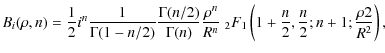
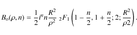
Since the Fourier transform of a sum is the sum of the Fourier transforms, the solution for a k sector mask reduces to the transform of vortex phase masks, a question treated by Mawet et al. (2005b). The problem in its general form is to find the Fourier transform of an Airy pattern distorted by a phase term , where n is an integer. According to Mawet et al. (2005b), the amplitude at the pupil plane image can be written as

where we have multiplied the amplitude with the area of the aperture for normalization, suppressed a multiplicative term -i irrelevant to the present study, and explicitly written the result as a separate function of and .

The amplitude in the re-imaged aperture plane takes a different form inside or outside the aperture. We give thereafter the expressions C7 of Mawet et al. (2005b) after correction of a few typos. Inside the aperture, takes the form

where is the hypergeometric function, and is identically zero for even values of n since equals zero for 0 and negative integer arguments. This property demonstrates the null inside the aperture image for sector masks of order k for which (2 m + 1) k/2 is an even number. Since m can take the value of 0, k/2 must be an even number and the efficient masks must be multiples of 4. This is therefore a more general demonstration of what is given in Appendix A.

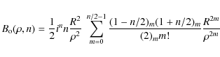
Outside the aperture image, can be written as

A simplification of the hypergeometric function can be made because of the particular values of its first argument. For n=2, the function equals 1. For n=4 and higher even integer, the first argument is a negative integer. The hypergeometric function reduces to a polynomial of n/2 terms (see Abramowitz & Stegun 1972, p. 561):

where (a)_m is the Pochhammer symbol equal to . This expression can be further simplified to

where is the radial Zernike polynomial Z_n^m(r) normalized so that Z_n^m(1)=1. The use of the Zernike polynomial instead of the hypergeometric function ensures that the numerical evaluation is faster and more precise. Note that the Zernike polynomials apply to the complex amplitude of the wave, not to the phase (see Ferrari 2007). For example, the first three terms for n equal to 2, 4, and 6 can be written as

One can verify that for any even value of n the light rejected outside the aperture image exactly equals the incoming flux through the aperture. This can be achieved by integrating the intensity diffracted outside the aperture. Because it is a radial function, we can write

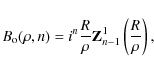
We return to the 4Q and 8O phase masks. The diffracted amplitude of a mask of k sectors in the pupil plane can be evaluated by substituting the effects of the phase terms in the Fourier series expression of the mask. We have

with , where the sine function originates in the composition of the two complex exponential terms. The use of Zernike polynomials makes it possible to compute using a much larger number of terms than with the otherwise diverging hypergeometric function.

We can verify that the light rejected outside the aperture still equals the incoming flux in the aperture. This can be achieved by summing for varying from R to and varying from 0 to 2. The modulus squared of the sum can be expressed as a double sum. Because of the orthogonality property of the sine function, cross terms with different values cancel after the angular integration. The computation reduces to a simple sum that can be easily computed using the above results for a single vortex. We have

In practice, we limit the number of terms in the theoretical expression of . A sum of 10 terms will recover 98 of the flux, and 20 terms 99.

It may be of interest to consider the case of the phase knife (k=2) to quantify the effect of the mask on the planet when it lies exactly over two sectors, sufficiently away from the center to neglect the effect of the other sectors. The phase coefficients correspond to a vortex of odd charges (1+2m) and there is a null no more inside the aperture image. The function of Eq. (B.3) must then be expressed at -1/2, -3/2, etc, hopefully close to a local maximum. The basic expressions with the hypergeometric functions remain valid, but not the simplifications.

Illustrations for the amplitude diffracted by various sector masks (k=2, 4, 8 and 12) are given in Fig. B.1. For the 4, 8, and 12 sectors, the mask transmissions are even functions, andthe amplitude is real, symmetric, and alternatively positive and negative around the diffraction pattern. For the phase knife, the amplitude is imaginary and anti-symmetric. The complexity of the images increases with the number of sectors in successive rings. As already experimentally observed, the spread of the pattern increases with k.

In Fig. B.2 we give the normalized intensity flux left by a phase mask for a Lyot stop of variable diameter. For a 4QC or an 8OC, this indicates the level of the light for a planet crossing exactly the border that divides two quadrants. Our Lyot stop has a diameter that is 93% of the pupil diameter, and theoretically induces an attenuation that is approximately equal to 0.16 times the original intensity. In practice the measured attenuation is 0.2 which can be explained by a slight misalignment of the PSF's center over the axes. For a perfect instrument, a Lyot stop exactly equal to the aperture, 2/3 of the light is lost when a faint companion crosses exactly a sector of the mask far from the center. This corresponds to a loss of about 1.2 mag, which is much less than generally expected (Rouan et al. 2007).

References

• Abe, L., Vakili, F., & Boccaletti, A. 2001, A&A, 374, 1161 [NASA ADS] [CrossRef] [EDP Sciences] (In the text)
• Abe, L., Domiciano de Souza, Jr., A., Vakili, F., & Gay, J. 2003, A&A, 400, 385 [NASA ADS] [CrossRef] [EDP Sciences] (In the text)
• Abe, L., Beaulieu, M., Vakili, F., et al. 2007, A&A, 461, 365 [NASA ADS] [CrossRef] [EDP Sciences] (In the text)
• Abramowitz, M., & Stegun, I. A. 1972, Handbook of Mathematical Functions (New York: Dover) (In the text)
• Aime, C., Carlotti, A., & Ricort, G. 2007, Comptes Rendus Physique, 8, 961 [NASA ADS] [CrossRef] (In the text)
• Carlotti, A., Ricort, G., Aime, C., El Azhari, Y., & Soummer, R. 2008, A&A, 477, 329 [NASA ADS] [CrossRef] [EDP Sciences] (In the text)
• Ferrari, A. 2007, ApJ, 657, 1201 [NASA ADS] [CrossRef] (In the text)
• Gay, J. 2002, private communication (In the text)
• Jenkins, C. 2008, MNRAS, 384, 515 [NASA ADS] [CrossRef] (In the text)
• Lloyd, J. P., Gavel, D. T., Graham, J. R., et al. 2003, in SPIE Conf. Ser. 4860, ed. A. B. Schultz, 171 (In the text)
• Mawet, D., Riaud, P., Absil, O., Baudrand, J., & Surdej, J. 2005a, in SPIE Conf. Ser. 5905, ed. D. R. Coulter, 502
• Mawet, D., Riaud, P., Absil, O., & Surdej, J. 2005b, ApJ, 633, 1191 [NASA ADS] [CrossRef] (In the text)
• Murakami, N., Uemura, R., Baba, N., et al. 2008, PASP, 120, 1112 [NASA ADS] [CrossRef] (In the text)
• Riaud, P., Boccaletti, A., Rouan, D., Lemarquis, F., & Labeyrie, A. 2001, PASP, 113, 1145 [NASA ADS] [CrossRef] (In the text)
• Rouan, D., Riaud, P., Boccaletti, A., Clénet, Y., & Labeyrie, A. 2000, PASP, 112, 1479 [NASA ADS] [CrossRef] (In the text)
• Rouan, D., Baudrand, J., Boccaletti, A., et al. 2007, Comptes Rendus Physique, 8, 298 [NASA ADS] [CrossRef] (In the text)

Footnotes

... form

Another way of achieving this result is to express the mask directly in polar coordinates, as indicated to us by the anonymous referee.

All Figures

---

Copyright ESO 2009