| Issue |
A&A
Volume 504, Number 2, September III 2009
|
|
|---|---|---|
| Page(s) | 681 - 688 | |
| Section | Catalogs and data | |
| DOI | https://doi.org/10.1051/0004-6361/200911979 | |
| Published online | 09 July 2009 | |
Integrated BVJHK parameters and luminosity functions
of 650 Galactic open clusters
parameters and luminosity functions
of 650 Galactic open clusters![[*]](/icons/foot_motif.png)
N. V. Kharchenko1,2,3 - A. E. Piskunov1,3,4 - S. Röser3 - E. Schilbach3 - R.-D. Scholz1 - H. Zinnecker1
1 - Astrophysikalisches Institut Potsdam, An der Sternwarte 16,
14482 Potsdam, Germany
2 -
Main Astronomical Observatory, 27 Academica Zabolotnogo Str., 03680
Kiev, Ukraine
3 -
Astronomisches Rechen-Institut, Mönchhofstraße 12-14,
69120 Heidelberg, Germany
4 -
Institute of Astronomy of the Russian Acad. Sci., 48 Pyatnitskaya
Str., 109017 Moscow, Russia
Received 3 March 2009 / Accepted 20 May 2009
Abstract
Aims. We determine the integrated magnitudes and colours of 650 clusters in optical (BV) and the near-infrared (
![]() )
passbands and construct the luminosity functions of the Galactic open clusters in these passbands.
)
passbands and construct the luminosity functions of the Galactic open clusters in these passbands.
Methods. The magnitudes are based on accurate and uniform cluster membership parameters derived from the ASCC-2.5 catalogue and were computed by adding the individual luminosities of the most secure cluster members. To put the computed magnitudes into a uniform and unbiased system, they were corrected for the effect of unseen stars in the ASCC-2.5. Comparison of the derived parameters with published optical data shows that our integrated magnitudes and colours are accurate within 0.6 and 0.2 mag, respectively. Comparison of cluster distributions over apparent integrated magnitudes with the prediction of a model of cluster counts shows that the sample can be regarded as magnitude-limited down to 8.1, 7.7, 6.3, 5.3, and 5.3 mag in
![]() .
.
Results. Out of 650 clusters, 422 (or about 2/3) have received optical integrated magnitudes for the first time. This increases the data bank of BV integrated magnitudes to about 780 clusters, compared to about 350 clusters with BV-magnitudes available in the literature. In the near-infrared, data on cluster-integrated parameters were not available before this study. The cluster sample is found to be magnitude-limited both in the optical and in the near-infrared. This enabled us to construct cluster luminosity functions in five (
![]() )
photometric passbands. We find that both in the optical and in the NIR the luminosity functions show similar behaviour: a linear increase to fainter magnitudes, which stops at about -2.5 mag in the optical and at -4.0 mag in the NIR. At the brightest magnitudes the luminosity functions exhibit a deficiency with respect to the linear relation. The youngest clusters have flatter luminosity functions in all five passbands with a slope of about 0.2-0.3, while the total cluster sample (all ages) produces luminosity functions with significantly steeper slopes of the order of
0.35-0.50.
)
photometric passbands. We find that both in the optical and in the NIR the luminosity functions show similar behaviour: a linear increase to fainter magnitudes, which stops at about -2.5 mag in the optical and at -4.0 mag in the NIR. At the brightest magnitudes the luminosity functions exhibit a deficiency with respect to the linear relation. The youngest clusters have flatter luminosity functions in all five passbands with a slope of about 0.2-0.3, while the total cluster sample (all ages) produces luminosity functions with significantly steeper slopes of the order of
0.35-0.50.
Key words: Galaxy: evolution - Galaxy: open clusters and associations: general - solar neighbourhood - Galaxy: stellar content
1 Introduction
Our current project studies the properties of the local population
of Galactic or Milky Way (MW) open clusters. The sample contains 650 open clusters and compact
associations identified in the all-sky compiled catalogue of 2.5 million
stars, ASCC-2.5 (Kharchenko 2001). For each cluster, we determined combined spatial
kinematical-photometric membership (Kharchenko et al. 2004) and derived a
homogeneous set of cluster parameters (Kharchenko et al. 2005a,b). In a recent
study of Piskunov et al. (2008, Paper I hereafter) the integrated magnitudes of open
clusters in the V band were determined and used to construct cluster
luminosity and mass functions (CLF and CMF hereafter). In the present paper
we extend this study to other passbands
and discuss, in detail, different issues related to integrated magnitudes
and colours of local clusters in five passbands
![]() .
.
In contrast to e.g. cluster masses, integrated photometric parameters of star clusters can be obtained from observations directly. For extragalactic studies in particular, integrated magnitudes and colours provide the basis for constructing the cluster luminosity function with the subsequent conversion to the cluster mass function, as well as for determining the cluster age distribution with implications for the history of star formation and other issues related to studies of extragalactic populations. To obtain unbiased results all over the sky, one has to work in well-defined and uniform photometric systems. Although the Lund catalogue (Lyngå 1988) provides apparent integrated parameters for about 590 MW open clusters, no description of the input data and/or method is given, neither in the catalogue nor elsewhere. Therefore, these data can hardly be used as ``benchmarks'' for calibration purposes.
The pioneering work that determines the integrated colours and magnitudes of MW open clusters by Gray (1965) made use of UBV photometric data taken from the literature and resulted in integrated magnitudes I(MV) and colours I(B-V)0, I(U-B)0 of 67 open clusters. Gray (1965) implemented the method of summing up individual stellar luminosities with an extrapolation beyond the observation limit. Although no information on cluster membership was considered, the results from Gray (1965) are still widely used. In later determinations of integrated parameters for open clusters, attempts were made to take membership information into account. Piskunov (1974) derived integrated parameters of 22 open clusters with cluster members safely selected with respect to their proper motions and/or photometric data. Sagar et al. (1983) obtained integrated magnitudes I(MV) and colours I(B-V)0, I(U-B)0 for 142 open clusters (including the 22 clusters from Piskunov 1974). The cluster membership was based either on proper motions or on UBV photometry taken from the literature. Considering kinematic cluster members (proper motions or radial velocities), Spassova & Baev (1985) computed integrated UBV parameters of 50 open clusters. Pandey et al. (1989) extended the Sagar et al. (1983) sample by another 79 objects. Battinelli et al. (1994) published integrated magnitudes I(MV) and colours I(B-V)0, I(U-B)0 for 138 open clusters with available photometric membership, which, for a number of clusters, could be improved by kinematic constraints. Recently, Lata et al. (2002) updated the pool of published integrated parameters by data on 212 MW open clusters with CCD or photoelectric photometry available from the literature. For all clusters, I(MV) magnitudes and I(B-V)0 colours were determined, whereas I(U-V)0, I(V-R)0, I(V-I)0 could only be obtained for 15-60% of the clusters. For the membership determination, Lata et al. (2002) used photometric constraints. According to Lata et al. (2002), integrated parameters in the optical, I(MV) and I(B-V)0, are available for about 350 open clusters of the Milky Way. However, the data are strongly inhomogeneous since the photometric observations of different clusters were obtained with different instruments and detectors, and the data reduction was carried out with different methods by different authors. Frequently, the integrated magnitudes and colours were only ``by-products'' of studies aiming primarily at constructing photometric sequences (e.g., sets of photometric standards, or cluster CMDs), where the data completeness is not essential.
From this point of view, our data on the local open clusters are well-suited
to deriving a homogeneous set of integrated photometric parameters based on
uniform BV-photometry and membership information for all 650 clusters
identified in the ASCC-2.5 catalogue. Moreover, in the course of the preparation
of the PPMX catalogue (Röser et al. 2008), the ASCC-2.5 was cross-identified with
the 2MASS catalogue (Skrutskie et al. 2006). This offered the possibility to compute
reliable integrated parameters in five passbands
![]() for all clusters
from the sample and thus to construct luminosity functions of the Galactic
clusters in the five passbands.
for all clusters
from the sample and thus to construct luminosity functions of the Galactic
clusters in the five passbands.
We present in this paper the integrated magnitudes of 650 clusters computed both in the optical and near-infrared passbands. The magnitudes are corrected for unseen stars and compared with previous determinations. Using these data we construct luminosity functions of the MW open clusters and consider their evolution.
The paper has the following structure. Section 2 describes the cluster sample and the cluster data. We explain the method of determination of cluster integrated parameters and present the results in Sect. 3. The luminosity functions of open clusters are determined in the optical and near-infrared in Sect. 4. We summarise the results in Sect. 5.
2 Data
A reliable estimate of the integrated photometric parameters of open clusters requires proper information on cluster membership and homogeneous photometric measurements for cluster members. For each of the 650 clusters identified in the ASCC-2.5 (Kharchenko 2001), the membership of stars projected on the cluster area was determined in an iterative process, by taking into account their spatial (projected density profile), photometric (colour magnitude diagram, CMD), and proper motion (vector point diagram, VPD) distributions (Kharchenko et al. 2004). We express the cluster membership in terms of probabilities that are calculated from the location of the star in the VPD and CMD relative to the mean proper motions of the cluster and the cluster main sequence enhanced by the sequence of unresolved binaries. Stars deviating from the reference loci, both in the VPD and CMD, by less than one mean error have membership probabilities higher than 61%, and we classified them as the most probable members. Other stars with lower membership probabilities but higher than 14% and 1% are called possible cluster members and possible field stars, respectively. The data on the most probable members are used to derive cluster parameters such as the coordinates of the cluster centre, the cluster size, the mean proper motion, the distance from the Sun, reddening, and age. The results for 650 clusters are included in the Catalogue of Open Cluster Data (COCD) and its extension (Kharchenko et al. 2005a,b).
All cluster members have B, V magnitudes in the Johnson photometric
system taken from the ASCC-2.5, as well as J, H, ![]() from the 2MASS.
Therefore, homogeneous integrated parameters of open clusters can be derived
in five passbands.
from the 2MASS.
Therefore, homogeneous integrated parameters of open clusters can be derived
in five passbands.
3 Determination of integrated parameters
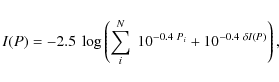
We define apparent I(P) and absolute I(MP) integrated magnitudes of a
cluster in a photometric passband P (with P corresponding to B, V,
J, H, or ![]() )
as
)
as
and
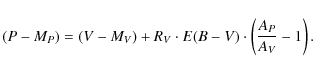
Here, N is the number of the most probable cluster members, Pi are their apparent magnitudes, and (P-MP) is the apparent distance modulus of a cluster in the passband P. The term
The parameters of interstellar extinction are taken from Cardelli et al. (1989) where the ratio RV of the total to selective extinction in optical is determined as RV = AV/E(B-V) = 3.1, and AB = 1.323 AV. For the near-infrared passbands, Cardelli et al. (1989) give AJ = 0.282 AV, AH = 0.190 AV, and AK = 0.114 AV. To convert K-magnitudes to the 2MASS passband
Following Gray (1965), integrated magnitudes I(MP) are usually computed from the sum of individual stellar luminosities, starting from the brightest star and extending to fainter stars over 4 or 5 mag. The integrated magnitude/luminosity is assumed to be the asymptotic value of the sum estimated either by extrapolation of a relationship I(P) vs. P for each cluster (Gray 1965), or by use of a cluster luminosity function (Tarrab 1982).
We computed corrections
![]() in a similar way as we did to obtain
the corrections
in a similar way as we did to obtain
the corrections
![]() in Paper I. The approach is based on
analysing the dependence I(MP) vs.
in Paper I. The approach is based on
analysing the dependence I(MP) vs. ![]() where
where ![]() is the
magnitude difference between a cluster member and the brightest cluster
stars; i.e. we considered the increase in the integrated brightness when
including fainter and fainter stars. Among the clusters with a sufficiently
wide magnitude range represented in the ASCC-2.5, we selected 27 ``template''
clusters listed in Table 1. The goal was to have 10 ``template''
clusters per photometric band with the brightest cluster stars covering a
wide range of absolute magnitudes MP. In Fig. 1 we show the
increase in the integrated absolute magnitude I(MP) as a function of
is the
magnitude difference between a cluster member and the brightest cluster
stars; i.e. we considered the increase in the integrated brightness when
including fainter and fainter stars. Among the clusters with a sufficiently
wide magnitude range represented in the ASCC-2.5, we selected 27 ``template''
clusters listed in Table 1. The goal was to have 10 ``template''
clusters per photometric band with the brightest cluster stars covering a
wide range of absolute magnitudes MP. In Fig. 1 we show the
increase in the integrated absolute magnitude I(MP) as a function of
![]() .
At
.
At
![]() ,
the integrated magnitude I(MP) is identical
to the absolute magnitude of the brightest member of the template cluster,
i.e.
,
the integrated magnitude I(MP) is identical
to the absolute magnitude of the brightest member of the template cluster,
i.e.
![]() .
Although
``template'' clusters show a different behaviour at small
.
Although
``template'' clusters show a different behaviour at small ![]() ,
the integrated absolute magnitudes I(MP) stop the increasing in almost all ``template'' clusters
at
,
the integrated absolute magnitudes I(MP) stop the increasing in almost all ``template'' clusters
at
![]() .
Therefore, we chose
.
Therefore, we chose
![]() to be the reference
value for the determination of corrections
to be the reference
value for the determination of corrections
![]() .
.
Table 1: The ``template'' cluster list.
![\begin{figure}
\par\includegraphics[angle=-90,width=9cm,clip]{11979fg1.eps}
\end{figure}](/articles/aa/full_html/2009/35/aa11979-09/img28.png) |
Figure 1:
Absolute integrated magnitude I(MP) profiles for ``template''
clusters in different passbands (10 ``templates'' for each band). The
vertical bars indicate individual cluster members. The COCD numbers are
shown at each profile. The vertical dotted lines separate stars fainter
than
|
| Open with DEXTER | |
For each cluster with an observed magnitude range less than 7 mag in the
ASCC-2.5, the corrections
![]() were computed as
were computed as
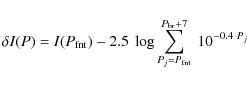
where
| |
Figure 2:
The distributions of
|
| Open with DEXTER | |
The template profiles in Fig. 1 show different behaviours of integrated magnitudes for different clusters. They correlate mainly with the cluster age and the relation of the magnitude of the brightest member to the magnitudes of fainter cluster stars. In a young open cluster where O- or B-stars are still observed, the integrated magnitude is usually dominated by the brightest member, and the corresponding profile is flat. In an older cluster the magnitude difference between the brightest member and the next members (e.g., the second brightest member) is less prominent, and the corresponding profile can show considerable increment. However, even in this case, the total contribution of the fainter stars to the integrated magnitude seldom exceeds 2 mag (see Fig. 2).
![\begin{figure}
\par\includegraphics[angle=-90,width=9cm,clip]{11979fg3.eps}
\end{figure}](/articles/aa/full_html/2009/35/aa11979-09/img38.png) |
Figure 3:
The difference of integrated magnitudes for two membership samples
of ASCC-2.5 clusters (the standard selection [PM, ph], and photometric-only [ph]
selection) vs. I(V). The blue dashed line indicates the mean difference
between the data: +0.88 mag with st.dev. |
| Open with DEXTER | |
The resulting integrated parameters depend on the reliability of the membership determination. This effect is illustrated by Fig. 3 where we compare integrated magnitudes in V computed with members selected by different constraints. In the first case, we take the most probable members according to the combined spatio-photometric-kinematic criteria (i.e., our standard approach); in the second case, we consider the results of the spatio-photometric selection alone. The average differences in the integrated parameters are given in Table 2 (first line). Neglecting the kinematic constraints causes a higher contamination of stellar samples by field stars. This results in a systematic underestimation of integrated magnitudes making clusters, on average, about 1 mag brighter. For several clusters, the discrepancy is considerably greater due to the inclusion of relatively bright foreground stars with different kinematics from the corresponding cluster proper motions.
In Fig. 4 we compare our data on I(MV) and I(B-V)0 with integrated parameters of the galactic open clusters published by Lata et al. (2002, 73 clusters in common) and Battinelli et al. (1994, 96 clusters in common). The integrated parameters in Lata et al. (2002) are based on stars with photometric membership. Battinelli et al. (1994) note that, wherever possible, they applied proper motion criteria in addition to photometric constraints for their membership selection. The averaged differences between the published and our data are shown in Table 2. Again, we compared both of our sets of integrated parameters derived as described above. For the case of the standard membership selection, our magnitudes are fainter by about 0.5 mag. A possible explanation is that photometric constraints are not sufficient to remove bright foreground stars from the samples of Lata et al. (2002) and Battinelli et al. (1994), and kinematic data based on pre-Hipparcos proper motions are instead too incomplete and inaccurate to improve the membership determination. However, for the case of purely photometric membership, our integrated magnitudes are somewhat brighter. The difference may arise from the different cluster parameters used (e.g., distance modulus) or different photometric constraints for determining membership (e.g., based on different isochrones).
![\begin{figure}
\par\includegraphics[angle=-90,width=9cm,clip]{11979fg4.eps}
\end{figure}](/articles/aa/full_html/2009/35/aa11979-09/img39.png) |
Figure 4: Difference in integrated parameters between previous determinations and this paper. The upper panels are for colours, the bottom panels for magnitudes. Left panels: ASCC-2.5 sample with standard membership based on kinematic and photometric criteria; right panels: ASCC-2.5 sample with photometry-only membership. The black crosses mark differences between our data and Lata et al. (2002), the red open circles show differences between this paper and Battinelli et al. (1994). The blue dashed lines indicate the average differences. |
| Open with DEXTER | |
Table 2: The average differences of integrated photometric parameters derived with different membership criteria.
After correcting for the systematic differences, the published data were used
to estimate the accuracy of our integrated magnitudes I(MV) and colours
I(B-V)0. Assuming that the random errors in the data by Lata et al. (2002)
and Battinelli et al. (1994) are approximately the same, we found that our I(MV)and I(B-V)0 are accurate within ![]() mag and
mag and ![]() mag,
respectively. Both values are rms-errors drawn from the comparison
with published data after excluding the systematic differences.
The uncertainty coincides with estimates of
mag,
respectively. Both values are rms-errors drawn from the comparison
with published data after excluding the systematic differences.
The uncertainty coincides with estimates of ![]() mag
and
mag
and ![]() mag reported by Sagar et al. (1983), who analysed uncertainties
introduced by different parameters participating in the determination of the
integrated magnitudes (photometry, reddening, distance modulus, etc.).
mag reported by Sagar et al. (1983), who analysed uncertainties
introduced by different parameters participating in the determination of the
integrated magnitudes (photometry, reddening, distance modulus, etc.).
Our determined integrated magnitudes and distance moduli in
![]() of 650 clusters are available in electronic form only at the CDS Strasbourg.
of 650 clusters are available in electronic form only at the CDS Strasbourg.
| |
Figure 5:
Distributions of apparent integrated magnitudes for the
|
| Open with DEXTER | |
4 Luminosity functions of open clusters in the optical and near-infrared
In Paper I we have already computed the cluster luminosity
function based on the integrated magnitudes in the V passband. Since
we have now integrated magnitudes in five passbands for all clusters of our
sample, it is reasonable to repeat the calculations for all
![]() magnitudes and compare the cluster luminosity functions derived in different
passbands. For the construction of the CLFs, we implement the technique
developed in Paper I. Like in Paper I, we
consider two young clusters, NGC 869 (h Per) and NGC 884 (
magnitudes and compare the cluster luminosity functions derived in different
passbands. For the construction of the CLFs, we implement the technique
developed in Paper I. Like in Paper I, we
consider two young clusters, NGC 869 (h Per) and NGC 884 (![]() Per), as a
single entity for the following reasons. The clusters are overlapping in the
projection on the sky, share a huge corona, and have a large number (more
than 50%) of members in common, making accurate determination of their
individual integrated photometric indices rather difficult. Also, we exclude
the cluster Mamajek 1 (
Per), as a
single entity for the following reasons. The clusters are overlapping in the
projection on the sky, share a huge corona, and have a large number (more
than 50%) of members in common, making accurate determination of their
individual integrated photometric indices rather difficult. Also, we exclude
the cluster Mamajek 1 (![]() Chamaeleontis) for which we could only
identify three members in the ASCC-2.5. According to Paper I, this
cluster can be omitted without consequences for the results. Therefore, our
final cluster sample includes 648 entities.
Chamaeleontis) for which we could only
identify three members in the ASCC-2.5. According to Paper I, this
cluster can be omitted without consequences for the results. Therefore, our
final cluster sample includes 648 entities.
First of all we examine whether our sample can be regarded as a magnitude-limited
one, which is complete up to a certain ``completeness'' magnitude
![]() .
The issue of completeness plays a key role in the construction of the
luminosity function. Throughout our study of the MW open cluster
population, we approached this problem from different angles. In
Piskunov et al. (2006), based on the analysis of the spatial distribution of clusters,
we showed that the sample is complete in the solar neighbourhood within a
distance of 850 pc. Later (in Paper I) we found that it can also be regarded
as complete down to the integrated apparent magnitude
.
The issue of completeness plays a key role in the construction of the
luminosity function. Throughout our study of the MW open cluster
population, we approached this problem from different angles. In
Piskunov et al. (2006), based on the analysis of the spatial distribution of clusters,
we showed that the sample is complete in the solar neighbourhood within a
distance of 850 pc. Later (in Paper I) we found that it can also be regarded
as complete down to the integrated apparent magnitude
![]() .
This enabled us to apply a technique suitable to a magnitude-limited sample
for the CLF/CMF determination.
.
This enabled us to apply a technique suitable to a magnitude-limited sample
for the CLF/CMF determination.
In the present study, extending the CLF to other passbands, we also extend our completeness analysis. Instead of the linear approach used in Paper I (valid for the idealised case of a uniform spatial distribution of the objects), we adopt here a model of cluster counts, for which the simplified assumptions on cluster spatial distribution are no longer necessary. We rely on a model developed by Kharchenko & Schilbach (1996) and on the data on the local cluster population derived in Piskunov et al. (2006).
The theoretical distribution reproducing the number of star clusters
N(I1,I2)![]() observed over the sky and having
apparent integrated magnitudes in the range [I1,I2] is computed along with
the first fundamental equation of stellar statistics:
observed over the sky and having
apparent integrated magnitudes in the range [I1,I2] is computed along with
the first fundamental equation of stellar statistics:
![\begin{displaymath}N(I_1,I_2)= \int\limits_{I_1}^{I_2}\iint\limits_{(4~\pi)}^{}
...
...\vec{\rho})~\varphi[I(M)]~R^2~{\rm d}R~{\rm d}\omega~{\rm d}I,
\end{displaymath}](/articles/aa/full_html/2009/35/aa11979-09/img58.png)
where the integration is carried out over the apparent magnitude range, and over the volume of the Milky Way. Here,
The CLF is a priori unknown and has to be determined either directly from the above integral equation or via an iterative procedure. We used the latter approach, with the initial approximation taken from the linear treatment implemented in Paper I. The details of the CLF construction are given below. At any iteration we used the CLF derived in the previous step, constructed the theoretical distribution, and derived a new value of the completeness limit from the comparison of modelled and observed distributions. The limit was set as a magnitude where the disagreement between the theoretical and observed distributions systematically exceeds one Poisson error. This new value is used in calculating the next approximation of the CLF. The iterations were continued until the completeness limit did not change. Three iterations were sufficient to reach convergence.
Table 3:
Parameters of cluster luminosity functions in
![]() passbands.
passbands.
Since the open clusters of our sample represent a single population
belonging to the thin disk, we adopted the following relation for
![]() (Bahcall & Soneira 1980):
(Bahcall & Soneira 1980):
where r and z are the projections of the vector
Interstellar extinction was taken into account according to the so-called Parenago
law (Parenago 1940) smoothly reproducing the large-scale structure of the Galactic dust layer:
![\begin{displaymath}A_P=\frac {a_P \cdot h_{a}}{\vert\sin b\vert}
\cdot \left[1 -...
...\{\frac {-R \cdot \vert\sin b\vert}{h_{a}}\right\}\right]\cdot
\end{displaymath}](/articles/aa/full_html/2009/35/aa11979-09/img100.png)
We assumed the scale height of an extinction layer to be ha=100 pc. The specific extinction in V is computed as the average over the cluster sample and found to be equal to aV = 0.7 mag/kpc. For the other passbands, the specific extinctions aP were recomputed from aV along with the Cardelli et al. (1989) relations (see Sect. 3).
The completeness magnitudes ![]() and the number of clusters with
and the number of clusters with
![]() for the B,V,J,H, and
for the B,V,J,H, and ![]() passbands are indicated in the two
upper lines of Table 3. The theoretical distributions for all the passbands are shown
with the observed histograms in Fig. 5. We note the good agreement of both types of distributions coinciding within one Poisson error at brighter magnitudes. This means that the
model adequately describes the observations to a certain magnitude limit. Beyond
this limiti, the degree of the disagreement drastically increases with stellar
magnitude. We attribute this behaviour to cluster sample incompleteness that
increases with increasing average cluster distance. Comparing the observed and predicted numbers of clusters, we can conclude that, at the magnitude limits chosen, the samples are complete to about 99%. This finding agrees with our previous conclusions on the spatial and magnitude-limited completeness of our sample. Although the theoretical distributions show a certain
degree of nonlinearity, they do not deviate strongly from linear behaviour
in the considered range of apparent magnitudes. This indicates that the results
on the local CLF derived in Paper I do not differ strongly from the present
findings.
passbands are indicated in the two
upper lines of Table 3. The theoretical distributions for all the passbands are shown
with the observed histograms in Fig. 5. We note the good agreement of both types of distributions coinciding within one Poisson error at brighter magnitudes. This means that the
model adequately describes the observations to a certain magnitude limit. Beyond
this limiti, the degree of the disagreement drastically increases with stellar
magnitude. We attribute this behaviour to cluster sample incompleteness that
increases with increasing average cluster distance. Comparing the observed and predicted numbers of clusters, we can conclude that, at the magnitude limits chosen, the samples are complete to about 99%. This finding agrees with our previous conclusions on the spatial and magnitude-limited completeness of our sample. Although the theoretical distributions show a certain
degree of nonlinearity, they do not deviate strongly from linear behaviour
in the considered range of apparent magnitudes. This indicates that the results
on the local CLF derived in Paper I do not differ strongly from the present
findings.
In spite of the general agreement between theoretical and observed
distributions, one notes some enhancement of the observed histogram with
respect to the modelled curve, better seen in the shorter wavelength histograms. We
relate this enhancement to a real density fluctuation corresponding to Gould's
Belt clusters (see Piskunov et al. 2006). One can also see that the ``depth'' of
the sample (which we define as the fraction of clusters above the completeness
limit) is lowering towards longer wavelengths. This is a natural consequence of
a change in cluster brightness from the B to the ![]() passband. Indeed, on average the optical clusters containing OB stars are intrinsically brighter than those with red giants (RG), and vice versa in the NIR. Then, in a sample constructed on the basis of an optical survey (our case), the average observed location of RG-clusters is closer to the Sun than those of OB-clusters. When one sorts the clusters of such a sample along with their NIR-magnitudes one finds at the top closer and apparently brighter clusters, which also provide a brighter apparent completeness limit.
passband. Indeed, on average the optical clusters containing OB stars are intrinsically brighter than those with red giants (RG), and vice versa in the NIR. Then, in a sample constructed on the basis of an optical survey (our case), the average observed location of RG-clusters is closer to the Sun than those of OB-clusters. When one sorts the clusters of such a sample along with their NIR-magnitudes one finds at the top closer and apparently brighter clusters, which also provide a brighter apparent completeness limit.
In the following analysis we only consider clusters apparently brighter
than the completeness magnitudes
![]() in each passband. As the CLFs are
constructed from the above clusters, they can be considered free of
sample-incompleteness biases.
in each passband. As the CLFs are
constructed from the above clusters, they can be considered free of
sample-incompleteness biases.
For every jth cluster of such a subsample, one can determine a radius
of the completeness circle ![]() ,
which only depends on the completeness limit
,
which only depends on the completeness limit
![]() ,
the cluster absolute magnitude Ij(MP), and the interstellar
extinction AP,j on the way to the cluster:
,
the cluster absolute magnitude Ij(MP), and the interstellar
extinction AP,j on the way to the cluster:
![\begin{displaymath}\log \hat{d}_j = 0.2~[\hat{I}_P - I_j(M_P) - A_{P,j}] + 1.
\end{displaymath}](/articles/aa/full_html/2009/35/aa11979-09/img104.png)
We use here a subscript j to emphasise the individual character of the derived limiting distance. With these parameters the cluster gives its individual contribution (a partial density) to the local surface density, which can be computed as
The following is straightforward. The cluster luminosity function
![]() is constructed as the sum of partial densities of clusters with absolute
integrated magnitudes in the range
is constructed as the sum of partial densities of clusters with absolute
integrated magnitudes in the range
![]() where
where
![]() is a bin of the distribution
is a bin of the distribution
![\begin{displaymath}\phi[I_i(M_P)] =\frac{1}{\Delta
I(M_P)}\sum\limits_j^{n_i}\frac{1}{\pi~{\hat{d}_j}^{~2}}\cdot
\end{displaymath}](/articles/aa/full_html/2009/35/aa11979-09/img109.png)
Here, ni is the number of clusters in the ith magnitude bin Ii(MP), and
![\begin{figure}
\par\includegraphics[origin=rb,angle=-90,width=11.5cm,clip]{11979fg6.eps}
\end{figure}](/articles/aa/full_html/2009/35/aa11979-09/img111.png) |
Figure 6:
Luminosity functions of the MW open clusters in different
photometric passbands for three cluster samples that differ by the upper
limit of the age of the included clusters. The upper (black) curves show the
total sample corresponding to the CPDLF, the middle (magenta) curves are for
moderately young clusters (
|
| Open with DEXTER | |
In Fig. 6 we show the CLFs for the passbands
![]() constructed under the assumption that their completeness limits correspond
to the values from Table 3. In Fig. 6 we consider
three cluster subsamples with different upper limits of cluster ages. The
first subsample represents clusters of all ages (
constructed under the assumption that their completeness limits correspond
to the values from Table 3. In Fig. 6 we consider
three cluster subsamples with different upper limits of cluster ages. The
first subsample represents clusters of all ages (
![]() )
and the corresponding CLFs
can be considered to be the present-day luminosity functions of clusters
(CPDLF). The second subsample comprises only young clusters with
)
and the corresponding CLFs
can be considered to be the present-day luminosity functions of clusters
(CPDLF). The second subsample comprises only young clusters with
![]() .
This subsample can be associated with the initial luminosity
function of clusters (CILF). The third subsample comprises intermediate-age
young clusters with
.
This subsample can be associated with the initial luminosity
function of clusters (CILF). The third subsample comprises intermediate-age
young clusters with
![]() and is given for comparison.
and is given for comparison.
The CLFs are binned to have 5 objects in each bin. One can see that all the
luminosity functions exhibit a similar general behaviour. The most common
feature, which can be found both at different ages and in different
passbands, is the linear increase in the CLF towards fainter magnitudes. The
CLFs change their slopes after they reach some magnitude, different in
various spectral domains. (In the optical the limit is at about -2.5 mag and
in the NIR it is at about -4.0 mag.) In our previous
work we attributed this change to evolutionary effects related to cluster
decay. The brighter portion of the CLF indicates a deficiency with respect to
the linear behaviour. We fitted the linear portion of the CLF by the
equation:
The details of the fit are given in Table 3.
As can be seen from Table 3, the slope p increases with increasing
upper limit of the sample age from ![]() 0.2...0.3 (clusters with
0.2...0.3 (clusters with
![]() )
to
)
to
![]() (clusters of
all ages). This steepening of the CLF is also observed in Fig. 6.
In order to get quantitative evidence for the evolution of the CLF slope, we
constructed the CLF slope-age relation for every passband, with the limiting age
of the sample varying from
(clusters of
all ages). This steepening of the CLF is also observed in Fig. 6.
In order to get quantitative evidence for the evolution of the CLF slope, we
constructed the CLF slope-age relation for every passband, with the limiting age
of the sample varying from
![]() to
to
![]() .
These relations are shown in Fig. 7.
.
These relations are shown in Fig. 7.
| |
Figure 7: The CLF slope p as a function of the upper limit of the age of the cluster sample in different photometric passbands. |
| Open with DEXTER | |
One should
note that the evolution of the slope is approximately the same in different
passbands (except for J, where the CLFs at different ages are steeper by about 0.1), and a certain difference of the relations at young ages (say
![]() )
should be attributed to the lower confidence of the slopes
for young subsamples because there are less sample members.
)
should be attributed to the lower confidence of the slopes
for young subsamples because there are less sample members.
The observed steepening of the CLF might be accounted for by cluster evolution. In fact, there are two concurrent processes responsible for a cluster appearance: physical evolution of cluster members (so-called ``fading'') and dynamical mass loss, resulting in a full decay (``cluster disruption''). Both have different time scales depending on cluster parameters. The rate of fading depends on cluster age, whereas the disruption time is a direct function of cluster mass. That is why, at the extremes of the magnitude range, the engines driving the CLF evolution are different. At the bright end, where young OB-clusters are concentrated, the fading effect plays the primary role. At the faint end, comprising mainly old and/or low-mass clusters, the evolution is driven basically by the disruption. Since an optical magnitude-limited sample favours OB (i.e. young) clusters, we consider the CLF steepening as a manifestation of their evolutionary fading coupled with the continuous formation of new clusters. Thus the CLF slope keeps information both on the cluster evolution and the cluster formation history in the Galactic disk.
The important immediate conclusion that follows from the relations is that the slope of the CPDLF is not equal to that of the CILF. The difference between the CILF and CLF already becomes substantial at
![]() ,
which is frequently regarded as the age of the very young cluster population. To avoid wrong conclusions on the underlying initial mass function of star clusters, one should take the evolutionary changes of the CLF into account.
,
which is frequently regarded as the age of the very young cluster population. To avoid wrong conclusions on the underlying initial mass function of star clusters, one should take the evolutionary changes of the CLF into account.
The tabulated data on the CLFs shown in Fig. 6 can be found in a table, which is only available in electronic form at the CDS Strasbourg.
5 Conclusions
Using data on accurate and homogeneous spatio-kinematic-photometric
membership for 650 MW open clusters, we have computed their integrated
magnitudes in the optical (BV) and the near-infrared (
![]() ). Compared
to previous lists of integrated magnitudes (e.g. those of Battinelli et al. 1994; Lata et al. 2002, and others
mentioned in Sect. 1) of Galactic star
clusters our data are based on independent, spatially unbiased, and uniform
data. This allows their use as benchmarks for model evolutionary
synthesis or for studies of the extragalactic populations of star clusters.
Out of 650 clusters with optical magnitudes derived in this study, 422 (or
about 2/3) received these values for the first time. Noting that in the
literature these values were known before for 352 clusters, this study
increases the data bank of BV integrated magnitudes to about 780 clusters,
or by more than a factor of two. In the near-infrared, data on clusters'
integrated magnitudes were not available before this study.
). Compared
to previous lists of integrated magnitudes (e.g. those of Battinelli et al. 1994; Lata et al. 2002, and others
mentioned in Sect. 1) of Galactic star
clusters our data are based on independent, spatially unbiased, and uniform
data. This allows their use as benchmarks for model evolutionary
synthesis or for studies of the extragalactic populations of star clusters.
Out of 650 clusters with optical magnitudes derived in this study, 422 (or
about 2/3) received these values for the first time. Noting that in the
literature these values were known before for 352 clusters, this study
increases the data bank of BV integrated magnitudes to about 780 clusters,
or by more than a factor of two. In the near-infrared, data on clusters'
integrated magnitudes were not available before this study.
The other important feature of the sample is the statistical independence of the data. All previous collections are based on various sources of ground-based photometry from the literature, while the present data come from the uniform all-sky photometry of the (space-borne) Tycho experiment. This enabled us to estimate the accuracy of the data by comparison with external data assuming that most extended published data collections (Battinelli et al. 1994; Lata et al. 2002) have statistically independent origins. From this we found that our integrated magnitudes and colours are accurate to 0.6 and 0.2 mag, respectively.
In this study we confirm that our data sample can be regarded as
magnitude-limited both in the optical and in the near-infrared. Applying the
technique of luminosity function construction in a magnitude-limited sample
proposed in our Paper I, we have determined here cluster
luminosity functions in five passbands (
![]() ). We find that both in
the optical and in the NIR the CLFs show qualitatively similar behaviour:
linear increase to fainter magnitudes, which slows down at about -2.5 mag
in the optical and -4.0 mag in the NIR. At the brightest magnitudes (
I(MP)
< -8 mag) the CLFs exhibit a certain deficiency with respect to the linear
relation.
). We find that both in
the optical and in the NIR the CLFs show qualitatively similar behaviour:
linear increase to fainter magnitudes, which slows down at about -2.5 mag
in the optical and -4.0 mag in the NIR. At the brightest magnitudes (
I(MP)
< -8 mag) the CLFs exhibit a certain deficiency with respect to the linear
relation.
We also find that the sample of the youngest clusters have flatter CLFs in
all five passbands examined. The typical slope of CLFs for clusters with
![]() ,
which could be regarded to be close to the CILF, is
0.2-0.3. When adding older clusters, one gets steeper CLFs. When clusters
of all ages presented in our samples are considered (
,
which could be regarded to be close to the CILF, is
0.2-0.3. When adding older clusters, one gets steeper CLFs. When clusters
of all ages presented in our samples are considered (
![]() ),
the CLFs (which correspond to the CPDLFs in this case) show a significantly steeper
slope of the order of 0.4-0.5. This difference can be noted already at
ages of
),
the CLFs (which correspond to the CPDLFs in this case) show a significantly steeper
slope of the order of 0.4-0.5. This difference can be noted already at
ages of
![]() .
Thus for a correct construction of
the cluster initial luminosity and/or mass function one needs to either
select objects younger than 100 Myr or take the evolutionary
steepening of the CLF into account.
.
Thus for a correct construction of
the cluster initial luminosity and/or mass function one needs to either
select objects younger than 100 Myr or take the evolutionary
steepening of the CLF into account.
Acknowledgements
This study was supported by DFG grant 436 RUS 113/757/0-2, and RFBR grant 07-02-91566. We acknowledge the useful comments by the anonymous referee.
References
- Bahcall, J. N., & Soneira, R. M. 1980, ApJS, 44, 73 [NASA ADS] [CrossRef] (In the text)
- Battinelli, P., Brandimarti, A., & Capuzzo-Dolcetta, R. 1994, A&AS, 104, 379 [NASA ADS] (In the text)
- Cardelli, J. A., Clayton, G. C., & Mathis, J. S. 1989, ApJ, 345, 245 [NASA ADS] [CrossRef] (In the text)
- Gray, D. F. 1965, AJ, 70, 362 [NASA ADS] [CrossRef] (In the text)
- Kharchenko, N., & Schilbach, E. 1996, Baltic Astron., 5, 337 [NASA ADS] (In the text)
- Kharchenko, N. V. 2001, Kinematics and Physics of Celestial Bodies, 17, 409 (In the text)
- Kharchenko, N. V., Piskunov, A. E., Röser, S., Schilbach, E., & Scholz, R.-D. 2004, Astron. Nachr., 325, 743 [NASA ADS] (In the text)
- Kharchenko, N. V., Piskunov, A. E., Röser, S., Schilbach, E., & Scholz, R.-D. 2005a, A&A, 438, 1163 [NASA ADS] [CrossRef] [EDP Sciences]
- Kharchenko, N. V., Piskunov, A. E., Röser, S., Schilbach, E., & Scholz, R.-D. 2005b, A&A, 440, 403 [NASA ADS] [CrossRef] [EDP Sciences]
- Lata, S., Pandey, A. K., Sagar, R., & Mohan, V. 2002, A&A, 388, 158 [NASA ADS] [CrossRef] [EDP Sciences] (In the text)
- Lyngå, G. 1988, in European Southern Observatory Astrophysics Symposia, ed. F. Murtagh, & A. Heck, 28, 379 (In the text)
- Pandey, A. K., Bhatt, B. C., Mahra, H. S., & Sagar, R. 1989, MNRAS, 236, 263 [NASA ADS] (In the text)
- Parenago, P. P. 1940, AZh, 17, 3 (In the text)
- Persson, S. E., Murphy, D. C., Krzeminski, W., Roth, M., & Rieke, M. J. 1998, AJ, 116, 2475 [NASA ADS] [CrossRef] (In the text)
- Piskunov, A. E. 1974, Nauchnye Informatsii, 33, 101 [NASA ADS] (In the text)
- Piskunov, A. E., Kharchenko, N. V., Röser, S., Schilbach, E., & Scholz, R.-D. 2006, A&A, 445, 545 [NASA ADS] [CrossRef] [EDP Sciences] (In the text)
- Piskunov, A. E., Kharchenko, N. V., Schilbach, E., et al. 2008, A&A, 487, 557 [NASA ADS] [CrossRef] [EDP Sciences] (In the text)
- Röser, S., Schilbach, E., Schwan, H., et al. 2008, A&A, 488, 401 [NASA ADS] [CrossRef] [EDP Sciences] (In the text)
- Sagar, R., Joshi, U. C., & Sinvhal, S. D. 1983, Bull. Astron. Soc. India, 11, 44 [NASA ADS] (In the text)
- Skrutskie, M. F., Cutri, R. M., Stiening, R., et al. 2006, AJ, 131, 1163 [NASA ADS] [CrossRef] (In the text)
- Spassova, N. M., & Baev, P. V. 1985, Ap&SS, 112, 111 [NASA ADS] [CrossRef] (In the text)
- Tarrab, I. 1982, A&A, 113, 57 [NASA ADS] (In the text)
Footnotes
- ... clusters
- The determined integrated
 parameters for 650 clusters and the cluster luminosity functions shown in Fig. 6
are listed in two tables that are available in electronic form at the CDS
via anonymous ftp to cdsarc.u-strasbg.fr (130.79.128.5)
or via http://cdsweb.u-strasbg.fr/cgi-bin/qcat?J/A+A/504/681
parameters for 650 clusters and the cluster luminosity functions shown in Fig. 6
are listed in two tables that are available in electronic form at the CDS
via anonymous ftp to cdsarc.u-strasbg.fr (130.79.128.5)
or via http://cdsweb.u-strasbg.fr/cgi-bin/qcat?J/A+A/504/681
- ...)
- For the sake of simplicity we omit the qualifier of the photometric passband P in this paragraph.
All Tables
Table 1: The ``template'' cluster list.
Table 2: The average differences of integrated photometric parameters derived with different membership criteria.
Table 3:
Parameters of cluster luminosity functions in
![]() passbands.
passbands.
All Figures
| |
Figure 1:
Absolute integrated magnitude I(MP) profiles for ``template''
clusters in different passbands (10 ``templates'' for each band). The
vertical bars indicate individual cluster members. The COCD numbers are
shown at each profile. The vertical dotted lines separate stars fainter
than
|
| Open with DEXTER | |
| In the text | |
| |
Figure 2:
The distributions of
|
| Open with DEXTER | |
| In the text | |
| |
Figure 3:
The difference of integrated magnitudes for two membership samples
of ASCC-2.5 clusters (the standard selection [PM, ph], and photometric-only [ph]
selection) vs. I(V). The blue dashed line indicates the mean difference
between the data: +0.88 mag with st.dev. |
| Open with DEXTER | |
| In the text | |
| |
Figure 4: Difference in integrated parameters between previous determinations and this paper. The upper panels are for colours, the bottom panels for magnitudes. Left panels: ASCC-2.5 sample with standard membership based on kinematic and photometric criteria; right panels: ASCC-2.5 sample with photometry-only membership. The black crosses mark differences between our data and Lata et al. (2002), the red open circles show differences between this paper and Battinelli et al. (1994). The blue dashed lines indicate the average differences. |
| Open with DEXTER | |
| In the text | |
| |
Figure 5:
Distributions of apparent integrated magnitudes for the
|
| Open with DEXTER | |
| In the text | |
| |
Figure 6:
Luminosity functions of the MW open clusters in different
photometric passbands for three cluster samples that differ by the upper
limit of the age of the included clusters. The upper (black) curves show the
total sample corresponding to the CPDLF, the middle (magenta) curves are for
moderately young clusters (
|
| Open with DEXTER | |
| In the text | |
| |
Figure 7: The CLF slope p as a function of the upper limit of the age of the cluster sample in different photometric passbands. |
| Open with DEXTER | |
| In the text | |
Copyright ESO 2009
Current usage metrics show cumulative count of Article Views (full-text article views including HTML views, PDF and ePub downloads, according to the available data) and Abstracts Views on Vision4Press platform.
Data correspond to usage on the plateform after 2015. The current usage metrics is available 48-96 hours after online publication and is updated daily on week days.
Initial download of the metrics may take a while.