Stability of latitudinal differential rotation in stars

L. L. Kitchatinov; G. Rüdiger

doi:10.1051/0004-6361/200911842

Home

All issues

Volume 504 / No 2 (September III 2009)

A&A, 504 2 (2009) 303-307

Full HTML

Free Access

Issue		A&A Volume 504, Number 2, September III 2009


Page(s)		303 - 307
Section		Astrophysical processes
DOI		https://doi.org/10.1051/0004-6361/200911842
Published online		16 July 2009

Stability of latitudinal differential rotation in stars

L. L. Kitchatinov^1,2,3 - G. Rüdiger¹

1 - Astrophysikalisches Institut Potsdam, An der Sternwarte 16, 14482 Potsdam, Germany
2 - Institute for Solar-Terrestrial Physics, PO Box 291, Irkutsk 664033, Russia
3 - Pulkovo Astronomical Observatory, St. Petersburg, 196140, Russia

Received 13 February 2009 / Accepted 18 June 2009

Abstract
Aims. We investigate whether differentially rotating regions of stellar radiative zones (such as the solar tachocline) excite nonaxisymmetric r-modes that can be observed. We study the hydrodynamical stability of latitudinal differential rotation. The amount of rotational shear required for the instability is estimated to depend on the character of radial stratification, and the flow patterns excited by the instability are found.
Methods. The eigenvalue equations for the nonaxisymmetric disturbances are formulated in 3D and then solved numerically. Radial displacements and entropy disturbances are included. The equations contain the 2D approximation of strictly horizontal displacements as a special limit.
Results. The critical magnitude of the latitudinal differential rotation for the onset of the instability is reduced considerably in the 3D theory compared to the 2D approximation. The instability requires a subadiabatic stratification. It does not exist in the bulk of the convection zone with almost adiabatic stratification but may switch on close to its base in the region of penetrative convection. Growth rates and symmetry types of the modes are computed in dependence on the rotation law parameters. The S1 mode with its transequatorial toroidal vortices is predicted to be the dominating instability mode. The vortices exhibit longitudinal drift rates retrograde to the basic rotation, which are close to that of the observed weak r-mode signatures at the solar surface.

Key words: instabilities - Sun: rotation - Sun: interior - stars: rotation

1 Introduction

The differential stellar rotation may excite other types of motion by means of instability. The possible transmission of rotational energy to other types of motion may be relevant to various astrophysical processes. Excitation of r-modes of global oscillations in differentially rotating neutron stars is considered as a source of detectable gravitational waves (Watts et al. 2003). Knaack et al. (2005) interpreted the large-scale structures in magnetic fields of the Sun as signatures of r-modes, which may in turn result from an instability.

The stability problem of differential rotation is also relevant to the dynamics of the solar tachocline (Gilman 2005). The tachocline is the thin shell beneath the convection zone where the rotation pattern changes strongly. Beneath the tachocline, the solar rotation is practically uniform. Above the tachocline, the rotation rate varies with latitude as observed at the solar surface. Inside the tachocline, a transition from differential to uniform rotation occurs with increasing depth. The question is whether this tachocline is hydrodynamically stable or not. If it is, it would be difficult to conceive that the site of the solar dynamo is beneath the convection zone.

The tachocline thickness is about 4% of the solar radius. The tachocline is located mainly if not totally beneath the base of the convection zone at $R_{\rm in} = 0.713~R_\odot$ (Christensen-Dalsgaard et al. 1991; Basu & Antia 1997) in the uppermost radiation zone.

The stability/instability of the solar tachocline is also related closely to the lithium problem. The lithium at the surfaces of cool MS stars slowly decays with a characteristic time $\sim$ 1 Gyr. The primordial lithium is destroyed at temperatures greater than $2.7~\times 10^{6}$ K, which is exceeded already at depths greater than 42 000 km beneath the bottom of the convection zone. Evidently, the tachocline should not be too unstable otherwise the downward transport of the lithium may well be too strong. Nevertheless, the diffusion coefficient for the lithium must exceed the molecular diffusion by one or two orders of magnitude.

The hydrodynamical stability problem has been studied extensively in 2D approximation of purely toroidal disturbances. Symmetry types and growth rates of the 2D unstable modes are known (Watson 1981; Dziembowski & Kosovichev 1987; Charbonneau et al. 1999a), and the weakly nonlinear evolution of the instability has also been described (Garaud 2001; Cally 2001). The 2D approximation neglects the radial displacements, which are expected to be small in stably stratified radiative shells where the buoyancy frequency N is much higher than the rotation rate, $N \gg \Omega$ (Watson 1981). This condition is not fulfilled in stellar convection zones.

The present paper overcomes the 2D approximation by allowing for radial displacements. Poloidal motions and entropy disturbances are thus included. Our formulation contains the 2D approximation as a special limit of large parameter $\hat{\lambda} = \ell N/(r\Omega ) \gg 1$ ; where $\ell$ is the radial scale of the disturbances and ris the radius. We shall see that the most unstable modes have such small radial scales that $\hat{\lambda}\lower.4ex\hbox{$\;\buildrel <\over{\scriptstyle\sim}\;$ }1$ and this condition is by far not fulfilled. The minimum amount of differential rotation required for the onset of the instability is considerably lower than in the 2D case. More importantly, the instability does not exist in the limit of $N\rightarrow 0$ , so that differential rotation is stable in convection zones of almost adiabatic stratification. The instability may, however, switch on in the region of penetrative convection close to the base of the convection zone. Such a near-base instability may explain the difference in latitudinal profiles of angular velocity between the top and the bottom of the solar convection zone (Charbonneau et al. 1999a). If this is the case, transequatorial vortices (unstable S1 modes) should be present near the base. The rates of (retrograde) drift of the vortices are similar to that of the r-modes signatures inferred by Knaack et al. (2005) from solar magnetograms.

2 The model

The latitudinal dependence of the angular velocity $\Omega$ on the Sun can be approximated by an expression including $\cos^2\theta$ and $\cos^4\theta$ terms so that

$\begin{displaymath}\Omega = \Omega_0\left( 1 - a\left( (1-f)\cos^2\theta + f\cos^4\theta \right)\right) , \end{displaymath}$

(1)

where $\Omega_0$ is the equatorial angular velocity, a is the normalized equator-pole difference in the rotation rate, and f is the fraction of the $\cos^4\theta$ term contribution to that differential rotation. The rotation is assumed to be slow enough not to deform the spherical symmetry of the star.

At the solar surface, $a\simeq 0.3$ and $f\simeq 0.5$ (Howard et al. 1983). The latitudinal shear varies only slightly with depth in the bulk of the convection zone but shows a characteristic change near its base (Charbonneau et al. 1999a). The amplitude a(1-f) of the $\cos^2\theta$ term remains almost constant up to the base and starts decreasing in the deeper tachocline only while the fraction f of $\cos^4\theta$ contribution drops to practically zero near the base (cf. Fig. 10 of Charbonneau et al. 1999a).

The stratification is characterized by the buoyancy frequency N,

$\begin{displaymath}N^2 = \frac{g}{C_{\rm p}}\frac{\partial s}{\partial r} , \end{displaymath}$

(2)

where g is the gravity, $C_{\rm p}$ is the specific heat at constant pressure, and s is the specific entropy.

We address the linear stability problem with the small disturbances depending on time as ${\rm exp}(-{\rm i}\omega t)$ . A positive imaginary part of the eigenvalue $\omega$ means an instability. The radial scales of the disturbances are assumed to be small compared to the stellar radius, while the equations are global in both the horizontal dimensions. The dependencies on radius and longitude $\phi$ are described by Fourier modes ${\rm exp}({\rm i}m\phi + {\rm i}kr)$ .

2.1 Equations

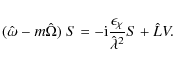
The linear equations for small perturbations in differentially rotating fluids with toroidal magnetic fields were given by Kitchatinov & Rüdiger (2008). Here, the nonmagnetic version of the equations is considered. The equations are formulated for normalized parameters (the rules of conversion to physical variables are given below). The equation for the potential W of the toroidal flow reads

$\displaystyle (\hat{\omega}$	-	$\displaystyle m \hat{\Omega} ) \left(\hat{L}W\right)\ = -{\rm i}\frac{\epsilon_... ...ight) - m \frac{\partial^2\left((1-\mu^2)\hat{\Omega}\right)}{\partial\mu^2}\ W$
	+	$\displaystyle \frac{\partial\left((1-\mu^2)\hat{\Omega}\right)}{\partial\mu} \l... ...)\hat{\Omega}\right)}{\partial\mu^2}\ (1-\mu^2)\frac{\partial V}{\partial\mu} ,$	(3)

where $\hat{\omega} = \omega/\Omega_0$ is the normalized eigenvalue, $\hat{\Omega} = \Omega/\Omega_0$ is the normalized rotation rate, $\mu = \cos\theta$ , V is the poloidal flow potential,

$\begin{displaymath}\hat{L} = \frac{\partial}{\partial\mu}\left(1-\mu^2\right) \frac{\partial}{\partial\mu} - \frac{m^2}{1-\mu^2}\ \ \end{displaymath}$

(4)

is the angular part of the Laplacian operator, and

$\begin{displaymath}\hat{\lambda} = \frac{N}{\Omega_0 kr}\ \ \end{displaymath}$

(5)

is the key parameter for the influence of the stratification. The diffusion terms are characterized by the parameters

$\begin{displaymath}\epsilon_\nu = \frac{\nu N^2}{\Omega_0^3 r^2},\ \ \ \ \ \ \ \... ...\ \ \ \ \ \ \epsilon_\chi = \frac{\chi N^2}{\Omega_0^3 r^2}, \end{displaymath}$

(6)

where $\nu$ and $\chi$ are the microscopic viscosity and the thermal conductivity.

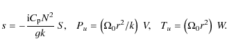
Apart from Eq. (3) for the toroidal flow, the complete system of three equations includes the equation for poloidal flow,

$\displaystyle (\hat{\omega}$	-	$\displaystyle m \hat{\Omega}) \left(\hat{L}V\right)\ = -{\rm i}\frac{\epsilon_\nu}{\hat{\lambda}^2} \left(\hat{L}V\right) - \hat{\lambda}^2 \left(\hat{L}S\right)$
	+	$\displaystyle 2 m\left(\frac{\partial (\mu\hat{\Omega})}{\partial\mu}\ V + (1 -... ...2)\frac{\partial\hat{\Omega}}{\partial\mu}\frac{\partial V}{\partial\mu}\right)$
	-	$\displaystyle 2\mu\hat{\Omega}\left(\hat{L}W\right) - 2 (1-\mu^2)\frac{\partial... ...{\partial W}{\partial\mu} - 2 m^2 \frac{\partial\hat{\Omega}}{\partial\mu}\ W ,$	(7)

and the equation for the normalized entropy S,

$\begin{displaymath}(\hat{\omega} - m \hat{\Omega})\ S = -{\rm i} \frac{\epsilon_\chi}{\hat{\lambda}^2} S + \hat{L}V . \end{displaymath}$

(8)

Equations (3), (7) and (8) form an eigenvalue problem which we solved numerically.

The reason why only latitudinal rotation inhomogeneity is present in the equation system is that radial scale of disturbances is assumed to be short. As a consequence of this assumption, all radial derivatives are absorbed by the disturbances. Contributions of radial derivatives of $\Omega$ such as $\frac{\partial\Omega}{\partial r}\frac{\partial V}{\partial\mu}$ always have a counterpart such as $k V\frac{\partial\Omega}{\partial\mu}$ in the same equation, and the former is always negligible compared to the latter. We note that the radial wave number k is included in the normalization of V (cf. Eq. (8) of Kitchatinov & Rüdiger 2008). Relative magnitude of the omitted terms with radial derivatives of $\Omega$ is the ratio of the radial wave length $\lambda$ of the disturbances to the tachocline thickness w. We shall see that the ratio for most rapidly growing disturbances is lower than one, $\lambda/w \simeq 0.2$ , though not very low.

The values of $\epsilon_\chi = 10^{-4}$ and $\epsilon_\nu = 2\times 10^{-10}$ of the diffusion parameters defined in Eq. (6) are characteristic of the upper radiative core of the Sun and were used. However, close reproduction of some of the results by computations for an ideal fluid with $\epsilon_\chi = \epsilon_\nu = 0$ indicated that the small diffusivities were not significant.

The disturbances in physical units follow from their normalized values by

$\begin{displaymath}s = -\frac{{\rm i} C_{\rm p} N^2}{gk}\ S,\ \ \ P_u = \left(\... ...0 r^2/ k\right)\ V,\ \ \ T_u = \left(\Omega_0 r^2\right)\ W. \end{displaymath}$

(9)

The velocity field can be restored from the potentials of poloidal (P_u) and toroidal (T_u) flows,

$\displaystyle \vec{u}$	=	$\displaystyle \frac{\vec{e}_r}{r^2} \hat{L}P_u - \frac{\vec{e}_\theta}{r} \left... ...ial T_u}{\partial\phi} + \frac{\partial^2 P_u}{\partial r\partial\theta}\right)$
		$\displaystyle +\ \frac{\vec{e}_\phi}{r}\left(\frac{\partial T_u}{\partial\theta} - \frac{1}{\sin\theta}\frac{\partial^2 P_u}{\partial r\partial\phi}\right)$	(10)

(Chandrasekhar 1961), where $\vec{e}_r$ , $\vec{e}_\theta$ , and $\vec{e}_\phi$ are unit vectors in the radial, meridional, and longitudinal directions.

Without rotation ( $\Omega\rightarrow 0$ ) and for small diffusion the Eqs. (3), (7), and (8) reproduce the spectrum

$\begin{displaymath}\omega^2 = \frac{l(l+1) N^2}{r^2k^2},\ \ \ l = 1,2,... \end{displaymath}$

(11)

of g-modes. The limit of very large $\hat\lambda$ -parameter of Eq. (5), which leads to the following 2D approximation, is more relevant to the stability problem.

2.2 2D approximation

The ratio of $N^2/\Omega^2$ in stars can be so high ( $\sim$ 10⁵ in the upper radiative core of the Sun) that $\hat{\lambda}^2$ (5) can also be high in spite of short-wave approximation in radius, $kr \gg 1$ . In the limit of large $\hat{\lambda}^2$ , the above equation system reduces to its 2D approximation. For the leading order of this parameter, Eq. (7) gives S = 0. It then follows from Eq. (8) that V = 0 and that Eq. (3) reduces to the standard equation of 2D theory of Watson (1981),

$\begin{displaymath}\left(\hat{\omega} - m\hat{\Omega}\right)\left(\hat{L}W\right... ...al^2\left((1-\mu^2)\hat{\Omega}\right)} {\partial\mu^2}\ W , \end{displaymath}$

(12)

describing toroidal flows on spherical surfaces.

The 2D approximation is justified for stable oscillations with not too short radial scales so that $\hat\lambda$ remains high. Its validity for stability problem is less certain because the radial scales of most rapidly growing modes are not known in advance and the value of kr for those modes is normally so high that $\hat{\lambda}\lower.4ex\hbox{$\;\buildrel <\over{\scriptstyle\sim}\;$ }1$ (Kitchatinov & Rüdiger 2008).

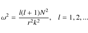
For rigid rotation, Eq. (12) provides the eigenvalue spectrum

$\begin{displaymath}\omega = m\Omega \left( 1 - \frac{2}{l(l+1)}\right),\ \ \ l = 1,2,... \end{displaymath}$

(13)

of the r-modes (Papaloizou & Pringle 1978). Instabilities can emerge with nonuniform rotation. The necessary condition for instability is that the second derivative, ${\rm d}^2((1-\mu^2)\hat{\Omega})/{\rm d}\mu^2$ , changes its sign (Watson 1981). For the angular velocity profile

$\begin{displaymath}\hat{\Omega} = 1 - a\mu^{2n} , \end{displaymath}$

(14)

the condition demands that

$\begin{displaymath}a > \frac{1}{4n+1} \cdot \end{displaymath}$

(15)

It should be a > 0.2 for n=1. For n=2, i.e., the $\cos^4\theta$ -profile in Eq. (14), the amplitude a of the differential rotation at the onset of instability may reduce considerably, i.e., a > 1/9. This is why the $\cos^4\theta$ -term is retained in the differential rotation profile of Eq. (1).

The profile given in Eq. (1) for the Sun is, of course, an approximation. Higher order terms in $\cos^2\theta$ may also be present. The reduction of the instability threshold because of the higher order terms is, however, less significant and they are relevant only to the near-polar regions. Here, the results are presented for the rotation law of Eq. (1).

2.3 Symmetry types

The eigenmodes provided by both the 2D approximation of Eq. (12) and the full 3D equation system of Sect. 2.1 possess definite equatorial symmetries. We use the notation Sm for the modes with symmetric relative to the equator potential W of toroidal flow and the notation Am for antisymmetric W (m is the azimuthal wave number). The symmetry convention is the same as used before (Charbonneau et al. 1999a; Kitchatinov & Rüdiger 2008). We note that the eigenmodes combine W of definite symmetry with S and V of opposite symmetry, i.e., S and Vare symmetric for Am modes and antisymmetric for Sm. The velocity field for Am modes has antisymmetric $u_\theta$ and symmetric u_rand $u_\phi$ about the equatorial plane, and the converse for Sm modes.

Watson (1981) proved that only nonaxisymmetric modes with m=1 and m=2 can be unstable in the 2D approximation. Our 3D computations reach the same conclusion.

3 Results

Figure 1 shows the critical shear amplitudes a as functions of $\hat\lambda$ for f=0. This is the case considered by Watson, and his results are reproduced for the limit of high $\hat\lambda$ . We note, however, that the most easily excited modes have $\hat{\lambda} < 1$ .

$\begin{figure} \par\includegraphics[width=7.8cm]{11842_f1.eps} \end{figure}$	Figure 1: Neutral stability lines for f=0 in rotation law (1). The instability region is above the lines. Only A1 and S2 modes are unstable. The lines approach the marginal a-values of Watson theory for large $\hat\lambda$ . Note that the most unstable modes have $\hat{\lambda} < 1$ .
Open with DEXTER

Even for high $N/\Omega$ , the small radial displacements are significant for the instability. The reason is that the most unstable modes have short radial scales. It can be seen from Eq. (10) that the assumption of zero radial velocity would exclude the entire class of poloidal disturbances. The ratio of horizontal ( $u_{\rm h}$ ) to radial velocities in a cell of poloidal flow of different radial ( $\ell$ ) and horizontal (H) scales can be estimated as $u_{\rm h}/u_r \sim H/\ell$ . Horizontal velocity of poloidal flow can thus remain important in spite of small u_r, if the radial scale is much shorter than the horizontal one. The poloidal (interchange-type) disturbances are so significant for the instability that the critical latitudinal shear for onset of the instability reduces from a=0.28 (value of Watson) to a=0.21. However, this lower value still ensures that the tachocline is stable.

$\begin{figure} \par\includegraphics[width=8.5cm]{11842_f2.eps} \end{figure}$	Figure 2: The same as in Fig. 1 but for f=0.5. The critical shear for onset of the instability is reduced, the newly appeared unstable modes S1 and A2 are excited most easily.
Open with DEXTER

We find that the instability disappears when the stratification approaches adiabaticity ( $N\rightarrow 0$ ). The instability of differential rotation thus does not exist in convection zones.

$\begin{figure} \par\includegraphics[width=9cm]{11842_f3.eps} \end{figure}$	Figure 3: Isolines for the normalized growth rates $\sigma = \Im (\omega )/\Omega _0$ of most rapidly growing modes. Dominating symmetry types are indicated. Dashed lines indicate the watershed between different symmetry types.
Open with DEXTER

Estimations of Sect. 2.2 suggest that finite f in the rotation law of Eq. (1) makes a destabilizing effect. The expectation is confirmed by the results of Fig. 2. The threshold value of a for the onset of the instability is lower than for f=0. New unstable modes appear and the S1 mode is now preferred.

We find that the instability is rather sensitive to the details of the rotation law. The growth rates of the unstable modes depend on a and f as shown in Fig. 3. The length scale $\hat\lambda$ was varied to determine the maximum growth rates shown in the plot. The dashed line separates the regions of different symmetry types. Surprisingly, even the symmetries of the most rapidly growing modes depend on the shape of the rotation law. The shape of the rotation law is the result of the interaction of the turbulence and the basic rotation in the solar/stellar convection zone.

3.1 Angular momentum transport

$\begin{figure} \par\includegraphics[width=9cm]{11842_f4.eps} \end{figure}$	Figure 4: Meridional flux of angular momentum for slightly supercritical ( $\sigma = 0.001$ ) S1-mode for f=0.2 with normalized velocities.
Open with DEXTER

The depth dependence of the solar rotation law known from helioseismology can be interpreted in light of the presented results. The rotation law in the bulk of the almost adiabatically stratified convection zone is stable. In the region of penetrative convection near the base of convection zone, the stratification changes to subadiabaticity and the instability can exist. If it exists, then it reacts back on the differential rotation to cause it to become more of a stable profile with f=0. Our linear computations cannot describe this nonlinear process but they can identify the sense of angular momentum transport. Figure 4 shows that the instability indeed tends to reduce the differential rotation. The plot shows the angular momentum flux $\langle u_\theta u_\phi \rangle$ after longitude-averaging as a function of the latitude. The correlation is negative (positive) for the northern (southern) hemisphere. The angular momentum is thus transported from the equator to the poles. The plot was constructed for slightly supercritical S1 mode, which should be active if the differential rotation is reduced to the marginally stable value (Fig. 3).

3.2 The flow pattern

$\begin{figure} \par\includegraphics[width=9cm]{11842_f5.eps} \end{figure}$	Figure 5: Streamlines of toroidal flow for the same mode as in Fig. 4. Full and dotted lines show opposite senses of circulation.
Open with DEXTER

The streamlines of the toroidal flow for the same S1 mode are shown in Fig. 5. Close to the equator the flow represents transequatorial vortices. The flow pattern drifts in longitude against the direction of rotation in the corotating frame with rates shown in Fig. 6. If the deep-seated vortices were observable (e.g., due to disturbance of the large-scale magnetic field), the observer would see the frequencies

$\begin{displaymath}\nu = m\left(\nu_\odot - \nu_{\rm E}\right) + \nu_\odot\ \hat{\nu} , \end{displaymath}$

(16)

where $\nu_\odot = 450$ nHz is the equatorial rotation frequency of the base of the convection zone, $\nu_{\rm E} = 31.7$ nHz is the orbital rotation frequency of the Earth, and $\hat{\nu}$ is the normalized drift rate shown in Fig. 6. The equation indicates the range of frequencies from about 330 to 350 nHz for the range of drift rates in Fig. 6. The frequencies correspond to periods from about 120 to 160 days for the method of analysis of synoptic maps of solar magnetic fields by Knaack et al. (2005). Two of the periods which Knaack et al. interpret as signatures of r-modes are within this range.

$\begin{figure} \par\includegraphics[width=9cm]{11842_f6.eps} \end{figure}$	Figure 6: Normalized drift rates $\Re (\omega )/\Omega _0 -1$ in corotating frame for slightly supercritical ( $\sigma = 0.001$ ) S1-modes as a function of f-parameter of rotation law in Eq. (1).
Open with DEXTER

4 Discussion

Rotation laws in stably stratified stellar interiors with sufficiently steep latitudinal gradients are hydrodynamically unstable against nonaxisymmetric disturbances or - identically - the r-modes are excited by large enough differential rotation. Since their drift rate is retrograde with an amplitude of about 10% of the rotation rate, they should be observable.

They are only excited, however, in subadiabatically stratified radiative zones and convective overshoot regions. Hence, their existence directly indicates the extended regions of latitudinal shear in the deep stellar interior beneath the proper convection zone. If this region - like the solar tachocline - is thin, then the amplitude of the r-mode oscillation should be much lower than in stars wit extended tachoclines. New calculations that account for radial profiles of the angular velocity are necessary to develop this new r-mode seismology. In the present paper, theradial shear of rotation was not included, which can be justified only if the angular velocity varies with radius on a scale larger than the radial wavelength of unstable excitations. The wavelength can be estimated for the solar tachocline as $\lambda \simeq 10\hat{\lambda}$ Mm (Kitchatinov & Rüdiger 2008). The most easily excited disturbances in Figs. 1 and 2 have the wavelengths $\lambda\simeq 6$ Mm that are shorter than the tachocline width $w\simeq 30$ Mm (Charbonneau et al. 1999b) but not much shorter.

The critical latitudinal shear for the excitation of the modes is not very small. The simplest theory without radial perturbations and with a simplified parabolic rotation law yields a critical latitudinal shear of 28%. We have shown with an improved mathematical analysis that the true value is lower. It is reduced to 21% for the same rotation law but with a 3D theory. The critical shear value is lower still if the rotation law contains a higher order term of $\cos^4\theta$ . Nevertheless, the critical shear rate remains higher than (say) 10%. A rotation law with a slightly smaller latitudinal shear (driven by the turbulence in the convection zone) could stably exist in the stellar interior without any decay. We know, however, that the solar core rotates almost rigidly. This can only be true if the slender solar tachocline is caused by another effect, e.g., by the Maxwell stress of large-scale magnetic fields. They may be of fossil origin since their amplitudes need not exceed (say) 1 Gauss (cf. Rüdiger & Kitchatinov 2007).

If this magnetic concept for the solar tachocline is true and if the tachocline is indeed stable then the very slow decay of the observed lithium abundance is also understandable. The slight increase in the lithium diffusion by one or two orders of magnitude compared to the microscopic diffusivity can be easily explained by slow horizontal motions of order cm/s (see Rüdiger & Pipin 2001) or by radial plumes penetrating from the convection zone (Blöcker et al. 1998).

Acknowledgements

This work was supported by the Deutsche Forschungsgemeinschaft and by the Russian Foundation for Basic Research (project 09-02-91338).

References

Basu, S., & Antia, H. M. 1997, MNRAS, 287, 189 [NASA ADS]
Blöcker, T., Holweger, H., Freytag, B., et al. 1998, Space Sci. Rev., 85, 105 [NASA ADS] [CrossRef] (In the text)
Cally, P. S. 2001, Sol. Phys., 199, 231 [NASA ADS] [CrossRef] (In the text)
Chandrasekhar, S. 1961, Hydrodynamic and Hydromagnetic Stability (Oxford: Clarendon Press), 622 (In the text)
Charbonneau, P., Dikpati, M., & Gilman, P. A. 1999a, ApJ, 526, 523 [NASA ADS] [CrossRef] (In the text)
Charbonneau, P., Christensen-Dalsgaard, J., Henning, R., et al. 1999b, ApJ, 527, 445 [NASA ADS] [CrossRef] (In the text)
Christensen-Dalsgaard, J., Gough, D. O., & Thompson, M. J. 1991, ApJ, 378, 413 [NASA ADS] [CrossRef]
Dziembowski, W., & Kosovichev, A. G. 1987, Acta Astron., 37, 341 [NASA ADS] (In the text)
Garaud, P. 2001, MNRAS, 324, 68 [NASA ADS] [CrossRef] (In the text)
Gilman, P. A. 2005, Astron. Nachr., 326, 208 [NASA ADS] [CrossRef] (In the text)
Howard, R., Adkins, J. M., Boyden, J. E., et al. 1983, Sol. Phys., 83, 321 [NASA ADS] [CrossRef] (In the text)
Kitchatinov, L. L., & Rüdiger, G. 2008, A&A, 478, 1 [NASA ADS] [CrossRef] [EDP Sciences] (In the text)
Knaack, R., Stenflo, J. O., & Berdyugina, S. V. 2005, A&A, 438, 1067 [NASA ADS] [CrossRef] [EDP Sciences] (In the text)
Papaloizou, J., & Pringle, J. E. 1978, MNRAS, 182, 423 [NASA ADS] (In the text)
Rüdiger, G., & Kitchatinov, L. L. 2007, New J. Phys., 9, 302 [CrossRef] (In the text)
Rüdiger, G., & Pipin, V. V. 2001, A&A, 375, 149 [NASA ADS] [CrossRef] [EDP Sciences] (In the text)
Watson, M. 1981, Geophys. Astrophys. Fluid Dyn., 16, 285 [NASA ADS] [CrossRef] (In the text)
Watts, A. L., Andersson, N., Beyer, H., & Schutz, B. F. 2003, MNRAS, 342, 1156 [NASA ADS] [CrossRef] (In the text)

All Figures

$\begin{figure} \par\includegraphics[width=7.8cm]{11842_f1.eps} \end{figure}$	Figure 1: Neutral stability lines for f=0 in rotation law (1). The instability region is above the lines. Only A1 and S2 modes are unstable. The lines approach the marginal a-values of Watson theory for large $\hat\lambda$ . Note that the most unstable modes have $\hat{\lambda} < 1$ .
Open with DEXTER
In the text

$\begin{figure} \par\includegraphics[width=8.5cm]{11842_f2.eps} \end{figure}$	Figure 2: The same as in Fig. 1 but for f=0.5. The critical shear for onset of the instability is reduced, the newly appeared unstable modes S1 and A2 are excited most easily.
Open with DEXTER
In the text

$\begin{figure} \par\includegraphics[width=9cm]{11842_f3.eps} \end{figure}$	Figure 3: Isolines for the normalized growth rates $\sigma = \Im (\omega )/\Omega _0$ of most rapidly growing modes. Dominating symmetry types are indicated. Dashed lines indicate the watershed between different symmetry types.
Open with DEXTER
In the text

$\begin{figure} \par\includegraphics[width=9cm]{11842_f4.eps} \end{figure}$	Figure 4: Meridional flux of angular momentum for slightly supercritical ( $\sigma = 0.001$ ) S1-mode for f=0.2 with normalized velocities.
Open with DEXTER
In the text

$\begin{figure} \par\includegraphics[width=9cm]{11842_f5.eps} \end{figure}$	Figure 5: Streamlines of toroidal flow for the same mode as in Fig. 4. Full and dotted lines show opposite senses of circulation.
Open with DEXTER
In the text

$\begin{figure} \par\includegraphics[width=9cm]{11842_f6.eps} \end{figure}$	Figure 6: Normalized drift rates $\Re (\omega )/\Omega _0 -1$ in corotating frame for slightly supercritical ( $\sigma = 0.001$ ) S1-modes as a function of f-parameter of rotation law in Eq. (1).
Open with DEXTER
In the text

Current usage metrics show cumulative count of Article Views (full-text article views including HTML views, PDF and ePub downloads, according to the available data) and Abstracts Views on Vision4Press platform.

Data correspond to usage on the plateform after 2015. The current usage metrics is available 48-96 hours after online publication and is updated daily on week days.

Initial download of the metrics may take a while.