| Issue |
A&A
Volume 504, Number 1, September II 2009
|
|
|---|---|---|
| Page(s) | 1 - 13 | |
| Section | Cosmology (including clusters of galaxies) | |
| DOI | https://doi.org/10.1051/0004-6361/20079006 | |
| Published online | 02 July 2009 | |
Weak lensing density profiles and mass reconstructions
of the galaxy clusters Abell 1351 and Abell 1995![[*]](/icons/foot_motif.png)
K. Holhjem1,2 - M. Schirmer1,3 - H. Dahle2
1 - Argelander-Institut für Astronomie (AIfA), Universität Bonn,
Auf dem Hügel 71, 53121 Bonn, Germany
2 - Institute of Theoretical Astrophysics, University of Oslo, PO Box
1029 Blindern, 0315 Oslo, Norway
3 - Isaac Newton Group of Telescopes, Calle Alvarez Abreu 70,
38700 Santa Cruz de La Palma, Spain
Received 6 November 2007 / Accepted 11 June 2009
Abstract
Aims. The aim of the present work is to study the overall mass distribution of the galaxy clusters Abell 1351 and Abell 1995 using weak gravitational lensing. These clusters have a very different mass structure and dynamical state and are the two extremes from a larger sample of 38 X-ray luminous clusters of similar size and redshift.
Methods. We measure the shear values of faint background galaxies and correct for PSF anisotropies using the KSB+ method. Two-dimensional mass maps of the clusters are created using a finite-field mass reconstruction algorithm, and verified with aperture mass statistics. The masses inferred from the reconstructions are compared to those obtained from fitting spherically symmetric SIS- and NFW-models to the tangential shear profiles. We discuss the NFW concentration parameters in detail.
Results. From the mass reconstructions we infer
![]() -masses of
-masses of
![]() and
and
![]() for Abell 1351 and Abell 1995, respectively. About
for Abell 1351 and Abell 1995, respectively. About
![]() northeast of the main mass peak of Abell 1351, we detect a significant secondary peak both in the mass reconstruction and from aperture mass statistics. This feature is also traced by cluster members selected by means of their V-I colour, and is therefore likely a real substructure of Abell 1351. From our fits to the tangential shear we infer masses of the order of
northeast of the main mass peak of Abell 1351, we detect a significant secondary peak both in the mass reconstruction and from aperture mass statistics. This feature is also traced by cluster members selected by means of their V-I colour, and is therefore likely a real substructure of Abell 1351. From our fits to the tangential shear we infer masses of the order of
![]() (Abell 1351) and
(Abell 1351) and
![]() (Abell 1995). The concentration parameters remain poorly constrained by our weak lensing analysis.
(Abell 1995). The concentration parameters remain poorly constrained by our weak lensing analysis.
Key words: gravitational lensing - cosmology: dark matter - galaxies: clusters: individual: Abell 1351, Abell 1995
1 Introduction
Comprising the most massive gravitationally bound structures in the Universe, galaxy clusters are essential in providing a deeper understanding of the properties of dark matter. The recent papers covering 1E 0657-558 (the bullet cluster) by Clowe et al. (2006a) and Abell 520 by Mahdavi et al. (2007) demonstrate the importance of gravitational lensing for understanding the matter content of our Universe. Lensing studies of galaxy clusters provide a powerful way to identify high density peaks in the Universe, independent of their baryonic content (Schirmer et al. 2007; Miyazaki et al. 2007; Clowe et al. 2006b; Maturi et al. 2007; Dahle et al. 2003; Gavazzi & Soucail 2007; Schneider 1996; Wittman et al. 2006).
Neither the nature nor the dynamical state of the gravitating matter affect the mass estimates obtained through gravitational lensing. These mass measurements are only changed by gravitation and the geometrical configuration between observer, lens, and source. Although this makes lensing a unique tool, such measurements can be biased by e.g. different mass concentrations along the line-of-sight.
In this paper we analyse two clusters of galaxies at intermediate
redshift (z=0.32), Abell 1351 and Abell 1995. These clusters
are selected from a lensing study of 38 highly X-ray luminous galaxy
clusters (Dahle et al. 2002). They were chosen for further investigation
because they represent the two extremes in this cluster sample,
regarding mass distribution and dynamical state. Re-observing the
clusters with the wide-field camera CFH12K at the Canada-France-Hawaii
telescope (CFHT) provided a larger field of view
(
![]() )
than employed by Dahle et al. (2002)
(
)
than employed by Dahle et al. (2002)
(
![]() ). This allows us to map the
clusters to larger radii than previously possible.
). This allows us to map the
clusters to larger radii than previously possible.
The KSB+ method (Luppino & Kaiser 1997; Kaiser et al. 1995; Hoekstra et al. 1998) is used to recover the shear values of faint background galaxies in the images. Using a finite-field reconstruction technique (Seitz & Schneider 2001), we derive two-dimensional mass maps, visualising the surface mass distributions of Abell 1351 and Abell 1995. We also apply aperture mass statistics (Schirmer et al. 2007; Schneider 1996) to our data, comparing the results to confirm mass peak detections. Finally, by fitting predicted shear values from theoretical models to the shapes of the lensed galaxies we estimate the cluster masses. We assume the clusters to be spherically symmetric and to have density profiles following either a singular isothermal sphere (SIS) or a Navarro, Frenk, & White 1997, 1995; NFW model.
Data processing and analysis are carried out using mainly the IMCAT software package![]() , Kaiser's July
2005 version for Macintosh. IMCAT is a tool specially designed
for weak lensing purposes, and is optimised for shape measurements of
faint galaxies. It processes both FITS files and object
catalogues.
, Kaiser's July
2005 version for Macintosh. IMCAT is a tool specially designed
for weak lensing purposes, and is optimised for shape measurements of
faint galaxies. It processes both FITS files and object
catalogues.
The outline of this paper is as follows. In Sect. 2 we summarise the observations and software used for our study, in addition to the data reduction. In Sect. 3 we describe the shear reconstruction, focusing on shape estimates and point spread function (PSF) corrections. In Sect. 4 we present the clusters' surface mass density maps and attempt to verify the detected mass peaks using V-I colours and aperture mass statistics. By comparing the measured shear profiles to theoretical expectations, we model the lensing data in Sect. 5. Finally we present and discuss our results in Sect. 6, and our conclusions in Sect. 7.
Throughout this paper we assume a ![]() CDM cosmology,
with
CDM cosmology,
with
![]() ,
,
![]() ,
and
h70=H0/(70 km s-1 Mpc-1). Errors are given on
the
,
and
h70=H0/(70 km s-1 Mpc-1). Errors are given on
the ![]() level.
level.
2 Observations and data reduction
2.1 Data acquisition
The galaxy clusters Abell 1351 and Abell 1995 are centred at the
positions
![]() and
and
![]() ,
respectively. They were observed with the CFHT on the 4
nights of 7-11 May, 2000, using the wide-field CCD mosaic camera
CFH12K. A total exposure time of 5400 s was obtained for both clusters
in I band. However, due to seeing >
,
respectively. They were observed with the CFHT on the 4
nights of 7-11 May, 2000, using the wide-field CCD mosaic camera
CFH12K. A total exposure time of 5400 s was obtained for both clusters
in I band. However, due to seeing >
![]() ,
we
rejected 3 exposures from the Abell 1351 data set, resulting in 3600 s
for this cluster. This corresponds to a
,
we
rejected 3 exposures from the Abell 1351 data set, resulting in 3600 s
for this cluster. This corresponds to a ![]() limiting magnitude
of
limiting magnitude
of
![]() for point sources in both pointings. The seeing in
the final coadded images equals
for point sources in both pointings. The seeing in
the final coadded images equals
![]() and
and
![]() for
Abell 1351 and Abell 1995, respectively. The number density of the
lensed background galaxies is 16 arcmin-2 for both clusters,
and the ellipticity dispersion (after PSF correction) for each
component is
for
Abell 1351 and Abell 1995, respectively. The number density of the
lensed background galaxies is 16 arcmin-2 for both clusters,
and the ellipticity dispersion (after PSF correction) for each
component is
![]() and
and
![]() for Abell 1351 and
Abell 1995, respectively. The larger dispersion for Abell 1995 is
explained by the
for Abell 1351 and
Abell 1995, respectively. The larger dispersion for Abell 1995 is
explained by the ![]() larger image seeing, which enlarges the PSF
correction factors and their uncertainties.
larger image seeing, which enlarges the PSF
correction factors and their uncertainties.
The CFH12K mosaic camera covers a field of
![]() pixels in total, representing an area
of
pixels in total, representing an area
of
![]() on the sky. The pixel scale is
on the sky. The pixel scale is
![]() when mounted at the CFHT prime focus.
when mounted at the CFHT prime focus.
In addition we made use of the V-band data obtained by
Dahle et al. (2002) to verify neighbouring peaks present in our
two-dimensional mass maps described in Sect. 4. These data
were obtained at the 2.24 m University of Hawaii telescope using the
UH8K mosaic camera, covering an area of
![]() pixels (rebinned
pixels (rebinned ![]() )
mapping
)
mapping
![]() of the sky. Each image has a
total exposure time of 12 600 s, resulting in a depth comparable to
our I-band data, with
of the sky. Each image has a
total exposure time of 12 600 s, resulting in a depth comparable to
our I-band data, with ![]() limiting magnitudes of
limiting magnitudes of
![]() and
and
![]() for Abell 1351 and Abell 1995,
respectively. Further details about the reduction process and
coaddition of the V-band data can be found in Dahle et al. (2002).
for Abell 1351 and Abell 1995,
respectively. Further details about the reduction process and
coaddition of the V-band data can be found in Dahle et al. (2002).
As Abell 1351 and Abell 1995 are both located at redshift z=0.32,
they have a similar correspondence between physical and angular scale,
given as
![]() .
.
2.2 Image processing
2.2.1 Pre-processing
To remove the bias level in each frame we used the mean value of the overscan region from the corresponding chip. The flatfielding was carried out using a master night time flat, made from averaging 56 night time exposures; most of them so-called ``blank'' fields and all well displaced from each other. The fringing that occurs in I-band exposures is also captured in this type of flat, and upon dividing the object exposures by it the fringes were cleanly removed. To estimate the background level in the exposures, we used the heights of the minima of the sky level present to create a model for each individual frame. After subtraction the median sky level was set to zero.
As fringing is an additive effect and not a multiplicative one,
ideally the fringes should be subtracted. Since we had no twilight
flats available, standard defringing could not be performed. The
photometric error introduced by division is negligible, as the
amplitude of the fringes compared to the sky background after
flatfielding was of the order of ![]() .
However, since fringing acts
mostly on small angular scales, its treatment will affect the shapes
of the small and faint background galaxies used for weak lensing. To
investigate this we obtained a set of 10 archival images of the Deep3
field (Hildebrandt et al. 2006), taken with the Wide Field Imager at the 2.2 m
MPG/ESO telescope through their I-band filter. As the Deep3 field
does not contain any massive clusters it is very well suited for this
test. Two different coadded images were created. In the first case the
data were flatfielded using twilight flats, after which a fringing
model was created from the flatfielded data and subtracted. The second
coadded image was processed in the same way as our CFHT data, i.e. the
data were flatfielded and fringe-corrected by division of a night-time
flat. We then measured the shapes of a common set of
.
However, since fringing acts
mostly on small angular scales, its treatment will affect the shapes
of the small and faint background galaxies used for weak lensing. To
investigate this we obtained a set of 10 archival images of the Deep3
field (Hildebrandt et al. 2006), taken with the Wide Field Imager at the 2.2 m
MPG/ESO telescope through their I-band filter. As the Deep3 field
does not contain any massive clusters it is very well suited for this
test. Two different coadded images were created. In the first case the
data were flatfielded using twilight flats, after which a fringing
model was created from the flatfielded data and subtracted. The second
coadded image was processed in the same way as our CFHT data, i.e. the
data were flatfielded and fringe-corrected by division of a night-time
flat. We then measured the shapes of a common set of ![]() 12 000 galaxies in both images (see Sect. 3) and created two mass
reconstructions, using the same technique and smoothing scale as for
Abell 1351 and Abell 1995 (see Sect. 4). We found that the
rms of the difference of the two mass maps is a factor of 2.5 smaller
than the noise of the individual mass maps, mainly caused by the
intrinsic ellipticities of background galaxies. The effect in our
CFH12K data is much smaller, as the CFH12K I-band filter has a
blue cut-on at around 730 nm and a red cut-off at 950 nm. The ESO
I-band filter on the other hand opens at 800 nm and has no
cut-off on the red side. Hence the fringing amplitude in the
comparison data set from ESO is up to 5 times higher than that from
CFHT. We conclude that our analysis of Abell 1351 and Abell 1995 is
not affected by our fringe correction.
12 000 galaxies in both images (see Sect. 3) and created two mass
reconstructions, using the same technique and smoothing scale as for
Abell 1351 and Abell 1995 (see Sect. 4). We found that the
rms of the difference of the two mass maps is a factor of 2.5 smaller
than the noise of the individual mass maps, mainly caused by the
intrinsic ellipticities of background galaxies. The effect in our
CFH12K data is much smaller, as the CFH12K I-band filter has a
blue cut-on at around 730 nm and a red cut-off at 950 nm. The ESO
I-band filter on the other hand opens at 800 nm and has no
cut-off on the red side. Hence the fringing amplitude in the
comparison data set from ESO is up to 5 times higher than that from
CFHT. We conclude that our analysis of Abell 1351 and Abell 1995 is
not affected by our fringe correction.
![\begin{figure}
\par\includegraphics[width=17cm]{79006fg1.ps}
\end{figure}](/articles/aa/full_html/2009/34/aa9006-07/img44.png) |
Figure 1: Example of size-magnitude ( left) and weighted ellipticity parameter diagram ( right) for an arbitrary exposure. The moderately bright, non-saturated stars were chosen from within the squares and utilised in the astrometric solution, the right plot containing only the stars chosen from the left plot. The stars utilised in the PSF corrections (Sect. 3.1) were selected the same way. |
| Open with DEXTER | |
2.2.2 Masking
The CFH12K mosaic contains some bad pixels and columns, in particular
two of the CCDs suffer from this. By using Nick Kaiser's ready made
CFH12K masks![]() as global
masks, all bad areas were ensured to be ignored. An additional patch
of 219 bad columns in CCD00 was also added to the global masks. We did
not make further individual masks for each exposure, as most spurious
detections were filtered out during the astrometric calibration.
Suspicious objects in the final catalogue were in addition rejected by
visual examination.
as global
masks, all bad areas were ensured to be ignored. An additional patch
of 219 bad columns in CCD00 was also added to the global masks. We did
not make further individual masks for each exposure, as most spurious
detections were filtered out during the astrometric calibration.
Suspicious objects in the final catalogue were in addition rejected by
visual examination.
2.2.3 Astrometric calibration
Wide-field data typically do not have a simple relation between the sky coordinates and those of the detector. A mapping from pixel coordinates onto a planar projection of the sky needs therefore be performed. We solved for this through a series of steps.
First, all objects in each exposure were detected and aperture
photometry carried out. By plotting rg (![]() half-light radius)
vs. instrumental magnitude of the objects in each exposure, we
extracted the moderately bright, non-saturated stars suitable for
deriving an astrometric solution. Their weighted ellipticity
parameters (defined by Kaiser et al. 1995), e1,2, were in addition
plotted and eyeballed, and the main clustering of objects were
selected to ensure a catalogue containing purely stars (see
Fig. 1 for an example). IMCAT only offers squared
regions for extracting objects from a two-dimensional parameter
space. Although a circle would be a more natural choice for the right
panel in Fig. 1, the difference is considered negligible.
half-light radius)
vs. instrumental magnitude of the objects in each exposure, we
extracted the moderately bright, non-saturated stars suitable for
deriving an astrometric solution. Their weighted ellipticity
parameters (defined by Kaiser et al. 1995), e1,2, were in addition
plotted and eyeballed, and the main clustering of objects were
selected to ensure a catalogue containing purely stars (see
Fig. 1 for an example). IMCAT only offers squared
regions for extracting objects from a two-dimensional parameter
space. Although a circle would be a more natural choice for the right
panel in Fig. 1, the difference is considered negligible.
Left with star catalogues we then computed the transformation
parameters needed using information from the USNO-B1.0 catalogue
(Monet et al. 2003). However, as many of the USNO-B1.0 stars were saturated
in our images, we extended our reference catalogue by detecting more
sources in FITS files derived from the Digitized Sky
Survey![]() . We
matched the target catalogues to the reference catalogue, solving for
a set of low-order spatial polynomials mapping the images onto each
other, by repeatedly refining the least squares minimisations using
outlier rejection.
. We
matched the target catalogues to the reference catalogue, solving for
a set of low-order spatial polynomials mapping the images onto each
other, by repeatedly refining the least squares minimisations using
outlier rejection.
2.2.4 Final master image and object catalogue
Gain and quantum efficiency variations between chips and differential
extinction between exposures were solved for by least squares
minimisations. The extinction corrections between the exposures were
very small, typically ![]() 0.01 mag, whereas the zero-point
offsets between the chips were
0.01 mag, whereas the zero-point
offsets between the chips were ![]() 0.1 mag. As an accurate
absolute photometric calibration was not necessary for the present
work, we adopted standard Landolt magnitude zeropoints.
0.1 mag. As an accurate
absolute photometric calibration was not necessary for the present
work, we adopted standard Landolt magnitude zeropoints.
The coaddition was done after magnitude corrections were applied to the data. In addition cosmic rays were masked out, before the median image was computed and the background flattened. A master object catalogue was created, where each object's WCS coordinates were calculated from the astrometric solution, and their ellipticity parameters computed (see Sect. 3). Finally we masked out false detections by overplotting the objects onto the image, hence ensuring a final object catalogue free from spurious detections.
3 Shear measurements
Identifying weak lensing effects requires measuring the ellipticities of a large number of faint background galaxies. The main source of noise in weak lensing analysis is the intrinsic ellipticities of these galaxies. To distinguish between distorted images resulting from a weak lens and the usual distribution of shapes existing in an unlensed galaxy population, the ellipticities must be examined for a systematic change. In particular, a tangential alignment of the galaxy shapes around the cluster centre would confirm the existence of a weak lens.
An additional source of error comes from the faint background galaxies being smeared by the PSF, caused by atmospheric turbulence and optical aberrations. The weak shear signal is hence diluted because this smearing will cause the galaxy images to appear more circular than before the smearing. In addition, PSF anisotropies distort the images, causing the galaxies to appear more elliptical, hence introducing false shear signals. It is crucial that these PSF effects are corrected for.
3.1 PSF corrections
Following the KSB+ method developed by Kaiser et al. (1995), Luppino & Kaiser (1997), and Hoekstra et al. (1998), we present a short summary of our implementation below. KSB+ inverts the effects of PSF smearing and anisotropy on objects in an image, presenting a method to recover the true shear.
![\begin{figure}
\par\includegraphics[width=16.5cm]{79006fg2.ps}
\end{figure}](/articles/aa/full_html/2009/34/aa9006-07/img45.png) |
Figure 2:
Ellipticities of the stars in the field of Abell 1351 ( top)
and Abell 1995 ( bottom) before and after corrections for PSF
anisotropies. The stars initially had systematic ellipticities up
to |
| Open with DEXTER | |
Ignoring the effects of photon noise, it is possible to
express the observed ellipticity of a galaxy as
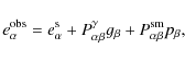
where the first term represents the intrinsic ellipticity of the galaxy, the second term the shift in ellipticity caused by gravitational shear, and the third term the smearing of the galaxy image from the anisotropic PSF see Luppino & Kaiser 1997, with additional corrections from Hoekstra et al. 1998 for a thorough deduction of this equation. Present in Eq. (1) are the pre-seeing shear polarisability tensor,
Because stars are foreground objects (![]() )
and intrinsically
circular (
)
and intrinsically
circular (
![]() ), applying Eq. (1) to stellar
objects provides a measure of the total PSF anisotropy,
), applying Eq. (1) to stellar
objects provides a measure of the total PSF anisotropy, ![]() .
This was calculated from bright stars selected from the
final object catalogue (Sect. 2.2.4). The PSF corrections were
then calculated for all individual objects and corrections applied
respectively.
.
This was calculated from bright stars selected from the
final object catalogue (Sect. 2.2.4). The PSF corrections were
then calculated for all individual objects and corrections applied
respectively.
The ellipticities of the stars were fitted to a sixth-order Taylor series expansion. When comparing mass and B-mode maps (Sect. 4) for fits of different orders, there was little change with the order of fit. Over the whole field, 410 and 530 stars were used in the fitting process for Abell 1351 and Abell 1995 respectively. Figure 2 shows the ellipticities of the stars before and after PSF corrections.
The pre-seeing shear polarisability tensor,
![]() ,
is defined in KSB+ to be
,
is defined in KSB+ to be
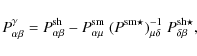
where the asterisk denotes
![\begin{displaymath}
g_\beta = (P^\gamma)^{-1}_{\alpha\beta}
\left[e_\alpha^{\rm obs} - P^{\rm sm}_{\alpha\beta}p_\beta\right]
.
\end{displaymath}](/articles/aa/full_html/2009/34/aa9006-07/img58.png)
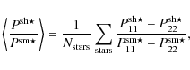
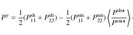
Following the approach by Wold et al. (2002), we assume the PSF is close to circular after the correction, and the polarisabilities can be approximated by
 |
(4) |
where using the median value rather than the mean minimises the effect of outliers. Hence Eq. (2) turns into
As
Table 1: Results from fitting theoretical density profiles to the measured shear values, where each subheadline indicates the cluster centre around which the fitting was done.
Hoekstra et al. (1998) showed that estimating the PSF dilution for each
individual galaxy introduces additional noise. We therefore followed
their approach by determining ![]() as a function of magnitude
and galaxy size. We determined the median
as a function of magnitude
and galaxy size. We determined the median ![]() within 15 bins in
an rg-magnitude diagram, where the central 4 bins contain
within 15 bins in
an rg-magnitude diagram, where the central 4 bins contain
![]() 4000 galaxies/bin and the outer ones
4000 galaxies/bin and the outer ones ![]() 200 galaxies/bin. We
then computed one correction factor for each bin using
Eq. (5), and applied this to all galaxies within the
corresponding bin.
200 galaxies/bin. We
then computed one correction factor for each bin using
Eq. (5), and applied this to all galaxies within the
corresponding bin.
The faintest and smallest galaxies are more affected by seeing than
the larger galaxies, giving them a poorer shape determination and a
high correction factor. Such galaxies are therefore of less
importance. To account for this, a normalised weight,

was calculated for each bin i and assigned to the corresponding galaxies. Here,
4 Mass reconstruction
We selected background galaxies with
6<S/N<100 for the
creation of our mass maps. These maps were constructed from the
galaxies' shapes using the finite-field inversion method presented by
Seitz & Schneider 2001; SS01. This method
calculates a smoothed shear field on a grid using a modified Gaussian
filter. The algorithm then iteratively computes a quantity
![]() which is determined up to
an additive constant due to the mass sheet degeneracy. We could break
this degeneracy by assuming that the average convergence vanishes
along the border of the wide field of view. The width of the Gaussian
term in the filter was set to
which is determined up to
an additive constant due to the mass sheet degeneracy. We could break
this degeneracy by assuming that the average convergence vanishes
along the border of the wide field of view. The width of the Gaussian
term in the filter was set to
![]() ,
resulting in an effective
smoothing length of about
,
resulting in an effective
smoothing length of about
![]() .
.
In order to evaluate the noise of the mass maps, we computed 2000 mass maps for each cluster based on randomised galaxy orientations, keeping their positions fixed. As the cluster lens signal increases the ellipticities of galaxies, this would lead to an overestimation of the noise at the cluster position. We roughly corrected for this effect by subtracting the expected SIS tangential shear signal, determined from the clusters' known velocity dispersions (see Table 1). Since the singularity of the SIS can lead to overly large corrections close to the cluster centre, we limited the maximum correction factor allowed to 0.5 in each ellipticity component. This affected less than 5 galaxies in both fields. The true mass maps were then divided by the noise maps obtained from the randomised mass maps to create the S/N-maps seen in Fig. 3.
Abell 1351 and Abell 1995 are detected with a S/N of 5.3 and 5.2,
respectively. Upon integrating the ![]() maps within
maps within
![]() (
(
![]() )
for Abell 1351 (Abell 1995), we find total masses of
)
for Abell 1351 (Abell 1995), we find total masses of
![]() and
and
![]() for the clusters, respectively. The r200 radii have been taken
from what we consider to be the best NFW fits to the data (see
Table 1 and Sect. 5.2), while the errors were
determined from integrating the same areas in the 2000 noise maps.
for the clusters, respectively. The r200 radii have been taken
from what we consider to be the best NFW fits to the data (see
Table 1 and Sect. 5.2), while the errors were
determined from integrating the same areas in the 2000 noise maps.
The B-modes in both cluster fields are shown in Fig. 3,
computed by repeating the ![]() reconstruction with all galaxies
rotated
reconstruction with all galaxies
rotated
![]() (Crittenden et al. 2002). Provided that the lensing data are
free from systematics and that the noise (intrinsic ellipticities) is
Gaussian, these B-mode maps should be consistent with Gaussian
noise. Given the effective filter scale of
(Crittenden et al. 2002). Provided that the lensing data are
free from systematics and that the noise (intrinsic ellipticities) is
Gaussian, these B-mode maps should be consistent with Gaussian
noise. Given the effective filter scale of
![]() ,
about 380 independent peaks can be placed in the CFH12K field. Thus one would
expect 1.1 noise peaks above
,
about 380 independent peaks can be placed in the CFH12K field. Thus one would
expect 1.1 noise peaks above ![]() in the field. A more
realistic estimate comes from the 2000 randomisations as these are
based on the real ellipticity and spatial distribution. We expect 1.4 (1.6) such peaks for Abell 1351 (Abell 1995). In the real
B-mode maps we find 3 peaks for each of the clusters. This is
insignificant, as in our randomisations at least 3 such peaks appear
per field in
in the field. A more
realistic estimate comes from the 2000 randomisations as these are
based on the real ellipticity and spatial distribution. We expect 1.4 (1.6) such peaks for Abell 1351 (Abell 1995). In the real
B-mode maps we find 3 peaks for each of the clusters. This is
insignificant, as in our randomisations at least 3 such peaks appear
per field in ![]() of the cases. In case of Abell 1995 the highest
B-mode peak has a significance of
of the cases. In case of Abell 1995 the highest
B-mode peak has a significance of ![]() .
Its B-modes appear
generally somewhat larger than for Abell 1351, which has no B-mode
peaks higher than
.
Its B-modes appear
generally somewhat larger than for Abell 1351, which has no B-mode
peaks higher than ![]() .
.
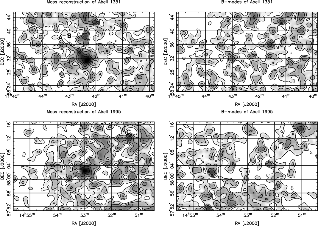 |
Figure 3:
The projected surface mass densities and B-modes for both clusters
in the full CFH12K field, using a finite-field mass
reconstruction. The maps show the S/N of the clusters, with
contours starting at |
| Open with DEXTER | |
4.1 Mass and galaxy density distributions
In order to compare the surface density maps with the distribution of
cluster galaxies, we extracted the red sequence (see
e.g. Gladders & Yee 2000) and investigated the distribution of the selected
galaxies. To match the I-band and the V-band images, we
resampled both data sets to the same pixel scale, resulting in a
common area of
![]() on the sky. The
V-band image seeing is around
on the sky. The
V-band image seeing is around
![]() ,
and thus consistently
better than in the I-band. The V-band data were
therefore convolved to match the seeing in the I-band data,
,
and thus consistently
better than in the I-band. The V-band data were
therefore convolved to match the seeing in the I-band data,
![]() for Abell 1351 and
for Abell 1351 and
![]() for Abell 1995. Aperture
photometry was carried out using SExtractor (Bertin & Arnouts 1996) in
double-image mode. The deep I-band images served as the
detection image, providing us with a target list with defined
coordinates. At these positions we integrated the flux in a
for Abell 1995. Aperture
photometry was carried out using SExtractor (Bertin & Arnouts 1996) in
double-image mode. The deep I-band images served as the
detection image, providing us with a target list with defined
coordinates. At these positions we integrated the flux in a
![]() wide aperture in each of the V- and I-band
images. Plotting the galaxies in a colour-magnitude diagram will then
in principle provide enough information to separate the red early-type
cluster members from the other galaxies.
wide aperture in each of the V- and I-band
images. Plotting the galaxies in a colour-magnitude diagram will then
in principle provide enough information to separate the red early-type
cluster members from the other galaxies.
Each cluster's red sequence did not clearly stand out from the
V-I vs. I diagram when all objects were plotted.
However, selecting only galaxies within a radius of
![]() of the
brightest cluster galaxy (BCG) for the colour-magnitude diagram (see
Fig. 4) enabled us to detect a red sequence at
1.4<V-I<1.9 for both clusters. The selection criteria
indicated by the box in each plot were then applied to the entire
object catalogue. The number density of the galaxies selected was then
calculated as a function of position and overplotted onto the
central
of the
brightest cluster galaxy (BCG) for the colour-magnitude diagram (see
Fig. 4) enabled us to detect a red sequence at
1.4<V-I<1.9 for both clusters. The selection criteria
indicated by the box in each plot were then applied to the entire
object catalogue. The number density of the galaxies selected was then
calculated as a function of position and overplotted onto the
central
![]() of the mass maps (see Fig. 5).
of the mass maps (see Fig. 5).
The number density maps were normalised by the fluctuation measured in
the field outside the clusters. The centres of Abell 1351 and
Abell 1995 are then detected with
![]() and
and ![]() significance, respectively. The positional offsets between mass
centres, BCGs, and centres of galaxy density distributions are in
the range of
significance, respectively. The positional offsets between mass
centres, BCGs, and centres of galaxy density distributions are in
the range of
![]() for both clusters, and are
due to noise in the mass maps. Changing the width of the Gaussian
kernel in the finite-field reconstruction algorithm shows that the
peak centres can drift by up to
for both clusters, and are
due to noise in the mass maps. Changing the width of the Gaussian
kernel in the finite-field reconstruction algorithm shows that the
peak centres can drift by up to
![]() from the mean
position. These offsets are consistent with other results in the
literature, such as Clowe et al. (2006a), who observed offsets of the order
of
from the mean
position. These offsets are consistent with other results in the
literature, such as Clowe et al. (2006a), who observed offsets of the order
of
![]() between the lensing peaks (of higher S/N than ours) and
the optical centres of the bullet cluster. Positional offsets
of
between the lensing peaks (of higher S/N than ours) and
the optical centres of the bullet cluster. Positional offsets
of
![]() are common in the sample of 70 shear-selected clusters
by Schirmer et al. (2007).
are common in the sample of 70 shear-selected clusters
by Schirmer et al. (2007).
The cluster galaxy distribution resembles well the mass distribution in the central part of Abell 1351. It extends significantly towards the northeast, a feature also seen in the mass map where we find a local maximum which we refer to as peak A (see Sect. 4.2). The galaxy distribution of Abell 1995 appears elliptical and elongated in the northeast-southwest direction. This property is not reflected in the mass map where the peak is of rather circular appearance.
To check the integrity of our mass reconstructions further, we applied the
peak finder (S-statistics) developed by Schirmer et al. (2007). This method
detects areas of enhanced tangential shear using the aperture mass statistics
(Schneider 1996). Since it uses a filter function that mimics the tangential
shear profile of galaxy clusters it is well suited for detecting mass
concentrations. With this method we recover Abell 1351 at the ![]() level in a
level in a
![]() wide filter, and Abell 1995 with
wide filter, and Abell 1995 with ![]() for a
for a
![]() filter. The filter shape parameter (Schirmer et al. 2007) was chosen as
filter. The filter shape parameter (Schirmer et al. 2007) was chosen as
![]() in both cases. We find that the S-statistics is elongated in
the same way as the mass reconstruction for Abell 1351, extending towards peak
A. We evaluate the significance of this possible substructure in
the following.
in both cases. We find that the S-statistics is elongated in
the same way as the mass reconstruction for Abell 1351, extending towards peak
A. We evaluate the significance of this possible substructure in
the following.
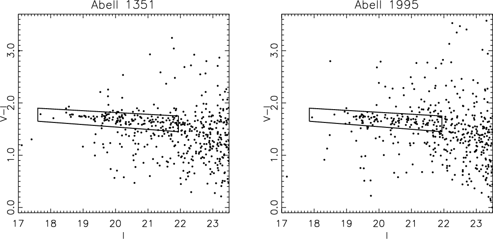 |
Figure 4:
Colour-magnitude diagrams for Abell 1351 ( left) and
Abell 1995 ( right), where only galaxies within
|
| Open with DEXTER | |
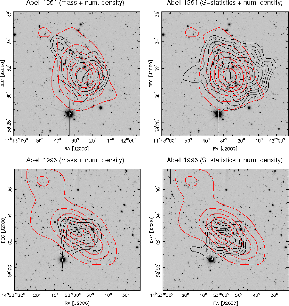 |
Figure 5:
The black contours show the mass reconstruction ( left) and
S-statistics ( right) for Abell 1351 ( top) and Abell 1995
( bottom). The contours start at the |
| Open with DEXTER | |
4.2 Lower mass peaks in the fields
In the mass reconstructions two neighbouring peaks A and B are
detected around Abell 1351, and another one (peak C) in the field of
Abell 1995. Their S/N-ratios are 4.2, 3.8, and 3.8,
respectively. We used the 2000 noise randomisations for each field to
find that the probability of a noise peak higher than ![]() (
(![]() )
in the field of Abell 1351 is
)
in the field of Abell 1351 is ![]() (
(![]() ),
respectively. The corresponding probability for peak C in the
Abell 1995 data is
),
respectively. The corresponding probability for peak C in the
Abell 1995 data is ![]() .
These are somewhat higher
than what would be expected from purely Gaussian noise.
.
These are somewhat higher
than what would be expected from purely Gaussian noise.
Hence the only significant substructure detected in the mass
reconstructions is peak A near Abell 1351. Looking at the contours in
the upper right panel of Fig. 5, one can see that the
S-statistics trace this structure as well at the
![]() -level. We note that we recovered this substructure
over a broad range of filter scales in the S-statistics and hence
think that it is a real feature in the mass distribution of
Abell 1351.
-level. We note that we recovered this substructure
over a broad range of filter scales in the S-statistics and hence
think that it is a real feature in the mass distribution of
Abell 1351.
Out of the broad range (
![]() )
of filters probed
with the S-statistics, peak B is detected only once with
)
of filters probed
with the S-statistics, peak B is detected only once with
![]() in the
in the
![]() wide filter for
wide filter for
![]() .
It has
the typical characteristics of the dark peaks found by Schirmer et al. (2007),
i.e. it is not associated with any overdensity of galaxies. It is
therefore most likely a noise peak.
.
It has
the typical characteristics of the dark peaks found by Schirmer et al. (2007),
i.e. it is not associated with any overdensity of galaxies. It is
therefore most likely a noise peak.
In the Abell 1995 field we could not detect any other peaks
using the S-statistics. Since the B-modes for those data show
a maximum of ![]() near peak C (at
near peak C (at ![]() ), we
consider it to be a noise peak. As it also lies outside the area
covered by the V-band, we could not check for overdensities of
red galaxies at this position.
), we
consider it to be a noise peak. As it also lies outside the area
covered by the V-band, we could not check for overdensities of
red galaxies at this position.
5 Modelling the lensing data
The mass of a galaxy cluster can be estimated by comparing observed
distortions in the background galaxies to those predicted by
theoretical density profiles. Using ![]() -minimisations of SIS and
NFW models we first determined the best fit parameters and then
calculated the cluster masses.
-minimisations of SIS and
NFW models we first determined the best fit parameters and then
calculated the cluster masses.
The theoretical profiles are both spherically symmetric. We therefore
averaged the tangential reduced shear,
![]() (for
(for
![]() ,
where
,
where
![]() is the Einstein radius), in 17 radial bins
around the cluster centre. The bins are logarithmically spaced,
covering the entire field of view, and starting at
is the Einstein radius), in 17 radial bins
around the cluster centre. The bins are logarithmically spaced,
covering the entire field of view, and starting at
![]() to avoid the large contamination from cluster
galaxies close to the centre of the field (see also
Sect. 5.1). To determine the cluster centre, we
tested three different positions. First we adopted the peak location
in the mass reconstructions generated (Sect. 4). These
coincide with the centres of the S-statistics. Second the BCG
served as cluster centre, and third we tried the centre of the galaxy
density of each cluster. As the last coincide with the BCG for
Abell 1995, only two positions were tested for this cluster.
We also considered strong lensing features, but found that they
do not offer further insight in this respect (see
Sect. 6.3.1 for details). We calculated
to avoid the large contamination from cluster
galaxies close to the centre of the field (see also
Sect. 5.1). To determine the cluster centre, we
tested three different positions. First we adopted the peak location
in the mass reconstructions generated (Sect. 4). These
coincide with the centres of the S-statistics. Second the BCG
served as cluster centre, and third we tried the centre of the galaxy
density of each cluster. As the last coincide with the BCG for
Abell 1995, only two positions were tested for this cluster.
We also considered strong lensing features, but found that they
do not offer further insight in this respect (see
Sect. 6.3.1 for details). We calculated
![]() for each radial bin i and compared them
to the theoretical values at the average radius of each bin,
for each radial bin i and compared them
to the theoretical values at the average radius of each bin,
![]() .
.
When calculating the mass of a cluster, the relative distance of the
background galaxies and the lensing cluster is required. As we have no
specific information about the redshifts of the background galaxies,
the distances had to be estimated statistically. By using the
photometric redshift distribution of corresponding faint galaxies from
the Hubble Deep Field North (Fernández-Soto et al. 1999), we estimated the
average
![]() ,
where
,
where
![]() is the angular diameter distance between the lens and the source
and Ds between the observer and the source. The empirical relation
is the angular diameter distance between the lens and the source
and Ds between the observer and the source. The empirical relation
| (7) |
is derived for a
5.1 Cluster contamination and magnification depletion
At small projected radii from the cluster centre our faint galaxy
sample will contain cluster galaxies in addition to background
galaxies. We could not discriminate faint cluster members from
lensed field galaxies using V-I colours, hence the sample of
presumed lensed background galaxies remained contaminated, leading to
a systematic bias of the shear measurements towards lower values.
In order to quantify this contamination, we determined the overdensity
of galaxies in the background catalogue at the cluster position
compared to the mean density in the field (an example is shown in
Fig. 6 for Abell 1351). A contamination rate of ![]() was found for both cluster centres, vanishing for radii larger
than about
was found for both cluster centres, vanishing for radii larger
than about
![]() .
.
The cluster galaxy contamination is in fact even higher than stated
above, as magnification depletion leads to a reduced number density of
lensed galaxies in the I-band near the cluster centre. We
found, however, that this effect can be neglected in our case. From
the smoothed convergence (see Sect. 4) and reduced shear
fields we estimated the magnification using
![]() .
We found very similar magnifications for
both clusters, being 1.65 at the centre and becoming
indistinguishable from the noise (
.
We found very similar magnifications for
both clusters, being 1.65 at the centre and becoming
indistinguishable from the noise (
![]() )
for radii
larger than
)
for radii
larger than ![]()
![]() .
The depletion of the number density of
lensed galaxies is
.
The depletion of the number density of
lensed galaxies is
![]() ,
with s=0.15 in red filters
(see e.g. Narayan & Bartelmann 1996). At the cluster centres the number densities
are thus reduced by a factor of
,
with s=0.15 in red filters
(see e.g. Narayan & Bartelmann 1996). At the cluster centres the number densities
are thus reduced by a factor of ![]() ,
and at a radius of
,
and at a radius of
![]() magnification depletion becomes indistinguishable from the
natural fluctuations in the distribution of field
galaxies. Magnification depletion hence only affects the innermost
magnification depletion becomes indistinguishable from the
natural fluctuations in the distribution of field
galaxies. Magnification depletion hence only affects the innermost
![]()
![]() (
(
![]() )
of the clusters and can be
neglected since we compare the tangential shear profiles to models
only for radii larger than
)
of the clusters and can be
neglected since we compare the tangential shear profiles to models
only for radii larger than
![]() (see
Fig. 7).
(see
Fig. 7).
In order to correct for the contamination by cluster galaxies, we
modified the theoretical shear values. The reason for adjusting the
theoretical values rather than the measured values is that this method
is considerably easier to implement. The correction factors were
determined in radial bins of logarithmic spacing. One correction value
was then calculated for each of the 17 bins in which
![]() had been measured. By assuming the
edges of the field to be approximately free from cluster galaxies, the
outermost correction factor could be set to 1 to mimic
contamination-free boundaries of the field. Finally the best fit was
found using
had been measured. By assuming the
edges of the field to be approximately free from cluster galaxies, the
outermost correction factor could be set to 1 to mimic
contamination-free boundaries of the field. Finally the best fit was
found using ![]() -minimisations.
-minimisations.
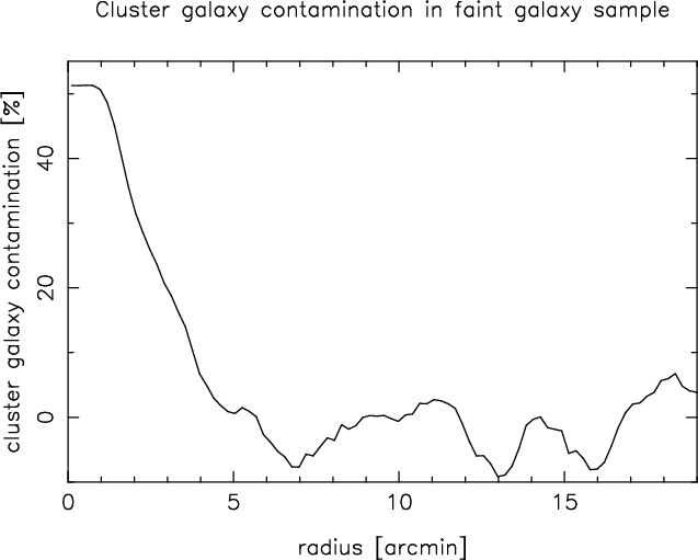 |
Figure 6:
Percentage of cluster galaxies in the faint galaxy
catalogue of Abell 1351 (that of Abell 1995 is very
similar). Because the projected density of cluster
galaxies is assumed to equal zero at the edge of the field, the
cluster galaxy contamination was set to zero here by subtracting
the median value outside the central area of the image (the
large field of view makes this a well-working approximation). Our
fitting procedure starts at
|
| Open with DEXTER | |
5.2 Fitting the SIS and the NFW profiles
Once the cluster centre is determined, the only free parameter of the
SIS profile is the velocity dispersion, ![]() .
The best fit of
the SIS profile is determined by
.
The best fit of
the SIS profile is determined by ![]() -minimisation for a range of
-minimisation for a range of
![]() values, the results being shown in Table 1. The
mass estimate,
values, the results being shown in Table 1. The
mass estimate,
![]() ,
for this profile is calculated at r200 (the radius inside which the mean mass density of the
cluster equals
,
for this profile is calculated at r200 (the radius inside which the mean mass density of the
cluster equals
![]() )
found in the NFW fitting with two
free parameters utilising the same cluster centre.
)
found in the NFW fitting with two
free parameters utilising the same cluster centre.
The NFW profile is derived from fitting the density profiles of
numerically simulated cold dark matter halos. It appears to give a
very good description of the radial mass distribution inside the
virial radius of a galaxy cluster. For a thorough introduction to the
gravitational lensing properties of the NFW mass density profile
we refer the reader to Wright & Brainerd (2000). The theoretical
![]() and
and ![]() can be calculated analytically for the NFW density
profile (Bartelmann & Schneider 2001). We derived the best fit parameters for different
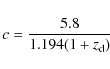
values of the concentration parameter, c, ranging from 0.1 to 24.9 in steps of 0.1.
can be calculated analytically for the NFW density
profile (Bartelmann & Schneider 2001). We derived the best fit parameters for different
values of the concentration parameter, c, ranging from 0.1 to 24.9 in steps of 0.1.
With the cluster centre fixed, the NFW profile has two free
parameters, r200 and c. We fitted our shear measurements to
this profile twice; first by keeping c fixed and varying only r200 to find our best fit, and second by varying both
parameters. The best fit parameters were determined by minimising ![]() in both cases. Based on N-body simulations of dark matter
halos, Bullock et al. (2001) derived relations for the mean value of c as a
function of redshift and mass for different cosmologies. For a halo of
mass
in both cases. Based on N-body simulations of dark matter
halos, Bullock et al. (2001) derived relations for the mean value of c as a
function of redshift and mass for different cosmologies. For a halo of
mass
![]() ,
the relation yields
,
the relation yields
(where
As an example we display the reduced tangential shear as a function of
radius using the SS01 ![]() maps as cluster centre, see the left
diagrams of Fig. 7. The measured values of
maps as cluster centre, see the left
diagrams of Fig. 7. The measured values of
![]() are given together with the best fit models
of the SIS and NFW profiles. Judging from the diagrams alone, the NFW
profile letting both c and r200 vary seems to represent the
best fit to the clusters. However, the
are given together with the best fit models
of the SIS and NFW profiles. Judging from the diagrams alone, the NFW
profile letting both c and r200 vary seems to represent the
best fit to the clusters. However, the
![]() values given
for each model in Table 1 show that the differences
between the models are not statistically significant. The differences
emerging from different cluster centres seem to have a higher
impact. The right diagrams of Fig. 7 show the B-modes
of both clusters, i.e. the cross-component of
values given
for each model in Table 1 show that the differences
between the models are not statistically significant. The differences
emerging from different cluster centres seem to have a higher
impact. The right diagrams of Fig. 7 show the B-modes
of both clusters, i.e. the cross-component of
![]() as a function of radius. Both measurements are consistent with zero.
as a function of radius. Both measurements are consistent with zero.
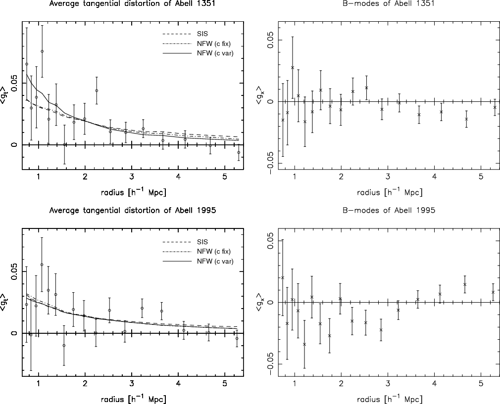 |
Figure 7:
Left: Reduced tangential shear as a function of
radius for Abell 1351 ( top) and Abell 1995 ( bottom) using the SS01
|
| Open with DEXTER | |
6 Discussion
X-ray studies show Abell 1351 to be a galaxy cluster exhibiting
significant dynamical activity and undergoing a major merger event
(Allen et al. 2003), which indicates a cluster still in its formation
phase. Analyses assuming a relaxed cluster will hence naturally differ
from weak lensing analyses, where no assumption is made about the
dynamical state of the cluster. One example is the virial analysis by
Irgens et al. (2002), where an unusually high velocity dispersion of
![]() km s-1 was obtained for
Abell 1351, based on radial velocity measurements of 17 cluster
galaxies. Such a high velocity dispersion is not uncommon in merging
systems. If for example two smaller clusters with low velocity
dispersions fall towards each other along the line of sight with
a velocity comparable to or higher than their
km s-1 was obtained for
Abell 1351, based on radial velocity measurements of 17 cluster
galaxies. Such a high velocity dispersion is not uncommon in merging
systems. If for example two smaller clusters with low velocity
dispersions fall towards each other along the line of sight with
a velocity comparable to or higher than their ![]() ,
then
a very large total
,
then
a very large total ![]() would be inferred, with a
correspondingly overestimated virial mass. The cluster
CL
0056.03-37.55 is a good example for such a system
(see Schirmer et al. 2003).
would be inferred, with a
correspondingly overestimated virial mass. The cluster
CL
0056.03-37.55 is a good example for such a system
(see Schirmer et al. 2003).
Abell 1995 is, unlike Abell 1351, classified as a relaxed cluster in dynamical equilibrium (Pedersen & Dahle 2007). X-ray studies and virial analyses of this cluster are hence also more compatible with lensing studies (Irgens et al. 2002; Patel et al. 2000). The projected two-dimensional distribution of cluster galaxies in Abell 1995 is clearly elliptical (see Fig. 5), whereas the central lensing mass distribution is circular.
6.1 The mass estimates
The mass distributions of Abell 1351 and Abell 1995 were estimated assuming that the clusters follow spherically symmetric SIS or NFW profiles. Although an elliptical mass profile might yield more accurate cluster mass estimations, Dietrich et al. (2005) showed that the results from fitting a singular isothermal ellipse model depend strongly on the initial values chosen for the minimisation routines. We therefore decided not to fit this profile to our clusters.
Heymans et al. (2006) demonstrated in the shear testing programme that the
KSB+ PSF correction tends to systematically underestimate the shear
values ![]()
![]() .
To measure how much this affects our
data, we calculated an upper limit for our mass estimates by increasing
the ellipticities with
.
To measure how much this affects our
data, we calculated an upper limit for our mass estimates by increasing
the ellipticities with ![]() and repeating the fitting process. We
found that the underestimation of shear leads to an underestimation of
the total cluster mass with a maximum of
and repeating the fitting process. We
found that the underestimation of shear leads to an underestimation of
the total cluster mass with a maximum of ![]() ,
which is within the
initial error bars. The concentration parameters did not change
significantly by this boosting of ellipticities. Since we do not know
by exactly how much our shear values are underestimated this was
merely an attempt to quantify this effect on our data, and is not
taken into account in the results presented in this paper.
,
which is within the
initial error bars. The concentration parameters did not change
significantly by this boosting of ellipticities. Since we do not know
by exactly how much our shear values are underestimated this was
merely an attempt to quantify this effect on our data, and is not
taken into account in the results presented in this paper.
Dahle et al. (2002) obtained weak lensing estimates of the cluster velocity
dispersion of several clusters using an SIS model and assuming an
Einstein-de Sitter universe. Their results were
![]() for Abell 1351
and
for Abell 1351
and
![]() for Abell 1995, and
do not agree with our results. However, there are several important
differences in methodology between Dahle et al. (2002) and our work. As
mentioned above, the assumed cosmological model is different. Also,
the first paper approximated
for Abell 1995, and
do not agree with our results. However, there are several important
differences in methodology between Dahle et al. (2002) and our work. As
mentioned above, the assumed cosmological model is different. Also,
the first paper approximated
![]() ,
whereas
we use
,
whereas
we use
![]() in our fits and
mass reconstructions. Finally, the shear estimator of Kaiser (2000)
used by Dahle et al. (2002) is shown by Heymans et al. (2006) to have a non-linear
response to shear. A re-analysis of the Dahle et al. (2002) data, taking all
these effects into account, yielded new values of
in our fits and
mass reconstructions. Finally, the shear estimator of Kaiser (2000)
used by Dahle et al. (2002) is shown by Heymans et al. (2006) to have a non-linear
response to shear. A re-analysis of the Dahle et al. (2002) data, taking all
these effects into account, yielded new values of
![]() and
and
![]() for Abell 1351 and
Abell 1995, respectively. Hence there still remains a systematic
discrepancy between the results for Abell 1351, while the measurements
for Abell 1995 agree within error bars.
for Abell 1351 and
Abell 1995, respectively. Hence there still remains a systematic
discrepancy between the results for Abell 1351, while the measurements
for Abell 1995 agree within error bars.
A remaining difference between our work and Dahle et al. (2002) is the
maximum radius,
![]() ,
to which the shear is measured, given by the field of
view of the detector. Changing
,
to which the shear is measured, given by the field of
view of the detector. Changing
![]() in our Abell 1351 data to
in our Abell 1351 data to
![]() as this is the value used by Dahle et al. 2002
led to
as this is the value used by Dahle et al. 2002
led to
![]() ,
consistent with
the re-analysed Dahle et al. (2002) values within error bars.
,
consistent with
the re-analysed Dahle et al. (2002) values within error bars.
Allen et al. (2003) used the Dahle et al. (2002) observations to obtain a weak
lensing mass estimate applying the NFW model to a ![]() CDM
cosmology. Their results gave
CDM
cosmology. Their results gave
![]() for
Abell 1351 and
for
Abell 1351 and
![]() for
Abell 1995. These values are high compared to the results of this
study. Allen et al. (2003) used a fixed concentration parameter in the
fitting process, c=5. Applying this value to our data yielded
minimal changes in M200. The discrepancies hence originate from
Allen et al. (2003) utilising
for
Abell 1995. These values are high compared to the results of this
study. Allen et al. (2003) used a fixed concentration parameter in the
fitting process, c=5. Applying this value to our data yielded
minimal changes in M200. The discrepancies hence originate from
Allen et al. (2003) utilising
![]() and
and
![]() (priv. comm.) for Abell 1351 and Abell 1995, respectively, as these
values are larger than our best fit r200 values.
(priv. comm.) for Abell 1351 and Abell 1995, respectively, as these
values are larger than our best fit r200 values.
6.2 The concentration parameter
The mass density of a cluster with a low concentration parameter
decreases slower when going to larger radii than for a cluster with a
high c value (Wright & Brainerd 2000). Although unconstrained upwards, we find a
lower limit of ![]() for Abell 1351. As is also seen from the
radial dependence of the shear in Fig. 7 (top left),
the mass distribution of Abell 1351 concentrates around the cluster
centre, indicating that its concentration parameter is significantly
higher than that of Abell 1995. The values found for c of Abell 1995
(see Table 1) suggest that its mass is spread more evenly
to larger radii, which is also seen in Fig. 7 (bottom
left).
for Abell 1351. As is also seen from the
radial dependence of the shear in Fig. 7 (top left),
the mass distribution of Abell 1351 concentrates around the cluster
centre, indicating that its concentration parameter is significantly
higher than that of Abell 1995. The values found for c of Abell 1995
(see Table 1) suggest that its mass is spread more evenly
to larger radii, which is also seen in Fig. 7 (bottom
left).
Table 2: Results from varying the inner radius from where the shear values of Abell 1351 are measured.
From their aperture mass calculations Dahle et al. (2002) found that most of
the mass of Abell 1995 is contained within
![]() (
(![]()
![]() ). The mass of
Abell 1351 shows the opposite behaviour, increasing evenly with radius,
even at large radii. These results are contrary to our conclusions.
As measurements at large radii are certain to include additional
information not recognised close to the cluster centre, these
discrepancies are likely explained by the difference in
field-size between the two studies. By mapping the mass distribution
towards a radius more than twice the size as that of Dahle et al. (2002),
our results are better constrained. Further bias also arises from the
measurements of Dahle et al. (2002) starting from an inner radius of
). The mass of
Abell 1351 shows the opposite behaviour, increasing evenly with radius,
even at large radii. These results are contrary to our conclusions.
As measurements at large radii are certain to include additional
information not recognised close to the cluster centre, these
discrepancies are likely explained by the difference in
field-size between the two studies. By mapping the mass distribution
towards a radius more than twice the size as that of Dahle et al. (2002),
our results are better constrained. Further bias also arises from the
measurements of Dahle et al. (2002) starting from an inner radius of
![]() ,
where we consider the cluster galaxy contamination to be very high, in
addition to not including any correction for this contamination.
,
where we consider the cluster galaxy contamination to be very high, in
addition to not including any correction for this contamination.
Our shear values are measured from a radial cut-off,
![]() ,
to avoid the large cluster galaxy
contamination present at small radii. Because c is estimated from
the scale radius,
,
to avoid the large cluster galaxy
contamination present at small radii. Because c is estimated from
the scale radius,
![]() ,
it is desirable to include
,
it is desirable to include ![]() in
the measurements (
in
the measurements (
![]() )
in order to obtain an
accurate estimate of the concentration parameter. If this is not the
case, c is basically unconstrained.
)
in order to obtain an
accurate estimate of the concentration parameter. If this is not the
case, c is basically unconstrained.
This appears to be the case for Abell 1351, explaining why we were not
able to derive an upper limit for its concentration parameter. Letting
![]() ,
we ensured a cluster galaxy
contamination <25% at this inner radius. However, as the
c parameter appears unconstrained under this condition, we reduced
,
we ensured a cluster galaxy
contamination <25% at this inner radius. However, as the
c parameter appears unconstrained under this condition, we reduced
![]() in an attempt to obtain clearer results. The problem
then arising was the increasing contamination of cluster
galaxies. Looking at Fig. 6 we see that at
in an attempt to obtain clearer results. The problem
then arising was the increasing contamination of cluster
galaxies. Looking at Fig. 6 we see that at
![]() the cluster contamination is
the cluster contamination is ![]() 32%, and at
32%, and at
![]() it equals
it equals ![]() 40%. Though this contamination
is accounted for during the fitting process, the contamination
correction is still vulnerable to fluctuations in the projected galaxy
density caused by foreground and/or background structures.
40%. Though this contamination
is accounted for during the fitting process, the contamination
correction is still vulnerable to fluctuations in the projected galaxy
density caused by foreground and/or background structures.
Table 2 presents the results from letting
![]() for Abell 1351
(with the Kaiser & Squires 1993
for Abell 1351
(with the Kaiser & Squires 1993 ![]() map peak as cluster centre, see
Sect. 6.3). It
is seen that whilst c is decreasing with smaller
map peak as cluster centre, see
Sect. 6.3). It
is seen that whilst c is decreasing with smaller
![]() ,
r200 and M200 remain stable for different
,
r200 and M200 remain stable for different
![]() .
Also worth noticing is that for
.
Also worth noticing is that for
![]() ,
c becomes
constrained. However, as
,
c becomes
constrained. However, as
![]() for the different starting
radii, we cannot obtain further conclusions from these results. As
for the different starting
radii, we cannot obtain further conclusions from these results. As
![]() is even smaller for Abell 1995, we did not repeat this test for
the cluster. Dietrich et al. (2005) experienced similar problems when
attempting to determine the concentration parameter for Abell 222 and
Abell 223, concluding that obtaining a reliable c from weak lensing
data only is difficult, if not impossible.
is even smaller for Abell 1995, we did not repeat this test for
the cluster. Dietrich et al. (2005) experienced similar problems when
attempting to determine the concentration parameter for Abell 222 and
Abell 223, concluding that obtaining a reliable c from weak lensing
data only is difficult, if not impossible.
6.2.1 Best fit concentration parameter
Bullock et al. (2001) presented dark matter halo simulations, attempting to find
a ``best fit concentration parameter'' applicable to all types of
halos. They found that for halos of the same mass, the concentration,
![]() ,
can be given by
,
can be given by
![]() .
This is contrary to
earlier beliefs that
.
This is contrary to
earlier beliefs that
![]() does not vary much with
redshift. Numerically simulated massive clusters typically have
concentration parameters
does not vary much with
redshift. Numerically simulated massive clusters typically have
concentration parameters ![]() 4-5 (Bullock et al. 2001).
This is within the limiting values for both clusters, although looking
at Fig. 7, the outcome from varying c seems to better
follow the shear values of Abell 1351.
4-5 (Bullock et al. 2001).
This is within the limiting values for both clusters, although looking
at Fig. 7, the outcome from varying c seems to better
follow the shear values of Abell 1351.
There exists several examples of high concentration parameters in the
literature. Kneib et al. (2003) found
![]() for the
central mass concentration of the cluster
for the
central mass concentration of the cluster
![]() .
Gavazzi (2005) concluded on
.
Gavazzi (2005) concluded on
![]() for
for
![]() ,
while
Broadhurst et al. (2005) found
,
while
Broadhurst et al. (2005) found
![]() for
Abell 1689. Limousin et al. (2007) presented a thorough discussion of the
different concentration parameters derived for Abell 1689 in the
literature, concluding that a distribution of best fit cparameters is needed for observed lensing clusters in order to provide
a sample large enough to make an adequate comparison with
simulations. A recent study of observed concentration values for
clusters by Comerford & Natarajan (2007) show that the best fit lensing-derived cparameters are systematically higher than concentrations derived via
X-ray measurements, a difference which can be at least partly
explained by effects of triaxiality of cluster halos
(Gavazzi 2005; Corless & King 2007; Clowe et al. 2004; Oguri et al. 2005) or the substructure within the clusters
(King & Corless 2007), although the latter effect may also produce a negative
bias of c values. In addition, baryonic physics can increase the
concentration parameter mildly by up to
for
Abell 1689. Limousin et al. (2007) presented a thorough discussion of the
different concentration parameters derived for Abell 1689 in the
literature, concluding that a distribution of best fit cparameters is needed for observed lensing clusters in order to provide
a sample large enough to make an adequate comparison with
simulations. A recent study of observed concentration values for
clusters by Comerford & Natarajan (2007) show that the best fit lensing-derived cparameters are systematically higher than concentrations derived via
X-ray measurements, a difference which can be at least partly
explained by effects of triaxiality of cluster halos
(Gavazzi 2005; Corless & King 2007; Clowe et al. 2004; Oguri et al. 2005) or the substructure within the clusters
(King & Corless 2007), although the latter effect may also produce a negative
bias of c values. In addition, baryonic physics can increase the
concentration parameter mildly by up to ![]() as compared to
dissipationless dark matter in pure dark matter simulations (see
e.g. Lin et al. 2006).
as compared to
dissipationless dark matter in pure dark matter simulations (see
e.g. Lin et al. 2006).
6.3 Centre position
In addition to the three centre positions tested in Sect. 5,
we computed ![]() maps with the inversion method of
Kaiser & Squires 1993; KS93 and utilised the
peak of this surface mass distribution as a fourth cluster centre. The
KS93 method assumes that
maps with the inversion method of
Kaiser & Squires 1993; KS93 and utilised the
peak of this surface mass distribution as a fourth cluster centre. The
KS93 method assumes that ![]() ,
which is not a good approximation
near the centres of massive systems. Therefore, in comparison with the
other methods, it provided us with a reference point as for how large
variation one can reasonably expect for the various centroiding
methods.
,
which is not a good approximation
near the centres of massive systems. Therefore, in comparison with the
other methods, it provided us with a reference point as for how large
variation one can reasonably expect for the various centroiding
methods.
All centre positions obtained with the four methods lie within
![]() and hence represent the errors expected when using the peak of
a
and hence represent the errors expected when using the peak of
a ![]() map as cluster centre. As can be seen from Table 1,
varying the centre position only slightly can lead to different mass
estimates. Although within error bars, the results from fitting NFW
using a fixed c varies most. The NFW fitting of two parameters is
more stable with a smaller spread in M200. This is also reflected
in
map as cluster centre. As can be seen from Table 1,
varying the centre position only slightly can lead to different mass
estimates. Although within error bars, the results from fitting NFW
using a fixed c varies most. The NFW fitting of two parameters is
more stable with a smaller spread in M200. This is also reflected
in
![]() ,
as a value closer to 1 is a better fit.
,
as a value closer to 1 is a better fit.
Worth noticing is the generally smaller differences between the results of Abell 1995 as compared to those of Abell 1351. The concentration parameter also seems better constrained for Abell 1995, where we could not obtain an upper limit for c only in the case where the BCG was used as the centre reference. On the other hand, an upper limit for c could not be obtained for Abell 1351 for any of the cluster centres chosen. This is consistent with the fact that Abell 1351 is not in dynamical equilibrium, lacking a well-defined cluster centre. The results obtained from fitting spherically symmetric models hence depend on the cluster centre chosen.
6.3.1 Strong lensing features
Strong lensing effects are in general susceptive to substructures in clusters, and might constrain the centre of mass further. For both clusters recent archival WFPC2 HST data exists, taken for an ongoing snapshot survey of X-ray luminous clusters (HST PID 11103, PI: H. Ebeling). The images are taken through the F606W filter totalling 1200 s exposure time each.
Taking into account both the colours and morphologies of galaxies in our V-I data and the morphologies in the HST images, there are at least half a dozen plausible arcs and arclets visible in each of the two clusters. The lensing pattern for Abell 1351 appears to be very complex and does not indicate a single, well-defined centre. This is supported by the presence of several elliptical galaxies which are of similar brightness as the BCG. On the contrary, for Abell 1995 several arc(let)s are well aligned around the BCG (apart from three which are obviously associated with individual cluster galaxies), justifying adopting the BCG as cluster centre for Abell 1995. Applying strong lensing to our data will therefore not offer further constraints on the determination of the centre of mass than we already have.
6.4 The mass reconstructions
In Sect. 4 we presented the weak lensing reconstruction of
the clusters' surface mass density, detecting the clusters on the
![]() level. In case of Abell 1351 a significant neighbouring peak
A was detected, which coincides with the galaxy distribution.
level. In case of Abell 1351 a significant neighbouring peak
A was detected, which coincides with the galaxy distribution.
We note significant differences comparing our mass maps to those of
Dahle et al. (2002), who used the KS93 inversion method. Abell 1995
appears rather circular in both reconstructions, with attached filamentary
structures of low significance seen in the KS93 map. In their re-analysis of
the Abell 901 supercluster field, Heymans et al. (2008) argued that such filamentary
structures could be enhanced by the KS93 method itself. This algorithm
assumes ![]() near the critical cluster cores, which hence overestimates
near the critical cluster cores, which hence overestimates ![]() ,
and the smoothing implemented could then lead to the apparent
merging of neighbouring peaks.
,
and the smoothing implemented could then lead to the apparent
merging of neighbouring peaks.
Our map of Abell 1351 appears roughly circular at the position of the main cluster with a significant extension towards the northeast, whereas it shows an extension to the southwest in the work of Dahle et al. (2002). Both reconstructions have peak B in common. Since it is not associated with any overdensity of galaxies but appears in both reconstructions based on very different data sets, the most likely explanation is a chance alignment of galaxies triggering this detection.
7 Conclusions
Utilising observations from CFH12K we find the masses of Abell 1351
(Abell 1995) to be
![]() (
(
![]() ). These results are
derived from fitting our data to the NFW profile, altering both cand r200, to find the best theoretical fit to our shear
measurements (Fig. 7). Our
). These results are
derived from fitting our data to the NFW profile, altering both cand r200, to find the best theoretical fit to our shear
measurements (Fig. 7). Our ![]() reconstructions
yield mass estimates of
reconstructions
yield mass estimates of
![]() (
(
![]() )
for
Abell 1351 (Abell 1995).
)
for
Abell 1351 (Abell 1995).
Our results illustrate that using solely weak lensing measurements,
with no photometric or spectroscopic information to separate cluster
members from background galaxies, the concentration parameter found
for a galaxy cluster is poorly constrained. Future spectroscopic
redshift measurements and strong lens modelling of the arcs seen
towards the cores of Abell 1351 and Abell 1995 might help improve the
constraints on their concentration parameters. However, the change
in c value resulting from small variations of the centre position of
Abell 1351 indicates that the mass distribution in the core of this
dynamically unrelaxed cluster is too complex to be meaningfully fit by
the NFW mass density profile. M200, on the other hand, varies
only slightly for both clusters when either
![]() is decreased
or the cluster centre varied. Although the KSB+ PSF correction leads
to an underestimation of the cluster masses (with a maximum of
is decreased
or the cluster centre varied. Although the KSB+ PSF correction leads
to an underestimation of the cluster masses (with a maximum of ![]() in our case), increasing the background galaxy ellipticities
correspondingly still yields masses within error bars of our current
estimates. We therefore conclude that the mass estimates presented are
robust.
in our case), increasing the background galaxy ellipticities
correspondingly still yields masses within error bars of our current
estimates. We therefore conclude that the mass estimates presented are
robust.
Acknowledgements
The authors thank the anonymous referee for very helpful critics, and Thomas Erben and Peter Schneider for useful and constructive comments. We also thank Aleksi Halkola for helpful discussion during the NFW analysis. K.H. gratefully acknowledges support from a doctoral fellowship awarded by the Research council of Norway, project number 177254/V30.
References
- Allen, S. W., Schmidt, R. W., Fabian, A. C., & Ebeling, H. 2003, MNRAS, 342, 287 [NASA ADS] [CrossRef] (In the text)
- Bartelmann, M., & Schneider, P. 2001, Phys. Rep., 340, 291 [NASA ADS] [CrossRef] (In the text)
- Bertin, E., & Arnouts, S. 1996, A&AS, 117, 393 [NASA ADS] [CrossRef] [EDP Sciences] (In the text)
- Broadhurst, T., Takada, M., Umetsu, K., et al. 2005, ApJ, 619, L143 [NASA ADS] [CrossRef] (In the text)
- Bullock, J. S., Kolatt, T. S., Sigad, Y., et al. 2001, MNRAS, 321, 559 [NASA ADS] [CrossRef] (In the text)
- Clowe, D., De Lucia, G., & King, L. 2004, MNRAS, 350, 1038 [NASA ADS] [CrossRef]
- Clowe, D., Bradac, M., Gonzalez, A. H., et al. 2006a, ApJ, 648, L109 [NASA ADS] [CrossRef] (In the text)
- Clowe, D., Schneider, P., Aragón-Salamanca, A., et al. 2006b, A&A, 451, 395 [NASA ADS] [CrossRef] [EDP Sciences]
- Comerford, J. M., & Natarajan, P. 2007, MNRAS, 379, 190 [NASA ADS] [CrossRef] (In the text)
- Corless, V. L., & King, L. J. 2007, MNRAS, 380, 149 [NASA ADS] [CrossRef]
- Crittenden, R. G., Natarajan, P., Pen, U.-L., & Theuns, T. 2002, ApJ, 568, 20 [NASA ADS] [CrossRef] (In the text)
- Dahle, H., Kaiser, N., Irgens, R. J., Lilje, P. B., & Maddox, S. J. 2002, ApJS, 139, 313 [NASA ADS] [CrossRef] (In the text)
- Dahle, H., Pedersen, K., Lilje, P. B., Maddox, S. J., & Kaiser, N. 2003, ApJ, 591, 662 [NASA ADS] [CrossRef]
- Dietrich, J. P., Schneider, P., Clowe, D., Romano-Díaz, E., & Kerp, J. 2005, A&A, 440, 453 [NASA ADS] [CrossRef] [EDP Sciences] (In the text)
- Fernández-Soto, A., Lanzetta, K. M., & Yahil, A. 1999, ApJ, 513, 34 [NASA ADS] [CrossRef] (In the text)
- Gavazzi, R. 2005, A&A, 443, 793 [NASA ADS] [CrossRef] [EDP Sciences] (In the text)
- Gavazzi, R., & Soucail, G. 2007, A&A, 462, 459 [NASA ADS] [CrossRef] [EDP Sciences]
- Gladders, M., & Yee, H. 2000, AJ, 120, 2148 [NASA ADS] [CrossRef] (In the text)
- Heymans, C., Van Waerbeke, L., Bacon, D., et al. 2006, MNRAS, 368, 1323 [NASA ADS] [CrossRef] (In the text)
- Heymans, C., Gray, M. E., Peng, C. Y., et al. 2008, MNRAS, 385, 1431 [NASA ADS] [CrossRef] (In the text)
- Hildebrandt, H., Erben, T., Dietrich, J. P., et al. 2006, A&A, 452, 1121 [NASA ADS] [CrossRef] [EDP Sciences] (In the text)
- Hoekstra, H., Franx, M., Kuijken, K., & Squires, G. 1998, ApJ, 504, 636 [NASA ADS] [CrossRef]
- Irgens, R. J., Lilje, P. B., Dahle, H., & Maddox, S. J. 2002, ApJ, 579, 227 [NASA ADS] [CrossRef] (In the text)
- Kaiser, N. 2000, ApJ, 537, 555 [NASA ADS] [CrossRef] (In the text)
- Kaiser, N., & Squires, G. 1993, ApJ, 404, 441 [NASA ADS] [CrossRef] (In the text)
- Kaiser, N., Squires, G., & Broadhurst, T. 1995, ApJ, 449, 460 [NASA ADS] [CrossRef]
- King, L., & Corless, V. 2007, MNRAS, 374, L37 [NASA ADS] (In the text)
- Kneib, J.-P., Hudelot, P., Ellis, R. S., et al. 2003, ApJ, 598, 804 [NASA ADS] [CrossRef] (In the text)
- Limousin, M., Richard, J., Jullo, E., et al. 2007, ApJ, 668, 643 [NASA ADS] [CrossRef] (In the text)
- Lin, W. P., Jing, Y. P., Mao, S., Gao, L., & McCarthy, I. G. 2006, ApJ, 651, 636 [NASA ADS] [CrossRef] (In the text)
- Luppino, G. A., & Kaiser, N. 1997, ApJ, 475, 20 [NASA ADS] [CrossRef]
- Mahdavi, A., Hoekstra, H., Babul, A., Balam, D. D., & Capak, P. L. 2007, ApJ, 668, 806 [NASA ADS] [CrossRef] (In the text)
- Maturi, M., Schirmer, M., Meneghetti, M., Bartelmann, M., & Moscardini, L. 2007, A&A, 462, 473 [NASA ADS] [CrossRef] [EDP Sciences]
- Miyazaki, S., Hamana, T., Ellis, R. S., et al. 2007, ApJ, 669, 714 [NASA ADS] [CrossRef]
- Monet, D. G., Levine, S. E., Canzian, B., et al. 2003, AJ, 125, 984 [NASA ADS] [CrossRef] (In the text)
- Narayan, R., & Bartelmann, M. 1996 [arXiv:astro-ph/9606001v2] (In the text)
- Navarro, J. F., Frenk, C. S., & White, S. D. M. 1995, MNRAS, 275, 720 [NASA ADS] (In the text)
- Navarro, J. F., Frenk, C. S., & White, S. D. M. 1997, ApJ, 490, 493 [NASA ADS] [CrossRef] (In the text)
- Oguri, M., Takada, M., Umetsu, K., & Broadhurst, T. 2005, ApJ, 632, 841 [NASA ADS] [CrossRef]
- Patel, S. K., Joy, M., Carlstrom, J. E., et al. 2000, ApJ, 541, 37 [NASA ADS] [CrossRef]
- Pedersen, K., & Dahle, H. 2007, ApJ, 667, 26 [NASA ADS] [CrossRef] (In the text)
- Schirmer, M., Erben, T., Schneider, P., et al. 2003, A&A, 407, 869 [NASA ADS] [CrossRef] [EDP Sciences] (In the text)
- Schirmer, M., Erben, T., Hetterscheidt, M., & Schneider, P. 2007, A&A, 462, 875 [NASA ADS] [CrossRef] [EDP Sciences]
- Schneider, P. 1996, MNRAS, 283, 837 [NASA ADS]
- Seitz, S., & Schneider, P. 2001, A&A, 374, 740 [NASA ADS] [CrossRef] [EDP Sciences] (In the text)
- Wittman, D., Dell'Antonio, I. P., Hughes, J. P., et al. 2006, ApJ, 643, 128 [NASA ADS] [CrossRef]
- Wold, M., Lacy, M., Dahle, H., Lilje, P. B., & Ridgway, S. E. 2002, MNRAS, 335, 1017 [NASA ADS] [CrossRef] (In the text)
- Wright, C. O., & Brainerd, T. G. 2000, ApJ, 534, 34 [NASA ADS] [CrossRef] (In the text)
Footnotes
- ... Abell 1995
- Based on observations obtained with CFH12K at the Canada-France-Hawaii Telescope (CFHT) which is operated by the National Research Council of Canada, the Institut des Sciences de l'Univers of the Centre National de la Recherche Scientifique and the University of Hawaii.
- ... package
- IMCAT is developed by Nick Kaiser (This email address is being protected from spambots. You need JavaScript enabled to view it. ), http://www.ifa.hawaii.edu/~kaiser/imcat/
- ... masks
- http://www.ifa.hawaii.edu/~kaiser/cfh12k/masks/
- ...
Survey
- http://archive.stsci.edu/dss/index.html
All Tables
Table 1: Results from fitting theoretical density profiles to the measured shear values, where each subheadline indicates the cluster centre around which the fitting was done.
Table 2: Results from varying the inner radius from where the shear values of Abell 1351 are measured.
All Figures
| |
Figure 1: Example of size-magnitude ( left) and weighted ellipticity parameter diagram ( right) for an arbitrary exposure. The moderately bright, non-saturated stars were chosen from within the squares and utilised in the astrometric solution, the right plot containing only the stars chosen from the left plot. The stars utilised in the PSF corrections (Sect. 3.1) were selected the same way. |
| Open with DEXTER | |
| In the text | |
| |
Figure 2:
Ellipticities of the stars in the field of Abell 1351 ( top)
and Abell 1995 ( bottom) before and after corrections for PSF
anisotropies. The stars initially had systematic ellipticities up
to |
| Open with DEXTER | |
| In the text | |
| |
Figure 3:
The projected surface mass densities and B-modes for both clusters
in the full CFH12K field, using a finite-field mass
reconstruction. The maps show the S/N of the clusters, with
contours starting at |
| Open with DEXTER | |
| In the text | |
| |
Figure 4:
Colour-magnitude diagrams for Abell 1351 ( left) and
Abell 1995 ( right), where only galaxies within
|
| Open with DEXTER | |
| In the text | |
| |
Figure 5:
The black contours show the mass reconstruction ( left) and
S-statistics ( right) for Abell 1351 ( top) and Abell 1995
( bottom). The contours start at the |
| Open with DEXTER | |
| In the text | |
| |
Figure 6:
Percentage of cluster galaxies in the faint galaxy
catalogue of Abell 1351 (that of Abell 1995 is very
similar). Because the projected density of cluster
galaxies is assumed to equal zero at the edge of the field, the
cluster galaxy contamination was set to zero here by subtracting
the median value outside the central area of the image (the
large field of view makes this a well-working approximation). Our
fitting procedure starts at
|
| Open with DEXTER | |
| In the text | |
| |
Figure 7:
Left: Reduced tangential shear as a function of
radius for Abell 1351 ( top) and Abell 1995 ( bottom) using the SS01
|
| Open with DEXTER | |
| In the text | |
Copyright ESO 2009
Current usage metrics show cumulative count of Article Views (full-text article views including HTML views, PDF and ePub downloads, according to the available data) and Abstracts Views on Vision4Press platform.
Data correspond to usage on the plateform after 2015. The current usage metrics is available 48-96 hours after online publication and is updated daily on week days.
Initial download of the metrics may take a while.