The bolometric luminosity of type 2 AGN from extinction-corrected [OIII]

A. Lamastra; S. Bianchi; G. Matt; G. C. Perola; X. Barcons; F. J. Carrera

doi:10.1051/0004-6361/200912023

Home

All issues

Volume 504 / No 1 (September II 2009)

A&A, 504 1 (2009) 73-79

Full HTML

Free Access

Issue		A&A Volume 504, Number 1, September II 2009


Page(s)		73 - 79
Section		Extragalactic astronomy
DOI		https://doi.org/10.1051/0004-6361/200912023
Published online		09 July 2009

No evidence of Eddington-limited sources

A. Lamastra¹ - S. Bianchi¹ - G. Matt¹ - G. C. Perola¹ - X. Barcons² - F. J. Carrera²

1 - Dipartimento di Fisica ``E. Amaldi'', Università degli Studi Roma Tre, via della Vasca Navale 84, 00146 Roma, Italy
2 - Instituto de Física de Cantabria (CSIC-UC), Avenida de los Castros, 39005 Santander, Spain

Received 10 March 2009 / Accepted 27 May 2009

Abstract
Context. There have been recent claims that a significant fraction of type 2 AGN accrete close to or even above the Eddington limit. In type 2 AGN, the bolometric luminosity ( $L_{\rm b}$ ) is generally inferred from the [OIII] emission line luminosity ( $L_{\rm OIII}$ ). The key issue in estimating the bolometric luminosity in these AGN, is therefore to know the bolometric correction to be applied to $L_{\rm OIII}$ . A complication arises from the observed $L_{\rm OIII}$ being affected by extinction, most likely from dust within the narrow line region. The extinction-corrected [OIII] luminosity ( $L^{\rm c}_{\rm OIII}$ ) is a better estimator of the nuclear luminosity than $L_{\rm OIII}$ . However, only the bolometric correction to be applied to the uncorrected $L_{\rm OIII}$ has been evaluated so far.
Aims. This paper is devoted to estimating the bolometric correction $C_{\rm OIII}=L_{\rm b}$ / $L^{\rm c}_{\rm OIII}$ for deriving the Eddington ratios for the type 2 AGN in a sample of SDSS objects.
Methods. We collected 61 sources from the literature with reliable estimates of both $L^{\rm c}_{\rm OIII}$ and X-ray luminosities ( $L_{\rm X}$ ). To estimate $C_{\rm OIII}$ , we combined the observed correlation between $L^{\rm c}_{\rm OIII}$ and $L_{\rm X}$ with the X-ray bolometric correction.
Results. In contrast to previous studies, we found a linear correlation between $L^{\rm c}_{\rm OIII}$ and $L_{\rm X}$ . We estimated $C_{\rm OIII}$ using an earlier luminosity-dependent X-ray bolometric correction, and we found a mean value of $C_{\rm OIII}$ in the luminosity ranges log $L_{\rm OIII}$ = 38-40, 40-42, and 42-44 of 87, 142, and 454, respectively. We used it to calculate the Eddington ratio distribution of type 2 SDSS AGN at 0.3<z<0.4 and found that these sources are not accreting near their Eddington limit, contrary to previous claims.

Key words: galaxies: active - galaxies: Seyfert - X-rays: galaxies

1 Introduction

Active galactic nuclei (AGN) are believed to be powered by gas accretion onto the black hole located at the centre of galaxies. The AGN bolometric luminosity ( $L_{\rm b}$ ) depends on the mass accretion rate and on the efficiency for the conversion of gravitational energy into radiation. In this scenario, the luminosity produced by a black hole has a physical limit, the Eddington limit ( $L_{\rm Edd}\simeq 1.3\times 10 ^{38}$ ( $M_{\rm BH}$ / $M_{\odot}$ ) erg/s), at which the radiation pressure from accretion of the infalling matter balances the gravitational force of the black hole. The ratio between the bolometric and Eddington luminosities, $\lambda= L_{\rm b}$ / $L_{\rm Edd}$ , is referred to as the Eddington ratio.

The knowledge of the Eddington ratio distribution and its evolution is very important for constraining the predictions of theoretical models which link the evolution of the galaxies in the hierarchical clustering scenario with the quasar evolution (e.g. Menci et al. 2003, 2004). In fact, all predictions regarding AGN, such as the luminosity function or the black-hole mass function of AGN relics, depends on the assumptions about this quantity. The estimate of the Eddington ratio requires measurements of the black hole mass, $M_{\rm BH}$ , and of the bolometric luminosity, $L_{\rm b}$ .

According to the unification model (Antonucci 1993), the optical/UV continuum source and the surrounding broad emission line region (BLR) in the AGN classified as type 1 are viewed without any substantial obscuration, while in type 2 AGN these regions suffer obscuration along the observer's line of sight by intervening dusty material, most of which is likely associated with a circumnuclear structure often referred to as the torus. Even if some exceptions have been found (e.g. Bianchi et al. 2008), the unification model can be safely assumed to provide a useful reference frame for the vast majority of sources.

Progress in reverberation mapping of type 1 AGN (Peterson et al. 2004, 2005) provided rather good evidence that the BLR size depends on the optical continuum luminosity (Kaspi et al. 2000, 2005; Bentz et al. 2006). This size-luminosity relation, combined with the gas velocity derived from the width of the emission lines, under the assumption that the BLR clouds are in Keplerian motion around the black hole, has been widely used to estimate the black hole masses, in large samples of type 1 AGN up to $z\simeq 4$ (e.g. Woo & Urry 2002; McLure & Dunlop 2004; Warner et al. 2004; Kollmeier et al. 2006; Vestergaard 2002, 2004; Netzer & Trakhtenbrot 2007). The Eddington ratio is then obtained by applying a bolometric correction to the optical luminosity. These authors seem to agree on a practically constant value of $\lambda$ ( $\lambda\simeq0.25$ Kollmeier et al. 2006) at all z, irrespective of luminosity and black hole mass, after selection effects had been properly taken into account (but see Netzer & Trakhtenbrot 2007 for a recent result indicating a dependence of $\lambda$ on both $M_{\rm BH}$ and z up to $z \simeq0.75$ ).

In type 2 AGN, the BLR is not visible and the $M_{\rm BH}$ estimate is usually obtained through the empirical relationships between the black hole mass and the properties of the spheroidal component of the host galaxy (e.g. Magorrian et al. 1998; Gebhardt et al. 2000a; Ferrarese $\&$ Merritt 2000; Tremaine et al. 2002). This method has been applied to a very large sample of type 2 AGN in the local Universe (Kauffmann et al. 2003; Heckman et al. 2004 here-in-after H04; Kauffmann & Heckman 2009). At higher z, however, this method becomes more difficult to apply, especially in spiral galaxies where it is necessary to disentangle the contribution of the bulge from that of the disk. A step forward in this direction has been recently made by Bian et al. (2006, here-in-after B06), which were able to estimate the black hole masses for a subsample of SDSS type 2 AGN at 0.3< z <0.83 from the Zakamska et al. (2003) sample. The black hole mass estimate was obtained from the stellar velocity dispersion measurements ( $\sigma_{\ast}$ ) and the $M_{\rm BH}$ - $\sigma_{\ast}$ relation of Tremaine et al. (2002).

In type 2 AGN, since the primary optical/UV radiation is strongly affected by dust extinction, the bolometric luminosity is generally inferred from the [OIII] emission line luminosity ( $L_{\rm OIII}$ ). The [OIII] emission line arises in the much larger narrow-line region (NLR), where the gas is photoionized by the continuum radiation escaping within the opening angle of the torus. The observed flux is therefore weakly affected by the viewing angle relative to the torus and its luminosity indicates the nuclear luminosity. The key issue in estimating $\lambda$ in these AGN is therefore to have a bolometric correction factor in hand to be applied to $L_{\rm OIII}$ .

After computing a mean bolometric correction factor to the observed [OIII] luminosity, H04 used it to estimate the Eddington ratio distribution of local ( $z\simeq 0.1$ ) type 2 AGN. This bolometric correction factor was also used by B06 to estimate the $\lambda$ -distribution of their sample. B06 found a mean value for this distribution $\langle \lambda \rangle \simeq 1$ , which would reveal a population of high Eddington ratio sources that differs from that observed in the local Universe and in type 1 AGN. If confirmed, this result would have enormous impact on the way that massive black holes grow along cosmic time, because most of this growth is expected to occur at significant redshift and in obscured objects.

However, $L_{\rm OIII}$ is only an indirect estimator of the nuclear luminosity, which depends on the geometry of the system, on the amount of gas, and on any possible shielding effect that may affect the ionizing radiation seen by the NLR. This implies an intrinsic scatter in the $L_{\rm OIII}$ - $L_{\rm b}$ relation and therefore an uncertainty in the $\lambda$ estimate. A further complication arises from the [OIII] emission line being affected by extinction, likely due to dust within the NLR. In some cases, the reddening due to the NLR can be evaluated, and the extinction-corrected [OIII] luminosity ( $L^{\rm c}_{\rm OIII}$ ) is a more direct estimator of the nuclear luminosity than $L_{\rm OIII}$ . We estimated the [OIII] bolometric correction following a similar method adopted by H04, but we used the extinction-corrected [OIII] luminosity instead of the observed one.

Then we used this bolometric correction to calculate the Eddington ratio of the sources from the B06 sample for which the extinction-corrections are available. Moreover, we observed 8 sources of the B06 sample with XMM-Newton, in order to have an independent estimate of the bolometric luminosity through X-ray luminosity.

The paper is organised as follows. In Sect. 2 the bolometric correction estimate is described. Section 3 is devoted to the estimate of the Eddington ratio distribution. Discussion and conclusions follow in Sect. 4.

2 The $L_{\rm X}$ - $L^{\rm c}_{\rm OIII}$ luminosity relation

H04 estimated the bolometric correction (BC) to the observed [OIII] luminosity, $L_{\rm OIII}$ , in a two-step process. First they estimated the mean ratio between the monochromatic continuum luminosity at 5000 $\AA$ and the [OIII] luminosity, L₅₀₀₀/ $L_{\rm OIII}$ , in a sample of type 1 AGN. Then they calculated the mean ratio between the bolometric luminosity and L₅₀₀₀ using the average type 1 AGN intrinsic spectral energy distribution (SED) of Marconi et al. (2004).

They find $L_{\rm b}$ / $L_{\rm OIII}\simeq350$ 0. As discussed in H04, they did not correct $L_{\rm OIII}$ for dust extinction in the NLR, because the extinction correction is usually made by measuring the observed Balmer decrement (H $\alpha$ /H $\beta$ ), and in type 1 AGN this procedure requires deblending the narrow components from the broad ones.

In Seyfert galaxies optically classified as type 1.5, 1.8, 1.9, and 2, in which the narrow components of the H $\alpha$ and H $\beta$ lines dominate the line profiles (Osterbrock & Ferland 2006), the estimate of the Balmer decrement can instead be considered reliable. We therefore used these Seyfert types to estimate the BC to convert the extinction-corrected [OIII] luminosity, $L^{\rm c}_{\rm OIII}$ , to the bolometric luminosity.

In these Seyfert types, the bolometric luminosity cannot be easily determined because the primary optical/UV radiation is highly obscured. In X-rays, however, the nuclear emission could be directly estimated, provided that the absorbing matter is Compton-thin (i.e. $N_{\rm H}< \sigma_{\rm T}^{-1}=1.5\times 10^{24}$ cm^-2); if the matter is Compton-thick, no nuclear radiation is visible below 10 keV, with the Compton reflection component usually dominating the spectrum.

Assuming that the X-ray bolometric correction is the same in type 1 and in type 2 AGN, we used the relation between $L^{\rm c}_{\rm OIII}$ and the absorption corrected X-ray luminosity and the X-ray bolometric correction of type 1 and Compton-thin type 2 AGN to estimate the [OIII] bolometric correction ( $C_{\rm OIII}$ ).

We have collected a sample from the literature for which reliable estimates of the Balmer decrement, $L_{\rm OIII}$ and $L_{\rm X}$ , were available. We discarded Seyfert galaxies with optical classification $\le$ 1.2 and X-ray Compton-thick sources. The final sample consists of 61 sources: 5 from Mulchaey et al. (1994), 12 from Panessa et al. (2006, P06 hereafter), and 44 from Bassani et al. (1999, B99 hereafter, 8 of these 44 sources are also included in the P06 sample). We used the B99 relation to derive $L^{\rm c}_{\rm OIII}$ from the Balmer decrement:

$\begin{displaymath} L^{\rm c}_{\rm OIII}=L_{\rm OIII}\left(\frac{({\rm H}\alpha/{\rm H}\beta)_{\rm obs}}{3.0}\right)^{2.94}, \end{displaymath}$

(1)

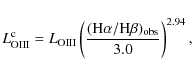
which assumes an intrinsic Balmer decrement equal to 3.0 as expected in the NLR (see Osterbrock & Ferland 2006).

In Fig. 1 (top panel) the distribution of the ratio between the (2-10) keV luminosity and the extinction-corrected [OIII] luminosity for our sample is shown. The mean of this distribution is

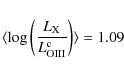
$\begin{displaymath} \langle \log \left( \frac{L_{\rm X}}{L^{\rm c}_{\rm OIII}} \right)\rangle=1.09 \end{displaymath}$

(2)

and the dispersion is 0.63 dex.

$\begin{figure} \par\includegraphics[width=7cm,clip]{12023f1a.ps}\vspace*{1.5mm} \includegraphics[width=7cm,clip]{12023f1b.ps} \end{figure}$	Figure 1: Distribution of log( $L_{\rm X}$ / $L^{\rm c}_{\rm OIII}$ ) (top) and log $L_{\rm X}$ -log $L^{\rm c}_{\rm OIII}$ relation (bottom). The solid line is the best-fit relation Eq. (3) for the 61 sources from Mulchaey et al. (1994) (crosses), B99 (squares), and P06 (triangles), while the dotted line is the best-fit relation obtained by P06.
Open with DEXTER

The bottom panel of Fig. 1 shows $L_{\rm X}$ versus L $^{\rm c}_{\rm OIII}$ . The correlation is highly significant (Spearman rank correlation coefficient $\rho=0.86$ , $P=1.6\times10^{-18}$ ). To quantify any distance-driven effects that may be present in a luminosity-luminosity correlation, we also performed a ``scrambling test'' (see e.g. Bregman 2005; Merloni et al. 2006; Bianchi et al. 2009b). The correlation does not appear to be affected by distance effects: not even a data-set out of the 100 000 simulated ones has a correlation coefficient as large as the one measured in the real data set.

An ordinary least-square bisector procedure gives the following best fit:

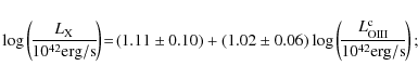
$\begin{displaymath} \log\left(\!\frac{L_{\rm X}}{10^{42}{\rm erg/s}}\!\right)\!=... ...ft(\!\frac{L^{\rm c}_{\rm OIII}}{10^{42}{\rm erg/s}}\!\right); \end{displaymath}$

(3)

i.e., we found a linear correlation between $L_{\rm X}$ and $L^{\rm c}_{\rm OIII}$ .

P06 investigated the same correlation finding that $L_{\rm X}$ $\propto$ L $^{\rm c}_{\rm OIII}$ $^{(1.22 \pm 0.06)}$ . They included in their analysis type 1 AGN, type 2 AGN, and Compton-thick sources (in the latter case they assumed that the intrinsic X-ray luminosity is 60 times higher than the observed one) and covered about five orders of magnitude in both [OIII] luminosity and X-ray luminosity. It should be recalled that the P06 sample is optically selected, while our sample, mainly based on the B99 catalogue, includes both optically selected and X-ray selected AGN. As discussed in several papers, most recently in Heckman et al. (2005) and Netzer et al. (2006, N06 hereafter), X-ray selected samples are likely to be biased towards X-ray bright sources, hence produce a higher X/[OIII] ratio compared to optically selected ones. The 44 sources that we have selected from the B99 catalogue all have log $L^{\rm c}_{\rm OIII} >39.3$ . The presence of X-ray selected objects among these sources should therefore tend to make the $L_{\rm X}$ -L $^{\rm c}_{\rm OIII}$ relationship steeper than found by P06, which, as can also be seen in Fig. 1, is exactly the opposite of what we found.

On the other hand, the high-luminosity ranges in P06 are nearly completely populated by type 1 AGN, for which we consider the estimate of $L^{\rm c}_{\rm OIII}$ unreliable. The steeper slope of the $L_{\rm X}$ - $L^{\rm c}_{\rm OIII}$ relation found by P06 could indeed stem from an underestimate of the reddening in these AGN types.

N06 studied the relation between $L_{\rm OIII}$ and $L_{\rm X}$ in samples of type 1 and type 2 AGN. They found that the ratio between $L_{\rm OIII}$ and $L_{\rm X}$ decreases with $L_{\rm X}$ , and the same result was obtained also for type 2 AGN using the extinction-corrected [OIII] luminosity. In that case, they used the B99 catalogue but excluded sources with optical classification ${\le}1.5$ and Compton-thick sources. They found log( $L^{\rm c}_{\rm OIII}$ / $L_{\rm X}$ ) = ( $15.0\pm4.0$ ) - ( $0.38\pm0.09$ )log $L_{\rm X}$ , which implies $L_{\rm X}$ $\propto$ $L^{\rm c}_{\rm OIII}$ ^1.61, i.e. a correlation with an even steeper slope than that obtained by P06. Our analysis only differs from N06 for the inclusion of the AGN optically classified as type 1.5. Excluding these sources from our sample, we found for the remaining 52 sources: $\log(L_{\rm X}/10^{42}{\rm erg/s})=(1.08\pm0.11)+(1.04\pm0.06)\log(L^{\rm c}_{\rm OIII}/10^{42}{\rm erg/s})$ ( $\rho$ = 0.85, $p=2.0\times 10 ^{-15}$ ), i.e. a significant linear correlation also in this case. The discrepancy between the results may come from the narrower range of luminosities covered by N06, which does not include sources with $L_{\rm X} \le$ 10⁴⁰erg/s. Unfortunately we cannot make a clear comparison with N06, because they did not perform a simple $L_{\rm X}$ - $L^{\rm c}_{\rm OIII}$ fit, an extrapolation of the resulting slope from their fit may be misleading. Moreover N06 did not explicitly report the method they used to compute the linear regression and the significance of the correlation they found.

The relation between $L_{\rm X}$ and L $^{\rm c}_{\rm OIII}$ can be combined with the X-ray bolometric correction (XBC) to obtain the [OIII] bolometric correction factor, $C_{\rm OIII}$ . Adopting the luminosity-dependent XBC of Marconi et al. (2004), we found a mean value of $C_{\rm OIII}$ in the luminosity ranges log $L_{\rm OIII}=38{-}40$ , 40-42, and 42-44 of 87, 142, and 454, respectively.

As a cautionary remark, it must be noted that the XBC may suffer from large uncertainties.

Marconi et al. (2004) and Hopkins et al. (2007) accounted for variations in AGN SEDs with luminosity using the anti-correlation between the optical-to-X-ray spectral index ( $\alpha_{\rm OX}$ ) and the luminosity at 2500 $\AA$ (L₂₅₀₀) (e.g. Vignali et al. 2003a), but Hopkins et al. (2007) find that the intrinsic spread in AGN SEDs could give rise to variation of a factor of $\sim$ 2 in the XBC, even when luminosity dependence is taken into account.

Moreover, the very dependence on luminosity of the X-ray bolometric correction has been questioned by Vasudevan & Fabian (2007), who estimate it from the observed SEDs of 54 AGNs. They find evidence of a large scatter in the XBC, with no simple dependence on luminosity, and suggest instead the Eddington ratio as the physical quantity the bolometric correction depends on.

Very recently, Kauffmann & Heckman (2009) have anticipated an estimate of $C_{\rm OIII}$ .

They find $C_{\rm OIII}$ in the range $\sim$ 500 to 800. Because the details of their analysis have not been published yet, for the time being we are not able to discuss the origin of this discrepancy.

3 The Eddington ratio distribution of type 2 SDSS AGN at 0.3 <z< 0.4

B06 measured the stellar velocity dispersion, $\sigma_{\ast}$ , for 30 sources of the 0.3<z<0.8 SDSS type 2 AGN sample of Zakamska et al. (2003). The stellar velocity dispersion was obtained by fitting the profile of heavy element absorption lines, which are mainly associated with the old stellar population in the bulge. Then, they estimated the black hole masses from $\sigma_{\ast}$ , adopting the Tremaine et al. (2002) relation.

The B06 subsample is representative of the total sample of Zakamska et al. (2003) with respect to $L_{\rm OIII}$ . Indeed, the observation of significant stellar absorption features, which is the key point in accurately measuring $\sigma_{\ast}$ , does not appear to depend on the nuclear luminosity of the sources, as confirmed by a t-test (see B06).

For 15 sources, B06 calculated the [OIII] line luminosity corrected for extinction using the observed Balmer decrement and Eq. (1). Therefore all these sources have $z \leq 0.4$ , because of the limited wavelength coverage of the SDSS spectroscopy ( $\simeq$ 3800-9200 $\AA$ ). The ratio between $L^{\rm c}_{\rm OIII}$ and $L_{\rm OIII}$ is between 0.6 and 17.8. The observed Balmer decrement is lower in three objects than the theoretical value, most likely due to an imperfect subtraction of the starlight. We assigned zero extinction to these objects.

Figure 4 in B06 shows the distribution of the Eddington ratios of the 15 sources where we have a reliable estimate of $L^{\rm c}_{\rm OIII}$ . This distribution is surprising for its mean value, $\langle \lambda \rangle$ $\simeq$ 1; because it would reveal a population of high Eddington ratio sources that are not observed in the local Universe, such Eddington ratios are neither observed in type 1 AGN at higher redshift.

However, it is important to note that B06 obtained this distribution by estimating the bolometric luminosity from $L^{\rm c}_{\rm OIII}$ and the BC given by H04. This bolometric correction applies to $L_{\rm OIII}$ and not to $L^{\rm c}_{\rm OIII}$ , therefore B06 overestimated $L_{\rm b}$ in a systematic manner and hence $\lambda$ .

In this section we use $C_{\rm OIII}$ , as computed in Sect. 2, to calculate the Eddington ratio distribution of the type 2 SDSS AGN of the B06 sample. First of all we have tested the reliability of deriving $\lambda$ from the [OIII] line luminosity in an optically selected sample, adopting the $C_{\rm OIII}$ we derived in a collection of X-ray selected and optically selected sources. To this aim we used the P06 subsample used in Sect. 2. In the top panel of Fig. 2 the Eddington ratio estimates obtained from $L^{\rm c}_{\rm OIII}$ and $C_{\rm OIII}$ ( $\lambda _{\rm OIII}$ ) are compared with those obtained from $L_{\rm X}$ and the XBC of Marconi et al. (2004, $\lambda _{\rm X}$ ; the black hole masses taken from Table 2 of P06). We find good agreement between the X-ray and the [OIII] estimates.

For the 8 SDSS AGN of the B06 sample for which we have XMM-Newton observations, we can repeat the above check. The bottom panel of Fig. 2 shows $\lambda _{\rm X}$ versus $\lambda _{\rm OIII}$ obtained from $L^{\rm c}_{\rm OIII}$ and $C_{\rm OIII}$ and versus $\lambda _{\rm OIII}$ obtained by B06. As expected, the $\lambda _{\rm OIII}$ obtained by B06 are systematically larger than those derived from the X-ray luminosity, while this effect disappears when the proper bolometric correction is used.

The black hole mass, the [OIII] line luminosity, the extinction-corrected [OIII] line luminosity, the (2-10) keV observed flux ( $F^{\rm obs}_{\rm X}$ ), and the intrinsic (i.e. de-absorbed) (2-10) keV luminosity ( $L^{\rm int}_{\rm X}$ ) of the X-ray observed sources are listed in Table 1. The X-ray data reduction and the estimate of $L^{\rm int}_{\rm X}$ either from X-ray spectral fitting or extrapolated from the observed X-ray count rates (or upper limits) are reported in the Appendix. The [OIII] luminosities are derived from the SDSS spectra, except for SDSSJ083945.98+384319.0. This source has z=0.424 so the SDSS spectrum does not cover the spectral range necessary to measure the H $\alpha$ line. The [OIII] line luminosity and the Balmer decrement measurements are obtained from observation collected with the 2.2 m telescope at the Centro Astronómico Hispano Alemán (CAHA) at Calar Alto.

$\begin{figure} \par\includegraphics[width=7.5cm,clip]{12023f2a.ps}\vspace*{1.5mm} \includegraphics[width=7.5cm,clip]{12023f2b.ps} \end{figure}$	Figure 2: Top: $\lambda _{\rm X}$ vs. $\lambda _{\rm OIII}$ for the sources in the P06 subsample. Bottom: $\lambda _{\rm X}$ vs. $\lambda _{\rm OIII}$ obtained by B06 (squares) and from $L^{\rm c}_{\rm OIII}$ and $C_{\rm OIII}$ (crosses), for the B06 sources with the XMM- Newton observations.
Open with DEXTER

Table 1: Properties of the SDSS type 2 AGN

Figure 3 shows the $\lambda$ -distribution of the B06 sample obtained using $L^{\rm c}_{\rm OIII}$ and $C_{\rm OIII}$ to estimate the bolometric luminosity. This distribution is obviously shifted to lower $\lambda$ values with respect to that obtained by B06: the mean of this distribution is $\langle \lambda \rangle \simeq 0.1$ , a value that is similar to that estimated in other AGN samples.

We have checked whether the width of the observed $\lambda$ -distribution indicates a physical spread in the Eddington ratios or can be due to the dispersion in the $L^{\rm c}_{\rm OIII}$ - $L_{\rm b}$ relation. In practice, we checked that the observed distribution is consistent with a log-normal distribution centred at log $\lambda=-1$ and with width equal to the dispersion in the $L_{\rm X}$ - $L^{\rm c}_{\rm OIII}$ relation (0.63 dex). A Kolmogorov-Smirnov test gives D=0.27, which corresponds to a probability of 0.18 for the null hypothesis that the two distributions are drawn from the same parent population.

$\begin{figure} \par\includegraphics[width=7.3cm,clip]{12023f3.ps} \end{figure}$	Figure 3: Eddington ratio distribution of the B06 sample, which is obtained by estimating $\lambda$ from $L^{\rm c}_{\rm OIII}$ and $C_{\rm OIII}$ .
Open with DEXTER

4 Conclusions

In this paper we estimate the bolometric correction factor, $C_{\rm OIII}$ , needed to convert the extinction-corrected [OIII] line luminosity to bolometric luminosity.

We determined $C_{\rm OIII}$ in a two-step process. First we studied the $L_{\rm X}$ - $L^{\rm c}_{\rm OIII}$ relation in a sample of 61 Seyfert galaxies with reliable measurements of both $L^{\rm c}_{\rm OIII}$ and $L_{\rm X}$ ; i.e., we selected galaxies with reliable measurement of the Balmer decrement (Seyfert galaxies with optical classification $\ge$ 1.5) and X-ray Compton-thin sources. The bolometric correction C $_{\rm OIII}$ was then obtained by combining the mean ratio between $L_{\rm X}$ and $L^{\rm c}_{\rm OIII}$ with the luminosity-dependent X-ray bolometric correction of Marconi et al. (2004). We found a mean value of C $_{\rm OIII}$ in the luminosity ranges log $L_{\rm OIII}=38{-}40$ , 40-42, and 42-44 of 87, 142, and 454, respectively.

Similarly, H04 estimated the [OIII] bolometric correction by combining the mean ratio between L₅₀₀₀ and $L_{\rm OIII}$ in a sample of type 1 AGN with the 5000 Angstrom continuum to $L_{\rm bol}$ correction from Marconi et al. (2004). H04 did not correct $L_{\rm OIII}$ for the extinction in the NLR, therefore their bolometric correction applies to the ``observed'' [OIII] luminosities. Compared to H04 our estimate of the [OIII] bolometric correction is not subject from the scatter due to the extinction in the NLR, which we estimated to be about 0.6 dex from our sample.

The [OIII] line luminosity is an indirect estimator of the nuclear luminosity, depending on the geometry of the system, and on any possible shielding effect that may affect the ionizing radiation seen by the NLR. The amount of gas that is exposed to the ionizing radiation depends on the torus opening angle. Bianchi et al. (2007, and references therein) confirmed the Iwasawa-Taniguchi (IT) effect, i.e. the anti-correlation between the iron line equivalent width and the X-ray luminosity. The simplest explanation for the IT effect is in terms of a decrease in the torus covering factor (and hence an increase in its opening angle) with luminosity, which may also explain the observed decrease with luminosity of the ratio between mid-IR and bolometric luminosities (Maiolino et al. 2007; Treister et al. 2008). If this explanation is correct, we would expect a less than linear relation between $L_{\rm X}$ and $L^{\rm c}_{\rm OIII}$ , different from what we found. The situation is even worse with the more than linear relations found by P06 and N06. This problem will be addressed in a forthcoming paper.

We used $C_{\rm OIII}$ to estimate the Eddington ratio distribution of type 2 SDSS AGN at 0.3<z<0.4 from the B06 sample. B06 find that the mean of this distribution is $\langle \lambda \rangle \simeq$ 1, thus revealing a population of high Eddington ratio sources that is absent in the local Universe and in type 1 AGN at higher redshift (e.g. Woo & Urry 2002; McLure & Dunlop 2004; Warner et al. 2004; Kollmeier et al. 2006; Vestergaard 2002, 2004; Netzer & Trakhtenbrot 2007). However, we have demonstrated, with the help of the X-ray luminosities, that B06 have sistematically overestimated the bolometric luminosities, hence the Eddington ratios, which we found to be $\langle \lambda \rangle \simeq 0.1$ , similar to what is found in other AGN samples.

Acknowledgements

This work benefitted from an Italy-Spain Integrated Actions, reference HI-0079. A.L., G.M., and S.B. acknowledge financial support from ASI (grant I/088/06/0). X.B. and F.J.C. acknowledge financial support by the Spanish Ministerio de Ciencia e Innovación under project ESP2006-13608-C02-01. The authors thank Cristian Vignali for useful discussions, and the anonymous referee for constructive comments. The work is based on observations obtained with XMM-Newton, an ESA science mission with instruments and contributions directly funded by ESA Member States and the USA (NASA), and on observation collected with the 2.2 m telescope at the Centro Astronómico Hispano Alemán (CAHA) at Calar Alto, operated jointly by the Max-Planck Institut für Astronomie and the Instituto de Astrofísica de Andalucía (CSIC).

Appendix A: The X-ray data

Table A.1: X-ray count rates.

Of the 8 sources presented in this paper, 7 were observed as a part of our XMM-Newton proposal ID 050206 and ID 055120, and one was observed serendipitously. The data were processed using the XMM-Newton Science Analysis Software (SAS) v.8.0. The raw event files (the Observation Data Files, ODF), have been linearized with the XMM-SAS pipeline EPPROC for the PN camera, and we generated calibration files using the XMM-SAS pipeline CIFBUILD. Event files were cleaned from bad pixel (hot pixels and events out of the field of view), and we selected events spread at most in two contiguous pixels (pattern = 0-4). We removed periods of high background levels by analysing the light curves of the count rate at energies higher than 10 keV. Response functions (the ancillary response file and the redistribution matrix file) for spectral fitting were generated using the SAS tasks RMFGEN and ARFGEN. We extracted the PN counts in a circular region with radius of 15^'', centred at the source position, and the background counts in the source-free regions close to the target.

The SDSS name, redshift, exposure times (filtered for good time intervals), and X-ray PN count rates (or 5 $\sigma$ upper limits) in the rest frame energy ranges (0.5-2) keV and (2-10) keV are listed in Table A.1.

Of the 8 sources, two are detected (i.e. the Poisson probability of a spurious background excess is less than 2.7 $\times$ 10^-3) in the (0.5-10) keV band, two only in the soft band (0.5-2 keV) and one only in the hard band (2-10 keV).

Sufficient counts for a spectral fitting in the 2-10 keV band were only collected from three sources: SDSSJ075920.21+351903.4, SDSSJ143928.23+001538.0, and SDSSJ083945.98+384319.0.

Spectral analysis was carried out with XSPEC v.12.4.0 using data accumulated in energy bins with 5 counts each and the C-statistic (Cash 1979). The spectral fits are shown in Fig. A.1.

The X-ray spectra in the (0.5-10) keV band are fitted with an absorbed power-law continuum plus a Compton-reflection component and a soft-excess component, modelled with a power-law with photon index equal to the one of the primary continuum. The parameters of the fits along with the observed (2-10) keV flux, and the de-absorbed (2-10) keV luminosity are shown in Table A.2. In SDSSJ075920.21+351903.4 an iron line with equivalent width of about 2.6 keV is also detected, revealing that this source is Compton-thick. In these sources the primary X-ray emission is totally suppressed below 10 keV, the hard X-ray emission is accounted for by reflection of the primary nuclear emission off the inner walls of optically thick circumnuclear matter.

Table A.2: Best-fit parameters.

The luminosity reported in Table A.2 is obtained assuming that the ratio between the reflected and the primary component is 0.05, similar to what is observed in the Circinus galaxy, one of the best-studied Compton-thick sources (Matt et al. 1999).

The upper limits in the X-ray luminosity, listed in Table 1, for the other sources are extrapolated from the observed count rates (Col. 5 of Table A.1) assuming a typical spectrum of Compton-thick sources. The spectrum is assumed to be a power law with photon index $\Gamma=1.9$ absorbed by column density of $N_{\rm H}=1.5\times 10^{24}$ , plus a pure Compton reflection component with an iron line (at 6.4 keV and with equivalent width EW=1 keV with respect of the pexrav component). The ratio between the reflected and the primary component is assumed to be 0.05. We chose this spectrum because we wanted to study the extreme case of obscuration that implies the higher intrinsic X-ray luminosities and therefore the higher bolometric luminosities.

$\begin{figure} \par\includegraphics[width=6.5cm,angle=270,clip]{12023f4.ps}\vspa... ...ce*{1.5mm} \includegraphics[width=6.5cm,angle=270,clip]{12023f6.ps} \end{figure}$	Figure A.1: XMM- Newton spectra of SDSSJ083945.98+384319.0, SDSSJ143928.23+001538.0, and SDSSJ075920.21+351903.4 from top to bottom.
Open with DEXTER

We used this method to also estimate $L^{\rm int}_{\rm X}$ in the sources detected only in the soft band, because from the comparison between the observed X-ray luminosity and that predicted from $L^{\rm c}_{\rm OIII}$ and Eq. (2), we argued that they are heavily absorbed sources. Therefore the soft X-ray emission is not the primary soft X-ray emissions but a soft excess component.

References

Antonucci, R. R. J. 1993, ARA&A, 31, 473 [NASA ADS] (In the text)
Bassani, L., Dadina, M., Maiolino, R., et al. 1999, ApJS, 121, 473 [NASA ADS] [CrossRef] (B99) (In the text)
Bentz, M. C., Peterson, B. M., Pogge, R. W., Vestergaard, M., & Onken, C. A. 2006, ApJ, 644, 133 [NASA ADS] [CrossRef] (In the text)
Bian, W., Gu, Q., Zhao, Y., Chao, L., & Cui, Q. 2006 MNRAS 372, 876 (B06) (In the text)
Bianchi, S., Guainazzi, M., Matt, G., & Fonseca Bonilla, N. 2007, A&A, 467, L19 [NASA ADS] [CrossRef] [EDP Sciences] (In the text)
Bianchi, S., Corral, A., Panessa, F., et al. 2008, MNRAS, 385, 195 [NASA ADS] [CrossRef] (In the text)
Bianchi, S., Guainazzi, M., Matt, G., Fonseca Bonilla, N., & Ponti, G. 2009a, A&A, 495, 421 [NASA ADS] [CrossRef] [EDP Sciences]
Bianchi, S., Fonseca Bonilla, N., Guainazzi, M., Matt, G., & Ponti, G. 2009b, A&A, 501, 915 [NASA ADS] [CrossRef] [EDP Sciences] (In the text)
Bregman, J. N. 2005 [arXiv:astro-ph/0511368] (In the text)
Ferrarese L., & Merritt, D. 2000, ApJ, 539, L9 [NASA ADS] [CrossRef] (In the text)
Gebhardt, K., Kormendy, J., Ho, L. C., et al. 2000a, ApJ, 539, L13 [NASA ADS] [CrossRef] (In the text)
Heckman, T., Kauffmann, G., Brinchmann, J., et al. 2004, ApJ, 613, 109 [NASA ADS] [CrossRef] (H04) (In the text)
Heckman, T. M., Ptak, A., Hornschemeier, A., & Kauffmann, G. 2005, ApJ, 634, 161 [NASA ADS] [CrossRef] (In the text)
Hopkins, P. F., Richards, G. T., & Hernquist, L. 2007, ApJ, 654, 731 [NASA ADS] [CrossRef] (In the text)
Kaspi, S., Smith, P. S., Netzer, H., et al. 2000, ApJ, 533, 631 [NASA ADS] [CrossRef] (In the text)
Kaspi, S., Maoz, D., Netzer, H., et al. 2005, ApJ, 629, 61 [NASA ADS] [CrossRef] (In the text)
Kauffmann, G., Heckman, T. M., Tremonti, C., et al. 2003b, MNRAS, 346, 1055 [NASA ADS] [CrossRef] (In the text)
Kauffmann, G., & Heckman, T. M., 2009, MNRAS, 397, 135 [NASA ADS] [CrossRef] (In the text)
Kollmeier, J. A., Onken, C. A., Kochanek, C. S., et al. 2005 ApJ, 648, 128
Magorrian, J., Tremaine, S., Richstone, et al. 1998, AJ, 115 2285 (In the text)
Maiolino, R., Shemmer, O., Imanishi, M., et al. 2007, A&A, 468, 979 [NASA ADS] [CrossRef] [EDP Sciences]. (In the text)
Marconi, A., Risaliti, G., Gilli, R., et al. 2004, MNRAS, 351, 169 [NASA ADS] [CrossRef] (In the text)
Matt, G., Guainazzi, M., Maiolino, R., et al. 1999, A&A 341, L39 (In the text)
McLure, R. J., & Dunlop, J. S. 2004, MNRAS, 352, 1390 [NASA ADS] [CrossRef] (In the text)
Menci, N., Cavaliere, A., Fontana, A., et al. 2003, ApJ, 587, L63 [NASA ADS] [CrossRef] (In the text)
Menci, N., Fiore, F., Perola, G. C., & Cavaliere, A. 2004, ApJ, 606, 58 [NASA ADS] [CrossRef] (In the text)
Merloni, A., Körding, E., Heinz, S., et al. 2006, NewA, 11, 567 [NASA ADS] [CrossRef] (In the text)
Mulchaey, J. S., Koratkar, A., Ward, M. J., et al. 1994, ApJ, 436, 586 [NASA ADS] [CrossRef] (In the text)
Netzer, H., & Trakhtenbrot, B. 2007, ApJ, 654, 754 [NASA ADS] [CrossRef] (In the text)
Netzer, H., Mainieri, V., Rosati, P., & Trakhtenbrot, B. 2006, A&A, 453, 525 [NASA ADS] [CrossRef] [EDP Sciences] (N06) (In the text)
Osterbrock, D. E., & Ferland, G. J. 2006, Book Review: Astrophysics of Gaseous Nebulae and ACtive Galactic Nuclei, 2edn. (University Science Books) (In the text)
Panessa, F., Bassani, L., Cappi, M., et al. 2006, A&A 455, 173 (P06)
Peterson, B. M., Ferrarese, L., Gilbert, K. M., et al. 2004, ApJ, 613, 682 [NASA ADS] [CrossRef] (In the text)
Peterson, B. M., Bentz, M. C., Desroches, L. B., et al. 2005, ApJ, 632, 799 [NASA ADS] [CrossRef] (In the text)
Treister E., Krolik J. H., & Dullemond C. 2008, ApJ, 679, 140 [NASA ADS] [CrossRef] (In the text)
Tremaine, S., Gebhardt, K., Bender, R., et al. 2002, ApJ, 574, 740 [NASA ADS] [CrossRef] (In the text)
Vasudevan, R. V., & Fabian, A., 2007 MNRAS, 381, 1235 (In the text)
Vestergaard, M. 2002, ApJ, 571, 733 [NASA ADS] [CrossRef] (In the text)
Vestergaard, M. 2004, ApJ, 601, 676 [NASA ADS] [CrossRef] (In the text)
Vignali, C., Brandt, W. N., & Schneider, D. P. 2003, AJ, 125, 433 [NASA ADS] [CrossRef] (In the text)
Warner, C., Hamann, F., & Dietrich, M. 2004, ApJ, 608, 136 [NASA ADS] [CrossRef] (In the text)
Woo, J., & Urry, C. M. 2002, ApJ, 579, 530 [NASA ADS] [CrossRef] (In the text)
Zakamska, N. L., Strauss, M. A., Krolik, J. H., et al. 2003, AJ, 126, 2125 [NASA ADS] [CrossRef] (In the text)

Footnotes

...1994): We used $L_{\rm OIII}$ and Balmer decrement from Mulchaey et al. (1994) and the X-ray luminosities from Bianchi et al. (2009a).
... significant: We consider those correlations statistically significant whose null hypothesis probability, P, are lower than 1 $\times$ 10^-3, which correspond to a confidence level of 99.9 $\%$ .

All Tables

Table 1: Properties of the SDSS type 2 AGN

Table A.1: X-ray count rates.

Table A.2: Best-fit parameters.

All Figures

$\begin{figure} \par\includegraphics[width=7cm,clip]{12023f1a.ps}\vspace*{1.5mm} \includegraphics[width=7cm,clip]{12023f1b.ps} \end{figure}$	Figure 1: Distribution of log( $L_{\rm X}$ / $L^{\rm c}_{\rm OIII}$ ) (top) and log $L_{\rm X}$ -log $L^{\rm c}_{\rm OIII}$ relation (bottom). The solid line is the best-fit relation Eq. (3) for the 61 sources from Mulchaey et al. (1994) (crosses), B99 (squares), and P06 (triangles), while the dotted line is the best-fit relation obtained by P06.
Open with DEXTER
In the text

$\begin{figure} \par\includegraphics[width=7.5cm,clip]{12023f2a.ps}\vspace*{1.5mm} \includegraphics[width=7.5cm,clip]{12023f2b.ps} \end{figure}$	Figure 2: Top: $\lambda _{\rm X}$ vs. $\lambda _{\rm OIII}$ for the sources in the P06 subsample. Bottom: $\lambda _{\rm X}$ vs. $\lambda _{\rm OIII}$ obtained by B06 (squares) and from $L^{\rm c}_{\rm OIII}$ and $C_{\rm OIII}$ (crosses), for the B06 sources with the XMM- Newton observations.
Open with DEXTER
In the text

$\begin{figure} \par\includegraphics[width=7.3cm,clip]{12023f3.ps} \end{figure}$	Figure 3: Eddington ratio distribution of the B06 sample, which is obtained by estimating $\lambda$ from $L^{\rm c}_{\rm OIII}$ and $C_{\rm OIII}$ .
Open with DEXTER
In the text

$\begin{figure} \par\includegraphics[width=6.5cm,angle=270,clip]{12023f4.ps}\vspa... ...ce*{1.5mm} \includegraphics[width=6.5cm,angle=270,clip]{12023f6.ps} \end{figure}$	Figure A.1: XMM- Newton spectra of SDSSJ083945.98+384319.0, SDSSJ143928.23+001538.0, and SDSSJ075920.21+351903.4 from top to bottom.
Open with DEXTER
In the text

Current usage metrics show cumulative count of Article Views (full-text article views including HTML views, PDF and ePub downloads, according to the available data) and Abstracts Views on Vision4Press platform.

Data correspond to usage on the plateform after 2015. The current usage metrics is available 48-96 hours after online publication and is updated daily on week days.

Initial download of the metrics may take a while.