| Issue |
A&A
Volume 503, Number 3, September I 2009
|
|
|---|---|---|
| Page(s) | 683 - 690 | |
| Section | Astrophysical processes | |
| DOI | https://doi.org/10.1051/0004-6361/200912217 | |
| Published online | 09 July 2009 | |
Nonlinear electrostatic modes in astrophysical plasmas with charged dust distributions
F. Verheest1,2 - V. V. Yaroshenko3
1 - Sterrenkundig Observatorium, Universiteit Gent, Krijgslaan 281, 9000 Gent, Belgium
2 -
School of Physics, University of KwaZulu-Natal, Private Bag X54001, Durban 4000, South Africa
3 -
Max-Planck-Institut für extraterrestrische Physik, 85741 Garching, Germany
Received 27 March 2009 / Accepted 2 June 2009
Abstract
Context. Most theoretical investigations of wave phenomena in dusty plasmas have treated charged dust as additional heavy negative ions in standard multispecies models. Many dusty plasma experiments use monodisperse grains, but charged (and neutral) grains in space environments come in a whole range of sizes and compositions, hence in masses and charges. Dust density distributions having a power-law decay with size are often observed in planetary rings.
Aims. There is a need to investigate larger solitary structures, since wave descriptions involving charged dust distributions have usually been limited to linear or weakly nonlinear modes.
Methods. Sagdeev pseudopotential methods describe large-amplitude solitary waves in a co-moving reference frame and are adapted to include dust distributions, using mass and charge, or alternatively size, as additional variables. Observed power-law distributions lead to descriptions involving hypergeometric functions.
Results. Lower limits for possible solitary wave velocities follow from requiring that the Sagdeev pseudopotentials have a local maximum for the undisturbed conditions, whereas upper limits come from ensuring that dust densities remain real. Nonlinear amplitudes increase with solitary wave velocities and relative electron temperature. Under similar plasma conditions, dust size distributions admit slower solitary wave solutions, with correspondingly smaller amplitudes than given by monodisperse dust models. For typical planetary ring conditions, the difference can be quite appreciable.
Key words: plasmas - waves - planets: rings
1 Introduction
This paper combines two strands of current research in the description of space and astrophysical plasmas. On the one hand, there is the continuing modeling of exact large scale nonlinear solitary waves for many different plasma compositions, on which a vast literature has sprung up since the pioneering work by Sagdeev (1966). Only some immediately relevant references will be given below, there being no hope of doing this extended domain any semblance of justice. Solitary waves seen in space have usually been in the form of bipolar pulses in the electric field or humps and dips in the electrostatic potential and observed in many parts of the magnetosphere: for instance, the auroral region (Bounds et al. 1999), the bow shock (Bale et al. 1998), the magnetosheath (Pickett et al. 2003), and the plasma sheet boundary region (Matsumoto et al. 1994; Frantz et al. 1998), to quote just a selected few.
On the other hand, the theoretical treatment of wave phenomena in dusty plasmas (see, e.g., monographs by Bliokh et al. 1995; Verheest 2000; Shukla & Mamun 2002) has mostly introduced charged dust as heavy negative ion species, in models that are extensions of earlier work on more usual plasmas. While many dusty plasma experiments have used manufactured monodisperse grains, charged (and neutral) grains in space and astrophysical situations come in a whole range of sizes and compositions, hence also masses and charges. Moreover, in situ observations of planetary environments by space missions have often shown that dust distributions are characterized by power-law decays of dust densities with size (Gurnett et al. 1983; Showalter et al. 1992; Showalter & Cuzzi 1993; Kempf et al. 2006; Kurth et al. 2006; Kempf et al. 2008; Yaroshenko et al. 2009).
Incorporating the effect of charged dust distributions in the description of waves in dusty plasmas has mostly been restricted to linear or weakly nonlinear modes (Tripathi & Sharma 1996; Meuris et al. 1997; Brattli et al. 1997; de Juli & Schneider 1998; Yaroshenko et al. 2001), so we describe large-amplitude, nonlinear solitary waves in space plasmas that contain charged dust distributions, to which end we have to adapt the Sagdeev pseudopotential formalism.
The plan of the paper is as follows. After this introduction, Sect. 2 shows how dust distributions within a range of charges and masses can be dealt with in a Sagdeev pseudopotential formalism, which is specialized in Sect. 3 to grain size distributions with a power-law decay, as often observed in space plasmas. Weakly nonlinear solitary structures is looked at in Sect. 4, whereas Sect. 5 treats the fully nonlinear case and delimits the existence ranges in compositional parameter space in terms of physical concepts. A comparison is then made with monodisperse dust descriptions in Sect. 6, and Sect. 7 sums up our conclusions.
2 Nonlinear formalism
First we very briefly repeat some of the steps needed to describe complex plasmas with polydisperse charged dust, with emphasis on a methodologically correct way. We distinguish between the electrons and ions treated by standard theory, on the one hand, and the dust distributions, described by appropriate integrals over the charge and mass distributions, on the other.
For electrostatic problems, the waves are longitudinal, so that only scalar velocities are needed.
To avoid all ambiguities, we start from a microscopic distribution function
![]() for the dust in phase space, which incorporates the dust charge q and the mass m as continuous, independent microscopic phase space variables, besides x, t, and the phase space parallel velocity w. This is governed by an extended Vlasov-type kinetic equation
(Verheest et al. 2002a; Verheest & Cattaert 2004b,a; Verheest et al. 2003; Varma 2000), which for electrostatic modes reads as
for the dust in phase space, which incorporates the dust charge q and the mass m as continuous, independent microscopic phase space variables, besides x, t, and the phase space parallel velocity w. This is governed by an extended Vlasov-type kinetic equation
(Verheest et al. 2002a; Verheest & Cattaert 2004b,a; Verheest et al. 2003; Varma 2000), which for electrostatic modes reads as
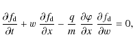
where the microscopic laws of motion
After multiplication with some power of the microscopic velocities, integration of ( In the text 1) over all q, m and w yields the traditional chain of moment equations in physical space for one-dimensional motion. As explained elsewhere (Verheest & Cattaert 2003), different charge and mass weightings compel one to introduce a whole sequence of velocities and higher order moments, where the same order in w is combined with different powers of q and m. To avoid these complications, we postpone the integration over the new phase space variables q and m and restrict ourselves first to integrations solely over the microscopic velocity w.
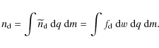
More details about this half-way house procedure are given elsewhere (Verheest & Cattaert 2004b,a), and, in this sense, we define the zeroth velocity moment of ![]() as
as
 |
(2) |
such that the real physical dust density obtains as
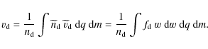
In this intermediate description, variables will be indicated with a tilde, to show that these still contain variable q and m, integrations over which have to be carried out at a later stage. As
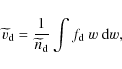 |
(4) |
such that the dust fluid velocity is given by
Hence, the first moment equations for the dust are similar to the continuity and momentum equations for ordinary plasma species, but with a different interpretation, because q and m are variable. We start from
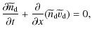
written for cold dust, without pressure effects.
We use the stationary form (
![]() )
of the equation of continuity (6) and motion (7), to get first integrals expressing mass flux and momentum conservation, as it is easier to work in the wave frame moving with the nonlinear solitary structure. This change in reference frame entails a redefinition of the microscopic distribution functions
)
of the equation of continuity (6) and motion (7), to get first integrals expressing mass flux and momentum conservation, as it is easier to work in the wave frame moving with the nonlinear solitary structure. This change in reference frame entails a redefinition of the microscopic distribution functions ![]() in terms of the microscopic velocities.
in terms of the microscopic velocities.
Since in an inertial frame all species are macroscopically at rest in the absence of solitary structures, this holds for the cold dust for all q and m within the admissible ranges.
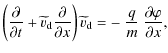
In the wave frame (6) expresses mass conservation as
| (8) |
where V is the velocity of the solitary wave as it would be seen in an inertial frame, but, in the wave frame, V corresponds to the undisturbed plasma velocities far away from the solitary wave. Hence we have also
 |
(9) |
Eliminating
The plasma electrons and ions will be described by the usual Boltzmann distributions,
![$\displaystyle n_{\rm e} = n_{\rm e0} \exp\left[\frac{e\varphi}{T_{\rm e}}\right],$](/articles/aa/full_html/2009/33/aa12217-09/img35.png)
![$\displaystyle n_{\rm i} = n_{\rm i0} \exp\left[-~\frac{e\varphi}{T_{\rm i}}\right],$](/articles/aa/full_html/2009/33/aa12217-09/img36.png)
with respective kinetic temperatures
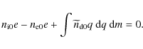
The basic description is closed by Poisson's equation,
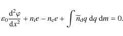
After multiplication by
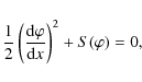
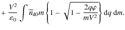
where the Sagdeev pseudopotential
![$\displaystyle \frac{n_{\rm e0} T_{\rm e}}{\varepsilon_0} \left(
1 - \exp\left[\frac{e\varphi}{T_{\rm e}} \right] \right)$](/articles/aa/full_html/2009/33/aa12217-09/img45.png)
![$\displaystyle +~ \frac{n_{\rm i0} T_{\rm i}}{\varepsilon_0} \left( 1 - \exp\left[
-~ \frac{e\varphi}{T_{\rm i}} \right] \right)$](/articles/aa/full_html/2009/33/aa12217-09/img46.png)
Now ( In the text 14) has the form of an energy integral in classical mechanics, for particles with unit mass in a conservative force field,
It is seen that S(0) and
![]() ,
and in order to have the possibility of solitary structures, we need the proper convexity in the origin, namely that
,
and in order to have the possibility of solitary structures, we need the proper convexity in the origin, namely that
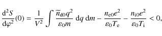
ensuring that the origin is a local maximum for
 |
(17) |
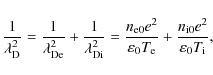
as well as the correct definition of the total dust plasma frequency
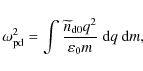
allows us to rewrite the so-called soliton condition (16) as
This requires possible solitary structures to be superacoustic with respect to the dust-acoustic velocity
Note that while this is a necessary condition, it is not sufficient to guarantee that solitary modes will exist. There are further restrictions on V that follow from the occurrence (or not) of roots for
![]() outside
outside ![]() .
.
3 Dust size distributions
For astrophysical plasmas, the main difficulties lie not so much in estimating ![]() and
and ![]() ,
but to know how the dust distributions
,
but to know how the dust distributions
![]() vary with q and m, and in what ranges. To simplify the general description and have a manageable discussion when dealing with planetary dust rings, we will assume in this section that we can use the size a of the dust grains as the variable factor.
vary with q and m, and in what ranges. To simplify the general description and have a manageable discussion when dealing with planetary dust rings, we will assume in this section that we can use the size a of the dust grains as the variable factor.
Now we assume that the dust grains all have equilibrium charges determined from the orbital-motion-limited (OML) or spherical probe charging theory (see, e.g., Bliokh et al. 1995; Verheest 2000; Shukla & Mamun 2002), where the dust is charged by electron and ion currents to the grains. For space dusty plasmas, which usually are weakly collisional, the OML theory represents a good approximation. Measurements of the particle charges made by the Cassini orbiter within Saturn's E-ring, e.g., are in quite reasonable agreement when compared to theoretical predictions based on the OML theory (Kempf et al. 2006).
In this model the dust charge is negative and proportional to the grain size a, in a given plasma environment. Furthermore, for grains composed of similar material the mass varies with a3.
Thus we can put
q(a) = - Q a and
m(a) = M a3, so that we are actually dealing with a dust size distribution and the (redefined) distribution function
![]() will now depend on a as the parameter characterizing the dust distribution, instead of on q and m separately.
will now depend on a as the parameter characterizing the dust distribution, instead of on q and m separately.
Next we take a standard power-law distribution, i.e. we assume that
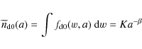
in an interval
Power-law density decreases with size, as in (20), are typical for different space plasma environments. Distributions of this sort have been observed in planetary ring plasmas, with power-law indices
![]() for the F ring of Saturn (Showalter et al. 1992) and
for the F ring of Saturn (Showalter et al. 1992) and ![]() (Showalter & Cuzzi 1993), or
(Showalter & Cuzzi 1993), or ![]() (Gurnett et al. 1983) for the G ring. The Voyager observations that have yielded these power-law indices and related information about planetary dust in the rings of the Jovian planets are more than two decades old. However exciting these observations may have been, they essentially
correspond to snapshots from the flybys of the Voyager spacecraft on their Grand Tour of the solar system.
(Gurnett et al. 1983) for the G ring. The Voyager observations that have yielded these power-law indices and related information about planetary dust in the rings of the Jovian planets are more than two decades old. However exciting these observations may have been, they essentially
correspond to snapshots from the flybys of the Voyager spacecraft on their Grand Tour of the solar system.
Hence the anticipation to more extended and precise data from the Cassini mission, which from the middle of 2004 onwards have reached us and which now confirm that dust size distributions are indeed well described by power laws. During most encounters with Saturn's rings in the vicinity of the icy moon Enceladus, the power law index inferred from dust impact measurements was found to be between
![]() (Kempf et al. 2008), while the Cassini Radio and Plasma Wave Science instrument predicted
(Kempf et al. 2008), while the Cassini Radio and Plasma Wave Science instrument predicted
![]()
![]() 1.0 (Kurth et al. 2006). Estimates based on Langmuir probe plasma measurements yielded even steeper dust distributions with
1.0 (Kurth et al. 2006). Estimates based on Langmuir probe plasma measurements yielded even steeper dust distributions with
![]() (Yaroshenko et al. 2009).
(Yaroshenko et al. 2009).
Moreover, for typical solar system dust size distributions the parameter
![]() is small enough to simplify some of the subsequent expressions for
is small enough to simplify some of the subsequent expressions for ![]() values between 4 and 7. Power-law distributions are fairly generic for other astrophysical plasmas, as in molecular clouds, based on considerations that smaller grains are more numerous than larger ones, although detailed observations outside the solar system are lacking for the time being.
values between 4 and 7. Power-law distributions are fairly generic for other astrophysical plasmas, as in molecular clouds, based on considerations that smaller grains are more numerous than larger ones, although detailed observations outside the solar system are lacking for the time being.
We find for the undisturbed dust charge density that
In accordance with observational results, we often will in this and the following expressions assume that
In the same vein, applying (20) to (18), we note that
 |
(22) |
This is needed, e.g., for a discussion of linear dust-acoustic waves (Rao et al. 1990; Meuris 1997).
Combining now (15) and (20) gives
We start by discussing the behaviour of
 |
(24) |
and such expressions are always positive and finite, regardless of the exponent, here
The required convexity (16) of
![]() in
in ![]() ensures that
ensures that
![]() for
for ![]() but small. Combined with
but small. Combined with
![]() for
for
![]() this means that positive roots for
this means that positive roots for
![]() ,
if they exist at all, must come in pairs, counting possible double roots as two. From the generic behaviour of Sagdeev pseudopotentials we know that double layers may represent limiting values for a region in parameter space in which solitary waves may occur (Baboolal et al. 1990). A double layer is characterized by the coincidence of a zero of the Sagdeev pseudopotential with a zero of its derivative, i.e., with a charge neutral point.
In a double layer the electrostatic potential varies from one value to another.
,
if they exist at all, must come in pairs, counting possible double roots as two. From the generic behaviour of Sagdeev pseudopotentials we know that double layers may represent limiting values for a region in parameter space in which solitary waves may occur (Baboolal et al. 1990). A double layer is characterized by the coincidence of a zero of the Sagdeev pseudopotential with a zero of its derivative, i.e., with a charge neutral point.
In a double layer the electrostatic potential varies from one value to another.
If such double layers can occur, the corresponding structure velocity
![]() ,
for given compositional parameters, represents the upper limit on V (Verheest et al. 2008; Cattaert et al. 2005; Verheest & Pillay 2008).
At the same time, a necessary condition for the existence of solitary structures is that they be superacoustic, so that taken together the range in structure velocities is
,
for given compositional parameters, represents the upper limit on V (Verheest et al. 2008; Cattaert et al. 2005; Verheest & Pillay 2008).
At the same time, a necessary condition for the existence of solitary structures is that they be superacoustic, so that taken together the range in structure velocities is
![]() .
We know from countless discussions of Sagdeev pseudopotential applications that the solitary wave amplitudes increase with increasing V, so that in the case of double layer limitations, the latter amplitude is indeed the maximal amplitude possible in that range.
.
We know from countless discussions of Sagdeev pseudopotential applications that the solitary wave amplitudes increase with increasing V, so that in the case of double layer limitations, the latter amplitude is indeed the maximal amplitude possible in that range.
Because
![]() is mathematically well defined for all
is mathematically well defined for all ![]() ,
we can conclude that, if the compositional parameters permit the occurrence of positive double layers, positive solitary waves will exist for all
,
we can conclude that, if the compositional parameters permit the occurrence of positive double layers, positive solitary waves will exist for all
![]() .
Provided that on a certain polarity side (here
.
Provided that on a certain polarity side (here
![]() )
there are no physical restrictions on
)
there are no physical restrictions on
![]() other than the occurrence of double layers, solitary waves of small amplitudes will be encountered for V marginally larger than
other than the occurrence of double layers, solitary waves of small amplitudes will be encountered for V marginally larger than
![]() ,
even if the limiting double layers themselves are of finite amplitude.
This can be checked on the properties of solitary waves in plasma models which are far simpler to discuss than the model under consideration here (Verheest et al. 2008; Cattaert et al. 2005; Verheest & Pillay 2008).
,
even if the limiting double layers themselves are of finite amplitude.
This can be checked on the properties of solitary waves in plasma models which are far simpler to discuss than the model under consideration here (Verheest et al. 2008; Cattaert et al. 2005; Verheest & Pillay 2008).
So in this case, where the only restrictions on ![]() come in the form of (possibly large) double layers, we conclude that if there are large positive solitary waves for
come in the form of (possibly large) double layers, we conclude that if there are large positive solitary waves for
![]() ,
there should also exist arbitrarily small ones, of the same polarity, for V just larger than
,
there should also exist arbitrarily small ones, of the same polarity, for V just larger than
![]() .
Then a weakly nonlinear approach, based on an expansion in
.
Then a weakly nonlinear approach, based on an expansion in ![]() up to
lowest nontrivial order, as used in the next section, gives an indication of whether solitary waves of the required polarity can exist.
up to
lowest nontrivial order, as used in the next section, gives an indication of whether solitary waves of the required polarity can exist.
Unfortunately, great care has to be taken in using this type of argument, because for certain parameter regimes and solitary wave velocities, or in the presence of other physical limitations like infinite compression or total rarefaction of certain plasma species, there might exist large solitary waves having no weak amplitude counterparts. Running ahead of ourselves, we will see in the next section that there can be no weak solitary waves having a positive polarity. In that case, also larger amplitude positive solitary waves or double layers are not possible, and we can restrict all attention to structures having a negative polarity.
On the negative ![]() side, the picture is completely different, as the integrand is no longer real when
side, the picture is completely different, as the integrand is no longer real when
![]() ,
for
,
for
![]() .
This implies a lower limit,
.
This implies a lower limit,
below which the integration over the dust contribution loses its meaning, and thus
4 Weakly nonlinear solitary waves
In the light of the foregoing discussion, we will first investigate the weakly nonlinear solitary waves, for which we expand
![]() in powers of
in powers of ![]() up to
up to ![]() .
This gives
.
This gives
where the coefficients A and B are given as

We see that A is annulled for
![$\displaystyle \frac{\varepsilon_0}{\sigma_{\rm d0}} \left[
\frac{2\beta^2+4}{(\...
...{\lambda_{\rm Di}^2}
+ \frac{n_{\rm i0}}{\lambda_{\rm De}^2} \right)^2 \right],$](/articles/aa/full_html/2009/33/aa12217-09/img114.png)
again up to small terms in powers of
![\begin{displaymath}%
B = \frac{\varepsilon_0}{\sigma_{\rm d0}} \left[ \frac{2}{\...
...2}
+ \frac{n_{\rm i0}}{\lambda_{\rm De}^2} \right)^2 \right],
\end{displaymath}](/articles/aa/full_html/2009/33/aa12217-09/img116.png)
we see that the influence of the dust size distribution is to increase |B|, sometimes considerably, since
 |
(30) |
Not really surprisingly, however, this effect diminishes at increasing
Turning now to the standard one-soliton solution of (26), we have that
which exhibits typical solitary hump or dip profiles, in the present case, potential dips. As is well known,
5 Hypergeometric solitary waves
To ease the numerical discussions about the possibility of having large-amplitude solitary waves with, necessarily, negative polarity, the Sagdeev pseudopotential (23) will be renormalized and written in dimensionless variables, as follows. The electrostatic potential becomes
![]() ,
and velocities are expressed in terms of a reference velocity
,
and velocities are expressed in terms of a reference velocity
![]() ,
defined through
,
defined through
![]() ,
so that
,
so that
![]() is the dimensionless solitary wave velocity, and sizes are measured in units of
is the dimensionless solitary wave velocity, and sizes are measured in units of
![]() ,
with
,
with
![]() and
and
![]() .
Furthermore,
.
Furthermore,
![]() is the ion-to-electron temperature ratio. Supposing that r is sufficiently large, so that
is the ion-to-electron temperature ratio. Supposing that r is sufficiently large, so that
![]() can be taken with no great harm, for
can be taken with no great harm, for ![]() ,
the dimensionless charge densities (in absolute value) can be introduced as
,
the dimensionless charge densities (in absolute value) can be introduced as
![]() and
and
![]() .
Hence we obtain
.
Hence we obtain
The dust contribution to
We recall that the origin is a local maximum for
![]() ,
so that
,
so that
![]() for negative
for negative ![]() in the immediate vicinity of
in the immediate vicinity of ![]() ,
and that, furthermore,
,
and that, furthermore, ![]() is restricted on the negative side to
is restricted on the negative side to
![]() .
To have solitary wave solutions,
.
To have solitary wave solutions,
![]() needs to have at least one root
needs to have at least one root ![]() in that interval, and until the first negative root is met,
in that interval, and until the first negative root is met,
![]() stays negative. Rephrasing this, for
stays negative. Rephrasing this, for
![]() but
but ![]() close enough to
close enough to ![]() ,
we necessarily have that
,
we necessarily have that
![]() .
For given compositional parameters, including
.
For given compositional parameters, including ![]() and
and ![]() ,
the unknown variable is u, and as we increase u the solitary wave amplitude becomes larger and
,
the unknown variable is u, and as we increase u the solitary wave amplitude becomes larger and ![]() is pushed farther out, towards
is pushed farther out, towards
![]() .
Consequently, the upper limit on u is given by the condition that
.
Consequently, the upper limit on u is given by the condition that
![]() ,
whereas the lower limit follows from (16), rewritten here as
,
whereas the lower limit follows from (16), rewritten here as
![\begin{displaymath}%
u^2 = \frac{\beta-2}{\beta [f_{\rm i} (1+\tau) - \tau]},
\end{displaymath}](/articles/aa/full_html/2009/33/aa12217-09/img141.png)
with the help of the undisturbed charge neutrality (12), in normalized variables
| (34) |
For
The upper curve following from
![]() is given in parametric form by
is given in parametric form by
![\begin{displaymath}%
f_{\rm i} = \frac{\displaystyle{u^2 C(\beta) +~ \frac{1}{\t...
...u}%
\left(1 - \exp \left[-~\frac{\tau u^2}{2}\right]\right)}},
\end{displaymath}](/articles/aa/full_html/2009/33/aa12217-09/img144.png)
where
![\begin{displaymath}%
C(\beta) = (\beta-2) \left( \frac{\sqrt{\pi}~ \Gamma[\frac{...
...%
4 \Gamma[\frac{\beta-1}{2}]} - \frac{1}{\beta-4}\right)\cdot
\end{displaymath}](/articles/aa/full_html/2009/33/aa12217-09/img145.png)
Here
For a fixed
![]() ,
any value of u between the lower and upper curves yields negative-polarity solitary waves, the amplitude of which is small for u close to the lower curve and increases as the upper curve is approached. Neither the lower nor the upper curves are included, since the solitary waves are not superacoustic on the lower curve, and on the upper curve the
dust density ceases to be real. The advantage of working in an
,
any value of u between the lower and upper curves yields negative-polarity solitary waves, the amplitude of which is small for u close to the lower curve and increases as the upper curve is approached. Neither the lower nor the upper curves are included, since the solitary waves are not superacoustic on the lower curve, and on the upper curve the
dust density ceases to be real. The advantage of working in an
![]() diagram is that, once the existence regime is known for given compositional parameters, any choice of
diagram is that, once the existence regime is known for given compositional parameters, any choice of ![]() and u within the admissible region will lead to a correct Sagdeev pseudopotential. Rather than give countless examples of those for which the numerics tell us that it works, it is more enlightening to have the physical limitations of the plasma model clearly set out.
and u within the admissible region will lead to a correct Sagdeev pseudopotential. Rather than give countless examples of those for which the numerics tell us that it works, it is more enlightening to have the physical limitations of the plasma model clearly set out.
In order to keep the discussion tractable, we use additional simplifications for the ion and electron temperatures. One is that
![]() ,
as quite often happens in astrophysical and space plasmas, and we approximate this by taking
,
as quite often happens in astrophysical and space plasmas, and we approximate this by taking ![]() .
The other extreme is that
.
The other extreme is that
![]() ,
which corresponds to taking
,
which corresponds to taking
![]() and considering the electrons ``superhot''. The latter assumption results in a linearization of the electron contribution in
and considering the electrons ``superhot''. The latter assumption results in a linearization of the electron contribution in
![]() ,
and is more typical of laboratory plasmas. Other values of
,
and is more typical of laboratory plasmas. Other values of ![]() can be considered, of course, but the curves for
can be considered, of course, but the curves for ![]() and
and ![]() should suffice to illustrate the trend toward increasing
should suffice to illustrate the trend toward increasing ![]() .
.
When ![]() ,
one can analytically prove that the upper and lower curves, given by (33) and (35), cross for values that annul
,
one can analytically prove that the upper and lower curves, given by (33) and (35), cross for values that annul
![$\displaystyle %
\frac{\beta \sqrt{\pi}~ \Gamma[\frac{\beta-4}{2}]}{%
\Gamma[\fr...
...{u^4} \left( 1 + \frac{u^2}{2}
- \exp \left[ \frac{u^2}{2} \right] \right)\cdot$](/articles/aa/full_html/2009/33/aa12217-09/img152.png)
The l.h.s. of (37) is -0.91 for
![\begin{figure}
\par\includegraphics[width=8.5cm,clip]{12217fg1.eps}
\end{figure}](/articles/aa/full_html/2009/33/aa12217-09/img156.png) |
Figure 1:
The lower curves express the minimum (soliton) condition for u at given |
| Open with DEXTER | |
Figures 1-3 indicate the existence ranges in the parameter space
![]() ,
where the admissible u lie between the upper and the lower curves for a given
,
where the admissible u lie between the upper and the lower curves for a given
![]() .
The lower curves express the minimum (soliton) conditions for u at given
.
The lower curves express the minimum (soliton) conditions for u at given ![]() ,
the upper ones the dust density reality conditions, for
,
the upper ones the dust density reality conditions, for ![]() as a pair of full curves, and for
as a pair of full curves, and for ![]() as a pair of dashed curves. For
as a pair of dashed curves. For ![]() we have also continued (in dotted gray) the curves up to the crossover point between lower and upper curves in Fig. 1. These are, however, not accessible because
we have also continued (in dotted gray) the curves up to the crossover point between lower and upper curves in Fig. 1. These are, however, not accessible because ![]() would be negative.
A further remark is that the lower curves for different
would be negative.
A further remark is that the lower curves for different ![]() all start from the same point at
all start from the same point at
![]() ,
because there
,
because there
![]() and the electron temperature is irrelevant. The same holds for the upper curves.
and the electron temperature is irrelevant. The same holds for the upper curves.
![\begin{figure}
\par\includegraphics[width=8.5cm,clip]{12217fg2.eps}
\end{figure}](/articles/aa/full_html/2009/33/aa12217-09/img159.png) |
Figure 2:
As Fig. 1, but for |
| Open with DEXTER | |
![\begin{figure}
\par\includegraphics[width=8.5cm,clip]{12217fg3.eps}
\end{figure}](/articles/aa/full_html/2009/33/aa12217-09/img160.png) |
Figure 3:
As Fig. 2, but for |
| Open with DEXTER | |
A careful inspection of the different figures reveals that for a given ![]() the limits on u increase with
the limits on u increase with ![]() ,
both for the upper as for the lower values. The existence domains start at
,
both for the upper as for the lower values. The existence domains start at
![]() ,
where all negative charge is on the dust. This is admittedly an extreme case, but the algebra does not include difficulties up to here. More real situations would have much less negative charge on the dust, hence will lead to much higher
,
where all negative charge is on the dust. This is admittedly an extreme case, but the algebra does not include difficulties up to here. More real situations would have much less negative charge on the dust, hence will lead to much higher ![]() values. This is a consequence of the normalization we have chosen, in terms of the dust charge parameters.
values. This is a consequence of the normalization we have chosen, in terms of the dust charge parameters.
In Figs. 1-3 the curves can be continued to the right for larger ![]() without obvious limits, but this part has been omitted for reasons of graphical clarity. It is also seen that as
without obvious limits, but this part has been omitted for reasons of graphical clarity. It is also seen that as ![]() increases from 0 to 1, the admissible u decrease, yielding solitary waves at smaller (relative) amplitude.
increases from 0 to 1, the admissible u decrease, yielding solitary waves at smaller (relative) amplitude.
We have repeatedly stressed that, for any ![]() and u in the existence regions, Sagdeev pseudopotentials are generated that admit negative solitary waves. A generic example of this suffices and is illustrated in Fig. 4, for
and u in the existence regions, Sagdeev pseudopotentials are generated that admit negative solitary waves. A generic example of this suffices and is illustrated in Fig. 4, for ![]() ,
,
![]() ,
and
,
and ![]() ,
for three different u. Taking u=0.75 (dotted curve) close to the upper limit 0.78 results in a
pseudopotential for which
,
for three different u. Taking u=0.75 (dotted curve) close to the upper limit 0.78 results in a
pseudopotential for which ![]() is close to
is close to
![]() ,
where it ceases to exist. For lower values u=0.70 (dashed curve) and u=0.65 (full curve) the solitary amplitudes decrease, and we have very weak solitary waves close to the lower limit u=0.58, but these have been omitted for reasons of graphical clarity. For positive
,
where it ceases to exist. For lower values u=0.70 (dashed curve) and u=0.65 (full curve) the solitary amplitudes decrease, and we have very weak solitary waves close to the lower limit u=0.58, but these have been omitted for reasons of graphical clarity. For positive ![]() the Sagdeev pseudopotentials are not limited, as
discussed in Sects. 3 and 4, and go monotonically down to
the Sagdeev pseudopotentials are not limited, as
discussed in Sects. 3 and 4, and go monotonically down to ![]() ,
but the curves have been limited to
,
but the curves have been limited to ![]() .
.
![\begin{figure}
\par\includegraphics[width=8.5cm,clip]{12217fg4.eps}
\end{figure}](/articles/aa/full_html/2009/33/aa12217-09/img161.png) |
Figure 4:
Generic example of Sagdeev pseudopotentials for |
| Open with DEXTER | |
Increasing ![]() gives a similar qualitative picture, shown in Fig. 5, for
gives a similar qualitative picture, shown in Fig. 5, for ![]() ,
,
![]() ,
and
,
and ![]() ,
for three different u. For u=0.65 (dotted curve),
,
for three different u. For u=0.65 (dotted curve), ![]() is very close to
is very close to
![]() ,
where the graph no longer exists. For lower values u=0.60 (dashed curve) and u=0.55 (full curve), the solitary amplitudes decrease, and close to the lower limit u=0.47 very weak solitary waves occur. The graphs have been limited on the right to
,
where the graph no longer exists. For lower values u=0.60 (dashed curve) and u=0.55 (full curve), the solitary amplitudes decrease, and close to the lower limit u=0.47 very weak solitary waves occur. The graphs have been limited on the right to ![]() .
The examples where
.
The examples where ![]() is chosen very close to
is chosen very close to
![]() yield the largest and fastest solitary waves, as illustrated by the dotted curves in Figs. 4 and 5.
yield the largest and fastest solitary waves, as illustrated by the dotted curves in Figs. 4 and 5.
![\begin{figure}
\par\includegraphics[width=8.5cm,clip]{12217fg5.eps}
\end{figure}](/articles/aa/full_html/2009/33/aa12217-09/img162.png) |
Figure 5:
As Fig. 4, but for |
| Open with DEXTER | |
Before closing this section, it is worth speculating about possible observational signatures of solitary structures in dusty plasmas in planetary rings. We expect that localized increases in dust densities should be the first to be seen, eventually, because present-day instrumentation is not geared to that. A closer look at Figs. 4 and 5 indicates that, for nonlinear structures, there is a relation between their velocities and amplitudes, although for larger structures it is not the simple one known from (weakly nonlinear) reductive perturbation analysis, as discussed after (31) in Sect. 4.
For slightly superacoustic structures the amplitudes will be small, and it is therefore interesting to look at the largest compressions possible, before we run into the limitations expressed by (35). Because the minimal grain sizes determine (for ![]() )
both the actual
and the undisturbed dust densities, the density compression ratios are independent of the actual choice for the minimal size. This is illustrated by the expression for the maximum rate
)
both the actual
and the undisturbed dust densities, the density compression ratios are independent of the actual choice for the minimal size. This is illustrated by the expression for the maximum rate ![]() ,
,
![\begin{displaymath}%
\nu = \left. \frac{n_{\rm d}}{n_{\rm d0}} \right\vert _{\ps...
...\pi}~ \Gamma[\frac{\beta-1}{2}]}{%
2 \Gamma[\frac{\beta}{2}]},
\end{displaymath}](/articles/aa/full_html/2009/33/aa12217-09/img164.png) |
(38) |
obtained for
Table 1: Maximal density compression ratios.
6 Comparison with monodisperse dust
At this stage, it is interesting to further compare the treatment for different ![]() dust distributions to the case of monodisperse dust, with (negative) charge
dust distributions to the case of monodisperse dust, with (negative) charge ![]() and mass
and mass ![]() ,
as encountered in many papers (McKenzie 2002; Lakshmi & Bharuthram 1994; Rao et al. 1990; Mamun et al. 1996; Singh & Rao 1997; Verheest et al. 2005; Mamun 1999; Bharuthram & Shukla 1992; Ma & Liu 1997).
For monodisperse dust we have to replace (32) by
,
as encountered in many papers (McKenzie 2002; Lakshmi & Bharuthram 1994; Rao et al. 1990; Mamun et al. 1996; Singh & Rao 1997; Verheest et al. 2005; Mamun 1999; Bharuthram & Shukla 1992; Ma & Liu 1997).
For monodisperse dust we have to replace (32) by
in the same normalized variables as used before, except for
The upper limit on u corresponds physically to infinite dust compression at
![]() ,
and is given by (35), provided
,
and is given by (35), provided ![]() is replaced by -1. As surmised, this corresponds to
is replaced by -1. As surmised, this corresponds to
![]() ,
so that, indeed, large
,
so that, indeed, large ![]() corresponds to effectively monodisperse dust. Again, the upper and lower curves cross once, but in the domain where
corresponds to effectively monodisperse dust. Again, the upper and lower curves cross once, but in the domain where
![]() and
and ![]() is no longer real. The results are presented in Fig. 6, for
is no longer real. The results are presented in Fig. 6, for ![]() (full curves) and
(full curves) and ![]() (dashed curves). We have repeated the curves generated in Fig. 3 in gray, with the same convention. From this comparison it is clear that, at given
(dashed curves). We have repeated the curves generated in Fig. 3 in gray, with the same convention. From this comparison it is clear that, at given ![]() ,
the upper values of u are indeed higher for monodisperse dust than for the finite
,
the upper values of u are indeed higher for monodisperse dust than for the finite ![]() ranges observed in planetary rings.
ranges observed in planetary rings.
As a result, dust size distributions admit slower solitary waves under similar plasma conditions than would be given by monodisperse dust models. This was also noted when discussing weaker nonlinear solutions in Sect. 4. For a reasonable ![]() ,
like 6, the difference can be quite appreciable, and a monodisperse treatment would give solitary wave amplitudes which are
too large. However, the changes are quantitative rather than qualitative, in the
sense that the monodisperse treatment also does not admit positive solutions when the dust is negatively charged.
,
like 6, the difference can be quite appreciable, and a monodisperse treatment would give solitary wave amplitudes which are
too large. However, the changes are quantitative rather than qualitative, in the
sense that the monodisperse treatment also does not admit positive solutions when the dust is negatively charged.
![\begin{figure}
\par\includegraphics[width=8.5cm,clip]{12217fg6.eps}
\end{figure}](/articles/aa/full_html/2009/33/aa12217-09/img176.png) |
Figure 6:
As Fig. 2, for |
| Open with DEXTER | |
7 Conclusions
A description has been given of large-amplitude, nonlinear solitary waves in space plasmas containing charged dust distributions, based on a Sagdeev pseudopotential treatment that was suitably modified compared to earlier work to include mass and charge as additional continuous variables. To deal with planetary dust rings, the grain size was used as a variable, where grain density has a power-law decay with size as commonly observed. First, the Korteweg-de Vries limit was taken, from which it was concluded that only negative potential profiles can exist for negatively charged dust, which is also true for monodisperse dust.
The fully nonlinear case was worked out in terms of existence domains in the space of compositional parameters, with emphasis on the physical reasons for possible restrictions. A lower limit for possible solitary-wave velocities is found by requiring that the Sagdeev pseudopotentials have a local maximum in the undisturbed medium far from the solitary structure. The upper limit follows from reality conditions for the dust distribution, and together, the two limits were illustrated for different ![]() as functions of relative densities between the plasma species. Any velocity u lying between the lower and upper curves yields negative-polarity solitary waves, the amplitude of which is small for u close to the lower curve and increases as the upper curve is approached.
as functions of relative densities between the plasma species. Any velocity u lying between the lower and upper curves yields negative-polarity solitary waves, the amplitude of which is small for u close to the lower curve and increases as the upper curve is approached.
Under similar plasma conditions, dust size distributions admit slower solitary waves than given by monodisperse dust models. For values of ![]() ,
typical for planetary rings, the difference can be
appreciable, and a monodisperse treatment thus gives solitary wave amplitudes that are too large.
Increasing the ion temperature with respect to the electron temperature results in a decrease in solitary wave amplitudes. For distributed dust, the maximum density compression at the center of the
structure is finite and limited to doubling or tripling, whereas monodisperse models predict unphysically high compressions for the fastest structures.
,
typical for planetary rings, the difference can be
appreciable, and a monodisperse treatment thus gives solitary wave amplitudes that are too large.
Increasing the ion temperature with respect to the electron temperature results in a decrease in solitary wave amplitudes. For distributed dust, the maximum density compression at the center of the
structure is finite and limited to doubling or tripling, whereas monodisperse models predict unphysically high compressions for the fastest structures.
Finally, since power-law decays are quite generic, the results presented here should also be applicable to other astrophysical plasmas containing charged dust distributions. However, other methods than in situ spacecraft observations will be needed to quantify the dust distributions outside the heliosphere.
Acknowledgements
F.V. thanks the Fonds voor Wetenschappelijk Onderzoek (Vlaanderen) for its support.
References
- Baboolal, S., Bharuthram, R., & Hellberg, M. A. 1990, J. Plasma Phys., 44, 1 [NASA ADS] [CrossRef] (In the text)
- Bale, S. D., Kellogg, P. J., Larson, D. E., et al. 1998, Geophys. Res. Lett., 25, 2929 [NASA ADS] [CrossRef] (In the text)
- Bharuthram, R., & Shukla, P. K. 1992, Planet. Space Sci., 40, 973 [NASA ADS] [CrossRef]
- Bliokh, P., Sinitsin, V., & Yaroshenko, V. 1995, Dusty and Self-Gravitational Plasmas in Space (Dordrecht: Kluwer) (In the text)
- Bounds, S. R., Pfaff, R. F., Knowlton, S. F., et al. 1999, J. Geophys. Res., 104, 28709 [NASA ADS] [CrossRef] (In the text)
- Brattli, A., Havnes, O., & Melandsø, F. 1997, J. Plasma Phys., 58, 691 [NASA ADS] [CrossRef]
- Cattaert, T., Verheest, F., & Hellberg, M. A. 2005, Phys. Plasmas, 12, 042901 [NASA ADS] [CrossRef]
- de Juli, M. C., & Schneider, R. S. 1998, J. Plasma Phys., 60, 243 [NASA ADS] [CrossRef]
- Franz, J. R., Kintner, P. M., & Pickett, J. S. 1998, Geophys. Res. Lett., 25, 1277 [NASA ADS] [CrossRef]
- Gurnett, D. A., Grün, E., Gallagher, D., Kurth, W. S., & Scarf, F. L. 1983, Icarus, 53, 236 [NASA ADS] [CrossRef] (In the text)
- Hellberg, M. A., Mace, R. L., & Cattaert, T. 2005, Space Sci. Rev., 121, 127 [NASA ADS] [CrossRef]
- Kempf, S., Beckmann, U., Srama, R., et al. 2006, Planet. Space Sci., 54, 999 [NASA ADS] [CrossRef] (In the text)
- Kempf, S., Beckmann, U., Moragas-Klostermeyer, G., et al. 2008, Icarus, 193, 420 [NASA ADS] [CrossRef] (In the text)
- Kurth, W. S., Averkamp, T. F., Gurnett, D. A., & Wang, Z. 2006, Planet. Space Sci., 54, 988 [NASA ADS] [CrossRef] (In the text)
- Lakshmi, S. V., & Bharuthram, R. 1994, Planet. Space Sci., 42, 875 [NASA ADS] [CrossRef]
- Ma, J. X., & Liu, J. Y. 1997, Phys. Plasmas, 4, 253 [NASA ADS] [CrossRef]
- Mace, R. L., & Hellberg, M. A. 1995, Phys. Plasmas, 2, 2098 [NASA ADS] [CrossRef]
- Mamun, A. A. 1999, Ap&SS, 268, 443 [NASA ADS] [CrossRef]
- Mamun, A. A., Cairns, R. A., & Shukla, P. K. 1996, Phys. Plasmas, 3, 702 [NASA ADS] [CrossRef]
- Matsumoto, H., Kojima, H., Miyatake, T., et al. 1994, Geophys. Res. Lett., 21, 2915 [NASA ADS] [CrossRef]
- McKenzie, J. F. 2002, J. Plasma Phys., 67, 353 [NASA ADS] [CrossRef]
- Meuris, P. 1997, Planet. Space Sci., 45, 1171 [NASA ADS] [CrossRef]
- Meuris, P., Verheest, F., & Lakhina, G. S. 1997, Planet. Space Sci., 45, 449 [NASA ADS] [CrossRef]
- Pickett, J. S., Menietti, J. D., Gurnett, D. A., et al. 2003, Nonlin. Proc. Geophys., 10, 3 [NASA ADS] (In the text)
- Raadu, M. A. 2001, IEEE Trans. Plasma Sci., 29, 182 [NASA ADS] [CrossRef] (In the text)
- Rao, N. N., Shukla, P. K., & Yu, M. Y. 1990, Planet. Space Sci., 38, 543 [NASA ADS] [CrossRef]
- Sagdeev, R. Z. 1966, in Rev. Plasma Phys., 4, ed. M. A. Leontovich, Consultants Bureau, New York, 23 (In the text)
- Showalter, M. R., & Cuzzi, J. N. 1993, Icarus, 103, 124 [NASA ADS] [CrossRef] (In the text)
- Showalter, M. R., Pollack, J. B., Ockert, M. E., Doyle, L. R., & Dalton, J. B. 1992, Icarus, 100, 394 [NASA ADS] [CrossRef] (In the text)
- Shukla, P. K., & Mamun, A. A. 2002, Introduction to Dusty Plasma Physics (Bristol: IOP) (In the text)
- Singh, S. V., & Rao, N. N. 1997, Phys. Lett. A, 235, 164 [NASA ADS] [CrossRef]
- Summers, D., & Thorne, R. M. 1991, Phys. Fluids B, 3, 1835 [NASA ADS] [CrossRef]
- Tripathi, K. D., & Sharma, S. K. 1996, Phys. Plasmas, 3, 4380 [NASA ADS] [CrossRef]
- Varma, R. K. 2000, Phys. Plasmas, 7, 3885 [NASA ADS] [CrossRef]
- Verheest, F. 2000, Waves in Dusty Space Plasmas (Dordrecht: Kluwer) (In the text)
- Verheest, F., & Cattaert, T. 2003, Phys. Plasmas, 10, 956 [NASA ADS] [CrossRef] (In the text)
- Verheest, F., & Cattaert, T. 2004a, IEEE Trans. Plasma Sci., 32, 653 [NASA ADS] [CrossRef]
- Verheest, F., & Cattaert, T. 2004b, A&A, 421, 17 [NASA ADS] [CrossRef] [EDP Sciences]
- Verheest, F., & Pillay, S. R. 2008, Phys. Plasmas, 15, 013703 [NASA ADS] [CrossRef]
- Verheest, F., Yaroshenko, V. V., & Hellberg, M. A. 2002a, Phys. Plasmas, 9, 2479 [NASA ADS] [CrossRef]
- Verheest, F., Mace, R. L., Pillay, S. R., & Hellberg, M. A. 2002b, J. Phys. A: Math. Gen., 35, 795 [NASA ADS] [CrossRef] (In the text)
- Verheest, F., Hellberg, M. A., & Yaroshenko, V. V. 2003, Phys. Rev. E, 67, 016406 [NASA ADS] [CrossRef]
- Verheest, F., Cattaert, T., & Hellberg, M. A. 2005, Phys. Plasmas, 12, 082308 [NASA ADS] [CrossRef]
- Verheest, F., Hellberg, M. A., & Kourakis, I. 2008, Phys. Plasmas, 15, 112309 [NASA ADS] [CrossRef]
- Yaroshenko, V. V., Jacobs, G., & Verheest, F. 2001, Phys. Rev. E, 64, 036401 [NASA ADS] [CrossRef]
- Yaroshenko, V. V., Ratsynskaia, S., Olson, J., et al. 2009, Planet. Space Sci., DOI:10.1016/j.pss.2009.03.002 (In the text)
All Tables
Table 1: Maximal density compression ratios.
All Figures
| |
Figure 1:
The lower curves express the minimum (soliton) condition for u at given |
| Open with DEXTER | |
| In the text | |
| |
Figure 2:
As Fig. 1, but for |
| Open with DEXTER | |
| In the text | |
| |
Figure 3:
As Fig. 2, but for |
| Open with DEXTER | |
| In the text | |
| |
Figure 4:
Generic example of Sagdeev pseudopotentials for |
| Open with DEXTER | |
| In the text | |
| |
Figure 5:
As Fig. 4, but for |
| Open with DEXTER | |
| In the text | |
| |
Figure 6:
As Fig. 2, for |
| Open with DEXTER | |
| In the text | |
Copyright ESO 2009
Current usage metrics show cumulative count of Article Views (full-text article views including HTML views, PDF and ePub downloads, according to the available data) and Abstracts Views on Vision4Press platform.
Data correspond to usage on the plateform after 2015. The current usage metrics is available 48-96 hours after online publication and is updated daily on week days.
Initial download of the metrics may take a while.