Radiative transfer in cylindrical threads with incident radiation

P. Gouttebroze; N. Labrosse

doi:10.1051/0004-6361/200811483

Home

All issues

Volume 503 / No 3 (September I 2009)

A&A, 503 3 (2009) 663-671

Full HTML

Free Access

Issue		A&A Volume 503, Number 3, September I 2009


Page(s)		663 - 671
Section		Astrophysical processes
DOI		https://doi.org/10.1051/0004-6361/200811483
Published online		02 July 2009

VI. A hydrogen plus helium system

P. Gouttebroze¹ - N. Labrosse²

1 - Institut d'Astrophysique Spatiale, Univ. Paris XI/CNRS, Bât. 121, 91405 Orsay cedex, France
2 - Department of Physics and Astronomy, University of Glasgow, Glasgow G12 8QQ, Scotland

Received 8 December 2008 / Accepted 19 May 2009

Abstract
Context. Spectral lines of helium are commonly observed on the Sun. These observations contain important information about physical conditions and He/H abundance variations within solar outer structures.
Aims. The modeling of chromospheric and coronal loop-like structures visible in hydrogen and helium lines requires the use of appropriate diagnostic tools based on NLTE radiative tranfer in cylindrical geometry.
Methods. We use iterative numerical methods to solve the equations of NLTE radiative transfer and statistical equilibrium of atomic level populations. These equations are solved alternatively for hydrogen and helium atoms, using cylindrical coordinates and prescribed solar incident radiation. Electron density is determined by the ionization equilibria of both atoms. Two-dimensional effects are included.
Results. The mechanisms of formation of the principal helium lines are analyzed and the sources of emission inside the cylinder are located. The variations of spectral line intensities with temperature, pressure, and helium abundance, are studied.
Conclusions. The simultaneous computation of hydrogen and helium lines, performed by the new numerical code, allows the construction of loop models including an extended range of temperatures.

Key words: methods: numerical - radiative transfer - line: formation - line: profiles - Sun: chromosphere - Sun: corona

1 Introduction

Observation of the upper solar atmosphere with high angular resolution reveals a wealth of filamentary structures produced by magnetic fields. To model these objects, we developed a series of NLTE radiative transfer codes that are described in the present series of papers. Among the filamentary objects relevant to this kind of modeling, we can mention: cool coronal loops, chromospheric fine structure (cf. Patsourakos et al. 2007), prominence (or filament) threads (cf. Heinzel 2007), and spicules. Paper I (Gouttebroze 2004) dealt with 1D (i.e. radius dependent) cylindrical models, a case applicable to cylindrical structures with a vertical axis exposed to an incident radiation field independent of azimuth. Papers II and III (Gouttebroze 2005, 2006, respectively) treated the case of 2D (radius and azimuth dependent) cylinders. Paper II was restricted to a 2-level atom, while Paper III used a multilevel hydrogen atom. Papers IV and V (Gouttebroze 2007, 2008) were dedicated to radiative equilibrium and velocity fields, respectively. All these papers dealt with the hydrogen atom. A certain amount of helium was included in the state equation, but it was assumed to be neutral and without any influence on the radiation field, as well as on the electron density.

In the present paper, we assume that the cylinders are filled with a mixture of hydrogen and helium, and treat NLTE radiative transfer and statistical equilibrium of level populations for both atoms in two dimensions. The helium model atom includes the three stages of ionization, and the electron density is recomputed at each iteration in order to satisfy the equation of electric neutrality. In Sect. 2, we describe the computational methods used in the new numerical code. The results concerning hydrogen and helium ionization are detailed in Sect. 3. In Sect. 4, we study the formation of helium lines using a reference model defined in Sect. 2. Finally, in Sect. 5, we show how the helium line intensities react to changes in temperature, pressure and helium abundance.

2 Numerical methods

2.1 Formulation

The computation includes the numerical solution of the equations of NLTE radiative transfer for hydrogen and helium atoms, statistical equilibrium of level populations (for both atoms), pressure equilibrium, and electric neutrality. As in Papers II and III, the object under consideration is a cylinder of diameter D, whose axis makes an angle $\alpha$ with the local vertical to the solar surface (this angle may vary between 0 and 90 $\hbox{$^\circ$ }$ ). The two active dimensions for radiative transfer are the distance to axis r and the azimuth $\psi$ . The method of resolution is of the MALI type (Rybicki and Hummer 1991). The special form of equations for two-dimensional azimuth dependent (2DAD) cylindrical geometry and the method of solution, which are described in detail in Paper II, will not be repeated here. The equations of statistical equilibrium, independent of geometry, are treated in Paper I. In Paper II, we also described the method to compute the intensities incident on the cylinder, at different wavelengths, from the knowledge of the emission by the Sun, the inclination $\alpha$ , and the altitude H. These incident intensities are also functions of azimuth, except in the special case $\alpha =0$ . The condition for electric neutrality may be written

$\begin{displaymath}N_{\rm e} = N_{\rm HII} + N_{\rm HeII} + 2~ N_{\rm HeIII} , \end{displaymath}$

(1)

where $N_{\rm e}$ is the electron density, $N_{\rm HII}$ the number density of ionized hydrogen (protons), and $N_{\rm HeII}$ and $N_{\rm HeIII}$ the number densities of helium atoms in the second and third stages of ionization, respectively. If $N_{\rm H}$ and $N_{\rm He}$ are the total densities of hydrogen and helium, respectively, and $N_{\rm HI}$ and $N_{\rm HeI}$ the corresponding densities of neutral atoms, the law of particle conservation yields

$\begin{displaymath}N_{\rm H} = N_{\rm HI} + N_{\rm HII} \end{displaymath}$

(2)

and

$\begin{displaymath}N_{\rm He} = N_{\rm HeI} + N_{\rm HeII} + N_{\rm HeIII} . \end{displaymath}$

(3)

The gas pressure is

$\begin{displaymath}P_{\rm g} = \left( N_{\rm H} + N_{\rm He} + N_{\rm e} \right)~k~T , \end{displaymath}$

(4)

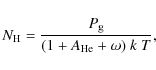
where k is the Boltzmann constant and T the temperature. The parameter to check the convergence of iterations is the electron-to-hydrogen ratio $\omega = (N_{\rm e}/N_{\rm H})$ . If $A_{\rm He}$ is the (He/H) abundance ratio, Eq. (4) becomes

$\begin{displaymath}P_{\rm g} = N_{\rm H} \left( 1 + A_{\rm He} + \omega \right)~k~T . \end{displaymath}$

(5)

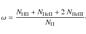
The model atom for hydrogen includes 5 discrete levels plus 1 continuum. The equations of radiative transfer for the 10 discrete transitions and the 5 bound-free transitions are treated in detail, except in the case where the optical thicknesses are very low, which generally happens for continua from subordinate levels. The model atom for helium is the same as in Labrosse & Gouttebroze (2001, 2004). It contains 34 levels: 29 for He I, 4 for He II, and 1 for He III. The main part of this model comes from the neutral helium model of Benjamin et al. (1999). It is complemented with parameters of various origins, as described in Labrosse and Gouttebroze (2001). The number of permitted radiative transitions is 76, but most of them are optically thin under the usual conditions. All discrete transitions, for hydrogen as for helium, are treated under the assumption of complete frequency redistribution.

Table 1: Summary of cylindrical thread models.

2.2 Computational scheme

The computation is organized along two parallel series of routines, one for hydrogen, the other for helium. In each series of routines, the variables dependent on the atomic structures as atomic parameters, populations, intensities in different transitions are gathered into a specific Fortran ``common'', which is ignored by the main program. This main program only contains geometric (D, r, $\psi$ , etc.) and physical ( $P_{\rm g}$ , T, v_T, etc.) variables and the populations ( $N_{\rm HII}$ , $N_{\rm HeII}$ , etc.) necessary to determine the ionization. The main phases of computations are:

initialization: determination of geometrical, physical and atomic parameters. The incident intensities are also computed for each position at the surface of the cylinder and each direction, according to the method explained in Paper II;
first evaluation of level populations, in the optically thin approximation. By averaging the incident intensities, we obtain mean intensities in the different transitions of hydrogen and helium. From these intensities and physical parameters, we compute the radiative and collisional transition rates. Then, we solve statistical equilibrium equations to obtain atomic level populations at each point of the ( $r,\psi$ ) mesh. Since the transition rates depend on electron density, it is necessary to iterate. We start from an arbitrary value of $\omega$ (e.g. $\omega=0.5$ ) and, using Eqs. (3) and (5), successively deduce:

$\begin{displaymath}N_{\rm H} = \frac{P_{\rm g}}{(1 + A_{\rm He} + \omega)~k~T}, \end{displaymath}$ (6)

$\begin{displaymath}N_{\rm He} = N_{\rm H} A_{\rm He}, \end{displaymath}$ (7)

and

$\begin{displaymath}N_{\rm e} = N_{\rm H}~\omega. \end{displaymath}$ (8)

After computation of transition rates and solution of statistical equilibrium equations, we compute $N_{\rm HII}$ , $N_{\rm HeII}$ , and $N_{\rm HeIII}$ by adding the populations of individual levels together, and deduce a new value of $\omega$ by

$\begin{displaymath}\omega = \frac {N_{\rm HII}+N_{\rm HeII}+2~ N_{\rm HeIII}} {N_{\rm H}}\cdot \end{displaymath}$ (9)

These operations are repeated until convergence.
full iterations with radiative transfer. This is the main part of the computation. The external scheme is similar to that of the preceding step, with a variable $\omega$ controlling the convergence of iterations but, in the meantime, the internal intensities for all transitions of hydrogen and helium are recomputed according to the principles of NLTE radiative transfer: absorption coefficients are derived from atomic level populations (determined in the preceding iteration). Then, intensities are computed by solving the transfer equation along each ray and integrating with respect to direction and frequency. At the same time, the diagonal terms of the $\Lambda$ operator are calculated by the method of Rybicki & Hummer (1991). The formulae appropriate to the cylindrical geometry are given in Paper II. The new intensities and the diagonal $\Lambda$ coefficients are used to form preconditioned statistical equilibrium equations, similar to those of Werner & Husfeld (1985). These equations are solved to obtain new level populations. Generally, one radiative transfer iteration for hydrogen and one for helium, between two iterations on $\omega$ , are sufficient to obtain a good convergence. In a few cases, it was necessary to perform two radiative transfer iterations for one $\omega$ iteration. These cases are indicated by an asterisk in the last column of Table 1.

2.3 Models

The model cylinders are defined by a series of geometric and physical parameters. The geometrical ones, diameter D, altitude Hand inclination $\alpha$ , have been defined above. Physical parameters include: gas pressure $P_{\rm g}$ , temperature T, microturbulent velocity v_T, and relative helium abundance $A_{\rm He}$ . The code allows the definition of each of these parameters as a function of r and $\psi$ , but this possibility is not used in practice, except for the temperature. A summary of models used in the present paper is displayed in Table 1. First, there is a series of isothermal models (``t1'' to ``t11'') with temperature ranging from 6000 to 10⁵ K. Their diameter is fixed to 1000 km, their pressure to 0.1 dyn cm^-2, helium abundance to 0.1, and microturbulent velocity to 5 km s^-1. Other models have a prescribed temperature variation T(r), which comes from Paper III, and is represented in the upper part of Fig. 1 (models using this temperature distribution are indicated by ``var.'' in the third column of Table 1). The mean model ``p4'' (or ``a4'') is similar to that of Paper III. In the series ``p1'' to ``p7'', we change the pressure while keeping the other parameters constant. In the series ``a1'' to ``a7'', we investigate the effects of helium abundance. The last column of Table 1 indicates the number of iterations necessary to achieve the convergence on $\omega$ , the criterion being fixed to 10^-6 and the minimum iteration number to 5.

3 Ionization

The introduction of helium ionization in models allows the electron density to be greater than the hydrogen density. Let $\xi=(N_{\rm HII}/N_{\rm H})$ be the ionization ratio for hydrogen, and similarly $\eta_1 = (N_{\rm HeII}/N_{\rm He})$ and $\eta_2 = (N_{\rm HeIII}/N_{\rm He})$ be the corresponding ratios for the two stages of helium ionization. Equation (9) becomes

$\begin{displaymath}\omega = \xi + A_{\rm He}~\eta_1 + 2~A_{\rm He}~\eta_2. \end{displaymath}$

(10)

The ionization ratios $\xi$ , $\eta _1$ and $\eta _2$ are principally controlled by temperature. However, near the surface of the structure, the influence of incident radiation becomes more important and tends to moderate the effects of temperature.

3.1 Model with temperature gradient

$\begin{figure} \par\includegraphics[width=9cm]{11483fg1.eps} \end{figure}$

Figure 1:

Variations of temperature T and population ratios with the distance to the axis (r), for the model ``p4'' at the foot of the loop ( $\alpha =0$ ). Abscissae: distance to axis relative to the total radius R. Top: temperature. Middle: ionization ratios for hydrogen ( $\xi$ : dot-dashed line) and helium ( $\eta _1$ : dashed line; $\eta _2$ : continuous line). Bottom: electron-to-hydrogen ratio $\omega$ (dashed line: model assuming neutral helium; continuous line: model with both hydrogen and helium ionization).

Open with DEXTER

In the standard model ``p4'', the temperature increases with the distance to the axis, as shown in the upper part of Fig. 1. In the core of the cylinder at 6000 K, helium is essentially neutral and hydrogen is weakly ionized, with a ratio $\xi$ between 0.2 and 0.3. The first ionization potential of hydrogen being lower than that of helium, $\xi$ begins to increase first when moving towards the exterior. This major change in hydrogen ionization occurs between 0.5 R and 0.7 R. For r > 0.7 R, which corresponds to temperatures T > 20 000 K, hydrogen is almost completely ionized. The first stage of ionization for helium (ratio $\eta _1$ ) occurs between (r/R)=0.7 and 0.8, i.e. temperatures between 20 000 and 35 000 K. The second stage of helium ionization starts near (r/R)=0.9, which corresponds to a temperature of 60 000 K. These variations of $\xi$ , $\eta _1$ and $\eta _2$ are represented in the middle part of Fig. 1. The consequences for electron density are shown in the lower part of Fig. 1, with a comparison to the case (Paper III) where helium ionization was neglected. The two curves practically coincide up to T=20 000 K, since hydrogen is the only electron contributor there. Between 30 000 and 60 000 K, $\omega$ remains close to 1.1, the main part of helium atoms being singly ionized. Near the surface, $\omega$ tends to 1.2, that is, the maximum possible value since we have assumed $A_{\rm He} = 0.1$ .

3.2 Isothermal models

$\begin{figure} \par\includegraphics[width=9cm]{11483fg2.eps} \end{figure}$

Figure 2:

Variations of the ionization ratios $\xi$ ( top) and $\eta _1$ ( bottom) with r for different isothermal models (for clarity, not all models are represented). Number densities are averaged with respect to the azimuth $\psi$ . Symbols for hydrogen: open circles: T = 6000 K; full circles: 8000 K; open squares: 10 000 K; full squares: 15 000 K; crosses: 20 000 K; continuous line: 50 000 K. Same symbols for helium, plus: dotted line: 30 000 K; dashed line: 65 000 K; dot-dashed line: 80 000 K.

Open with DEXTER

In the standard model, the variations of temperature with r masks the effects of incident radiation on ionization. To distinguish between thermal and radiative effects, it is necessary to examine the variations of ionization within isothermal models. We consider the series of ``t'' models described in Table 1. Here, the cylinders have horizontal axes, but the number densities are averaged over $\psi$ to obtain a single ionization curve ( $\xi(r)$ , $\eta_1(r)$ or $\eta_2(r)$ ) for each model and each ion species. Figure 2 represents the variations of ionization of hydrogen and helium for the different models of this series. It appears that the curves $\xi(r)$ and $\eta_1(r)$ are generally flat, which confirms that the effects of temperature dominate those of incident radiation. This is especially true for helium. For hydrogen, the $\xi(r)$ curves exhibit some inflexions near the surface. For the cool models at 6000 and 8000 K, the incident radiation tends to increase hydrogen ionization near the surface. In contrast, a decrease appears near the surface for models at 10 000 and 15 000 K. For temperatures higher than 20 000 K, the curves $\xi(r)$ are flat: hydrogen is almost completely ionized, so that the cylinders are optically thin in all transitions of the hydrogen atom, and consequently insensitive to incident radiation. Hydrogen is approximately half-ionized for T=10 000 K. The curves $\eta_1(r)$ corresponding to the first ionization stage of helium are very flat, but a slight decrease near the edge may be observed for the model at 20 000 K. The principal change of ionization for helium occurs between 20 000 K ( $\eta_1 \approx 0.3$ ) and 30 000 K ( $\eta_1 \approx 0.9$ ). Between 30 000 and 65 000 K, more than 90% of helium atoms are in the first stage of ionization (nearly 100% at 50 000 K). At higher temperatures, $\eta _1$ decreases while $\eta _2$ increases. At 80 000 K, the numbers of He II and He III ions are approximately equal. At 100 000 K, $\eta _1$ is lower than 0.2, and consequently $\eta _2$ greater than 0.8. The electron-to-hydrogen ratio $\omega$ (not represented) may be easily deduced from the curves of Fig. 2, according to Eq. (10). At low temperatures, $\omega$ is nearly equal to $\xi$ . In contrast, above 50 000 K, there are no longer neutral atoms, so that $\xi = 1$ and $\eta_2 = 1 - \eta_1$ , which gives $\omega \approx 1 + 0.1 \times ( 2 - \eta_1 )$ .

4 Formation of helium lines

The computations described in Sect. 2 provide us with absorption coefficients and source functions in the different lines of hydrogen and helium, which may be subsequently used to calculate the intensities emerging from the cylinder. The introduction of helium ionization has little influence on hydrogen lines, which are formed in regions where helium is essentially neutral. Since hydrogen lines have been treated in preceding papers, we concentrate here on helium lines, and use the standard model ``p4'' to study their formation.

$\begin{figure} \par\includegraphics[width=17cm]{11483fg3.eps} \end{figure}$	Figure 3: Emission of the loop model ``p4'' in several lines of helium: He I 10 830 Å ( top, left); He I 584 Å ( top, right); He I 5876 Å ( bottom, left); He II 304 Å ( bottom, right). Frequency-integrated intensities are normalized to the maximum value of each image. Horizontal and vertical coordinates indicate distances in megameters.
Open with DEXTER

The absorption coefficients and source functions for the different values of r and $\psi$ , are computed for 7 values of the inclination, from $\alpha =0$ to $\alpha=90\hbox{$^\circ$ }$ . Then, using an interpolation procedure described in Paper III, we construct a semi-toric loop model and obtain the intensities emitted towards the observer. Figure 3 shows the intensities, integrated over frequency, for a few lines chosen among the most important of the helium spectrum. The images corresponding to the two optical or infrared lines, say 10 830 and 5876 Å, look very similar to each other. The consideration of absorption coefficients indicates that the cylinder is optically thin for these two transitions (or marginally thick for 10 830 at line center). In contrast, the two ultraviolet lines, He I 584 and He II 304 Å, are definitely optically thick. The structure seems broader in He II than in He I lines, which is explained below.

$\begin{figure} \par\includegraphics[width=9cm]{11483fg4.eps} \end{figure}$	Figure 4: Ray path through the cylinder.
Open with DEXTER

$\begin{figure} \par\includegraphics[width=9cm]{11483fg5.eps} \end{figure}$	Figure 5: Total emergent intensities computed from model ``p4'', for different helium lines vs. position across the cylinder. Abscissae are in megameters and grow as the distance from the Sun. Ordinates are intensities in erg cm^-2 s^-1 sr^-1. Dashed line: He I 10 830 Å; dotted line: He I 5876 Å; dot-dashed line: He I 584 Å; continuous line: He II 304 Å.
Open with DEXTER

To discuss the process of formation, it is sufficient to consider the top of the loop, equivalent to a cylinder with a horizontal axis. For an observer looking at the cylinder in a direction normal to the axis, the path of photons is represented in Fig. 4. The ray enters the cylinder at point A and exits at point B. If R is the radius of the cylinder and $r_{\perp}$ the distance between the axis and the ray, the abscissae of A and B are $-s_{\rm max}$ and $s_{\rm max}$ , respectively, with

$\begin{displaymath}s_{\rm max} = \sqrt { R^2 - r_{\perp}^2 } . \end{displaymath}$

(11)

Let $\kappa_{\nu}$ and $S_{\nu}$ be the absorption coefficient and the source function, respectively, at frequency $\nu$ . From the transfer equation

$\begin{displaymath}\frac { {\rm d} I_{\nu} } { {\rm d} s } = \kappa_{\nu} ( S_{\nu} - I_{\nu} ), \end{displaymath}$

(12)

and the boundary condition

$\begin{displaymath}I_{\nu} ( - s_{\rm max} ) = 0, \end{displaymath}$

(13)

we deduce the emergent intensity

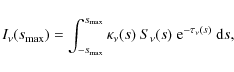$\begin{displaymath}I_{\nu} ( s_{\rm max} ) = \int_{-s_{\rm max}}^{s_{\rm max}} \kappa_{\nu}(s)~S_{\nu}(s)~{\rm e}^{-\tau_{\nu}(s)}~{\rm d}s, \end{displaymath}$

(14)

with the optical thickness between the running point M (abscissa s) and B

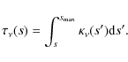$\begin{displaymath}\tau_{\nu} ( s ) = \int_{s}^{s_{\rm max}} \kappa_{\nu}(s') {\rm d}s'. \end{displaymath}$

(15)

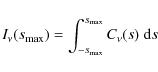
The total emergent intensity for the line under consideration is then

$\begin{displaymath}I_{\rm line} = \int_{\rm line} I_{\nu}(s_{\rm max})~{\rm d}\nu. \end{displaymath}$

(16)

These frequency-integrated intensities have been computed as functions of r and $\psi$ for different helium lines. They are shown in Fig. 5. For all these lines, we observe a global decrease of intensities from the lower to the upper edge, which is due to the decrease of incident radiation. However, several differences may be noticed. Concerning ultraviolet optically thick lines, the cylinder appears broader in the He II resonance line at 304 Å than in the corresponding line for He I at 584 Å. The two triplet lines of He I under consideration have in common a transversal variation with three smooth peaks.

To locate the origin of emission inside the cylinder, we rewrite Eq. (14) as

$\begin{displaymath}I_{\nu} ( s_{\rm max} ) = \int_{-s_{\rm max}}^{s_{\rm max}} C_{\nu}(s)~{\rm d}s \end{displaymath}$

(17)

with

$\begin{displaymath}C_{\nu}(s) = \kappa_{\nu}(s)~S_{\nu}(s)~{\rm e}^{-\tau_{\nu}(s)}. \end{displaymath}$

(18)

Thus, Eq. (16) becomes

$\begin{displaymath}I_{\rm line} = \int_{-s_{\rm max}}^{s_{\rm max}} C(s)~{\rm d}s \end{displaymath}$

(19)

with

$\begin{displaymath}C(s) = \int_{\rm line} C_{\nu}(s)~{\rm d}\nu. \end{displaymath}$

(20)

C(s) is the contribution function appropriate for the frequency-integrated emergent intensity. This function is plotted as shades of gray in Fig. 6 for the three lines at 10 830, 584 and 304 Å. The figure for the 5876 Å line is very similar to that of the 10 830 Å line. The existence of three maxima of emission for the intensity at 10 830 Å is due to the existence of two zones in the contribution function: a central patch and a ring. The patch corresponds to radiative processes of emission by low temperature matter, while the ring corresponds to a range of temperature where the maximum excitation of He I is occuring. The radiative processes of emission that occur in the central patch include direct scattering of incident radiation and the photoionization-recombination process (Hirayama 1971; Zirin 1975). Since these two processes are dependent on incident radiation, the contribution functions in the central zone decrease with height. In contrast, the ring is produced by collisional excitation, so that it is practically independent of $\psi$ . The contribution function for the 584 Å line is concentrated in a single ring, without a central part: since the line is optically thick, the front part of the ring only contributes to intensity. The same is true for the 304 Å line but, in this case, the emitting layer is located at high temperature, very close to the surface. For this reason, the loop looks broader in this transition than in the He I lines.

$\begin{figure} \par\includegraphics[width=6.7cm]{11483fg6.eps} \end{figure}$	Figure 6: Contribution functions corresponding to the standard model with a horizontal axis, for three lines of helium. Top: He I 10 830 Å; Middle: He I 584 Å; Bottom: He II 304 Å. Bright zones correspond to the maximum of the function. Directions are the same as in Fig. 4 (observer at right, Sun below).
Open with DEXTER

5 Influence of physical parameters

5.1 Temperature

$\begin{figure} \par\includegraphics[width=8.5cm]{11483fg7.eps} \end{figure}$	Figure 7: Frequency-integrated intensities, averaged over position, emitted by isothermal models ``t1'' to ``t11''. Intensities (erg cm^-2 s^-1 sr^-1) are plotted as functions of the temperature (K) of the model, in 4 transitions: He I 10 830 Å (open circles); He I 584 Å (full circles); He I 5876 Å (open squares); He II 304 Å (full squares).
Open with DEXTER

To study the effects of temperature on emitted intensities, we use the series of isothermal models ranging from ``t1'' (6000 K) to ``t11'' (10⁵ K). The cylinders under consideration have a horizontal axis ( $\alpha=90\hbox{$^\circ$ }$ ) and the emitted intensities are averaged along the transversal direction. This spatial averaging is convenient for comparison with most observations, where the width of the loops corresponds to a small number of pixels. Frequency-integrated intensities, for the different models and the four principal lines, are displayed in Fig. 7. The He I triplet lines at 10 830 and 5876 Å again show a similar behavior: the intensities decrease from 6000 to 15 000 K, rise from 15 000 to 30 000 K, and decrease again at higher temperatures. As mentioned in the preceding section, these lines have two sources of emission: radiative (dependent on incident radiation) and collisional. At low temperatures, scattering is dominant, and the decrease of optical thickness results in a decrease of scattered radiation. At higher temperatures, collisional excitation grows and, despite the decrease of optical thickness, the emitted intensity rises. For temperatures greater than 30 000 K, the effect of the opacity decrease (principally due to ionization, as may be seen in Fig. 2) dominates that of the excitation increase, so that the intensity decreases again. The intensity variation of the resonance line at 584 Å is similar, but this line is optically thick at low or medium temperatures, so that the slope of the curve between 6000 and 15 000 K is not as steep as that of the triplet lines. At high temperatures, the decrease of the 584 Å line intensity is faster than that of the triplet lines, which may be due to the decrease of density. According to the analysis of neutral helium line formation by Andretta and Jones (1997), the intensity ratio (triplet/singlet lines) decreases with increased density. The behavior of the resonance line of He II is quite different and shows a slow and steady increase of intensity with temperature until about 80 000 K, followed by a decrease. Most He II lines reach their peak of emission between $5\times10^4$ K and 10⁵ K (see for instance Laming and Feldman 1993 for the 1640 Å line).

$\begin{figure} \par\includegraphics[width=11.3cm,clip]{11483fg8.eps} \end{figure}$	Figure 8: Helium line half-profiles emitted by five isothermal models: continuous line: ``t1'' (6000 K); dashed line: ``t4'' (15 000 K); dotted line: ``t6'' (30 000 K); dot-dashed line: ``t8'' (50 000 K); long-dashed line: ``t11'' (100 000 K). Each frame corresponds to a specific line, as indicated.
Open with DEXTER

The consideration of line profiles (Fig. 8) gives another insight to the effects of temperature variations. The profiles of triplet lines are nearly Gaussian, a typical feature of optically thin lines, their widths increasing with temperature. The 584 Å line exhibits a reversed profile from 6000 to 30 000 K. At 50 000 K, the reversal disappears, indicating that the line is optically thin. This is due to the fast decrease of neutral helium populations above $3\times10^4$ K (see Fig. 2). At 10⁵ K, the central intensity of the 584 Å line is two orders of magnitude lower than at $5\times10^4$ K. For the He II line at 304 Å, the line center intensity is roughly constant until $5\times10^4$ K, and the global increase of intensity is due to the progressive broadening of the line profile. At these temperatures, the main process of emission is the scattering of incident radiation, and the broadening of the line is due to the joint effects of opacity (increase of $\eta _1$ ) and temperature (Doppler effect). Above $5\times10^4$ K, $\eta _1$ begins to decrease, but collisional excitation grows. These two competing effects produce a maximum of intensity near $8\times10^4$ K. In Fig. 8, one can compare the profiles of the 304 Å line at $5\times10^4$ and 10⁵ K: the higher temperature profile is more intense at line center, but the intensity decreases more rapidly in the wings, as a consequence of the lower opacity.

5.2 Pressure

The effects of gas pressure on emitted intensities are studied by means of a series of models ``p1'' to ``p7''. These models have the same variation of temperature as the standard model, but differ from each other by pressures ranging from 0.02 to 0.5 dyn cm^-2. Frequency-integrated intensities for the principal helium lines emitted by these models are displayed in Fig. 9. It appears that all intensities increase with pressure, but the slopes of the curves differ from one line to another. For neutral helium lines, the variation may be understood by considering the two main processes of emission: scattering of incident radiation and collisional excitation. In the optically thin case, the first process yields intensities proportional to atom populations. The second emission process, collisional excitation, which is proportional not only to the emitting atom density, but also to the electron density, tends to produce a quadratic variation of emission as a function of pressure. These considerations apply to the two He I lines at 10 830 and 5876 Å. It is visible in Fig. 9 that the emitted intensities for these two lines are proportional to pressure from 0.02 to about 0.2 dyn cm^-2, and that the slope slightly increases at higher pressures, when collisions cease to be negligible. The same considerations apply to the 584 Å line, but the change of slope begins at lower pressures, around 0.1 dyn cm^-2. The case of the He II 304 Å line is more complicated, since the slope of I(P) is less than linear below 0.1 dyn cm^-2 and greater than linear at higher pressures. It is visible on profiles (Fig. 8) that this line is optically thick and formed in the outermost part of the cylinder (Fig. 6). Whatever the pressure, the incident ultraviolet radiation from the Sun ionizes helium near the surface of the cylinder and creates a zone which scatters the 304 Å radiation. This part of emission due to scattering is nearly constant and constitutes the main contribution at low pressures (0.02 to 0.05 dyn cm^-2). In contrast, at high pressures (0.2 to 0.5 dyn cm^-2), collisional excitation becomes dominant and results in a quasi-quadratic variation of I(P).

$\begin{figure} \par\includegraphics[width=8.8cm]{11483fg9.eps} \end{figure}$	Figure 9: Frequency-integrated intensities, averaged over position, emitted by models ``p1'' to ``p7''. Abscissae: gas pressure inside the cylinder (dyn cm^-2). Ordinates: intensities in erg cm^-2 s^-1 sr^-1. Spectral lines: He I 10 830 Å (open circles); He I 584 Å (full circles); He I 5876 Å (open squares); He II 304 Å (full squares).
Open with DEXTER

5.3 Helium abundance

The abundance of helium is one of the most important parameters when analysing helium lines (see for instance Andretta et al. 2008, and references therein). Some observations, like that of filaments by Gilbert et al. (2007) suggest that very important changes of helium abundance may occur between the top, and the base of these objects. To evaluate the importance of this parameter to the emission of cylinder threads, we use a series of models (``a1'' to ``a7''), with the same pressure and temperature variation as the standard model, but helium to hydrogen ratios $A_{\rm He}$ varying from 0.01 to 0.3. The variations of intensities as functions of $A_{\rm He}$ are displayed in Fig. 10. The interpretation of these curves is relatively easy. As long as the cylinder is optically thin in the considered transition, the intensity is proportional to $A_{\rm He}$ . This is the case for the 10 830 and 5876 lines until $A_{\rm He}=0.05$ . For higher abundances, the slopes of the curves slightly decrease as the line centers begin to saturate. For optically thick lines at 584 and 304 Å, the intensity is still a growing function of abundance, but the slope is significantly lower than that corresponding to proportionality.

$\begin{figure} \par\includegraphics[width=9cm]{11483f10.eps} \end{figure}$	Figure 10: Frequency-integrated intensities, averaged over position, emitted by models ``a1'' to ``a7''. Abscissae: log (abundance ratio $A_{\rm He}$ ). Ordinates: intensities in erg cm^-2 s^-1 sr^-1. Spectral lines: He I 10 830 Å (open circles); He I 584 Å (full circles); He I 5876 Å (open squares); He II 304 Å (full squares).
Open with DEXTER

6 Conclusion

At this stage of our project, it is possible to perform a modeling of solar coronal loops including the following ingredients:

NLTE radiative transfer in cylindrical geometry;
2 dimensions (radius and azimuth);
statistical equilibrium of atomic level populations;
self-consistent treatment of the two principal chemical elements: hydrogen and helium, including ionization;
pressure equilibrium.

The numerical code produces in a single run spectral line profiles and intensities for the principal transitions of hydrogen and helium, emitted in all directions. Some developments remain to be done, such as the implementation of motions in helium routines (as was done for hydrogen in Paper V), or the treatment of Lyman lines in partial redistribution. We also are willing to apply our code to the modeling of complex loop systems observed in the solar atmosphere. We envisage to extend the code to some minor chemical species, as a function of the observed spectral lines.

Acknowledgements

We wish to thank Petr Heinzel for useful suggestions concerning this manuscript.

References

Andretta, V., & Jones, H. P. 1997, ApJ, 489, 375 [NASA ADS] [CrossRef] (In the text)
Andretta, V., Mauas, P. J. D., Falchi, A., & Teriaca, L. 2008, ApJ, 681, 650 [NASA ADS] [CrossRef] (In the text)
Benjamin, R. A., Skillman, E. D., & Smits, D. P. 1999, ApJ, 514, 307 [NASA ADS] [CrossRef] (In the text)
Gilbert, H. R., Kilper, G., & Alexander, D. 2007, ApJ, 671, 978 [NASA ADS] [CrossRef] (In the text)
Gouttebroze, P. 2004, A&A, 413, 733 [NASA ADS] [CrossRef] [EDP Sciences] (Paper I) (In the text)
Gouttebroze, P. 2005, A&A, 434, 1165 [NASA ADS] [CrossRef] [EDP Sciences] (Paper II) (In the text)
Gouttebroze, P. 2006, A&A, 448, 367 [NASA ADS] [CrossRef] [EDP Sciences] (Paper III) (In the text)
Gouttebroze, P. 2007, A&A, 465, 1041 [NASA ADS] [CrossRef] [EDP Sciences] (Paper IV) (In the text)
Gouttebroze, P. 2008, A&A, 487, 805 [NASA ADS] [CrossRef] [EDP Sciences] (Paper V) (In the text)
Heinzel, P. 2007, in The Physics of Chromospheric Plasmas, ed. P. Heinzel, I. Dorotovic, & R. J. Rutten, ASP Conf. Ser., 368, 271 (In the text)
Hirayama, T. 1971, Sol. Phys., 17, 50 [NASA ADS] [CrossRef] (In the text)
Labrosse, N., & Gouttebroze, P. 2001, A&A, 380, 323 [NASA ADS] [CrossRef] [EDP Sciences] (In the text)
Labrosse, N., & Gouttebroze, P. 2004, ApJ, 617, 614 [NASA ADS] [CrossRef] (In the text)
Laming, J. M., & Feldman, U. 1993, ApJ, 403, 434 [NASA ADS] [CrossRef] (In the text)
Patsourakos, S., Gouttebroze, P., & Vourlidas, A. 2007, ApJ, 664, 1214 [NASA ADS] [CrossRef] (In the text)
Rybicki, G. B., & Hummer, D. G. 1991, A&A, 245, 171 [NASA ADS] (In the text)
Werner, K., & Husfeld, D. 1985, A&A, 148, 417 [NASA ADS] (In the text)
Zirin, H. 1975, ApJ, 199, L63 [NASA ADS] [CrossRef] (In the text)

All Tables

Table 1: Summary of cylindrical thread models.

All Figures

$\begin{figure} \par\includegraphics[width=9cm]{11483fg1.eps} \end{figure}$	Figure 1: Variations of temperature T and population ratios with the distance to the axis (r), for the model ``p4'' at the foot of the loop ( $\alpha =0$ ). Abscissae: distance to axis relative to the total radius R. Top: temperature. Middle: ionization ratios for hydrogen ( $\xi$ : dot-dashed line) and helium ( $\eta _1$ : dashed line; $\eta _2$ : continuous line). Bottom: electron-to-hydrogen ratio $\omega$ (dashed line: model assuming neutral helium; continuous line: model with both hydrogen and helium ionization).
Open with DEXTER
In the text

$\begin{figure} \par\includegraphics[width=9cm]{11483fg2.eps} \end{figure}$	Figure 2: Variations of the ionization ratios $\xi$ ( top) and $\eta _1$ ( bottom) with r for different isothermal models (for clarity, not all models are represented). Number densities are averaged with respect to the azimuth $\psi$ . Symbols for hydrogen: open circles: T = 6000 K; full circles: 8000 K; open squares: 10 000 K; full squares: 15 000 K; crosses: 20 000 K; continuous line: 50 000 K. Same symbols for helium, plus: dotted line: 30 000 K; dashed line: 65 000 K; dot-dashed line: 80 000 K.
Open with DEXTER
In the text

$\begin{figure} \par\includegraphics[width=17cm]{11483fg3.eps} \end{figure}$	Figure 3: Emission of the loop model ``p4'' in several lines of helium: He I 10 830 Å ( top, left); He I 584 Å ( top, right); He I 5876 Å ( bottom, left); He II 304 Å ( bottom, right). Frequency-integrated intensities are normalized to the maximum value of each image. Horizontal and vertical coordinates indicate distances in megameters.
Open with DEXTER
In the text

$\begin{figure} \par\includegraphics[width=9cm]{11483fg4.eps} \end{figure}$	Figure 4: Ray path through the cylinder.
Open with DEXTER
In the text

$\begin{figure} \par\includegraphics[width=9cm]{11483fg5.eps} \end{figure}$	Figure 5: Total emergent intensities computed from model ``p4'', for different helium lines vs. position across the cylinder. Abscissae are in megameters and grow as the distance from the Sun. Ordinates are intensities in erg cm^-2 s^-1 sr^-1. Dashed line: He I 10 830 Å; dotted line: He I 5876 Å; dot-dashed line: He I 584 Å; continuous line: He II 304 Å.
Open with DEXTER
In the text

$\begin{figure} \par\includegraphics[width=6.7cm]{11483fg6.eps} \end{figure}$	Figure 6: Contribution functions corresponding to the standard model with a horizontal axis, for three lines of helium. Top: He I 10 830 Å; Middle: He I 584 Å; Bottom: He II 304 Å. Bright zones correspond to the maximum of the function. Directions are the same as in Fig. 4 (observer at right, Sun below).
Open with DEXTER
In the text

$\begin{figure} \par\includegraphics[width=8.5cm]{11483fg7.eps} \end{figure}$	Figure 7: Frequency-integrated intensities, averaged over position, emitted by isothermal models ``t1'' to ``t11''. Intensities (erg cm^-2 s^-1 sr^-1) are plotted as functions of the temperature (K) of the model, in 4 transitions: He I 10 830 Å (open circles); He I 584 Å (full circles); He I 5876 Å (open squares); He II 304 Å (full squares).
Open with DEXTER
In the text

$\begin{figure} \par\includegraphics[width=11.3cm,clip]{11483fg8.eps} \end{figure}$	Figure 8: Helium line half-profiles emitted by five isothermal models: continuous line: ``t1'' (6000 K); dashed line: ``t4'' (15 000 K); dotted line: ``t6'' (30 000 K); dot-dashed line: ``t8'' (50 000 K); long-dashed line: ``t11'' (100 000 K). Each frame corresponds to a specific line, as indicated.
Open with DEXTER
In the text

$\begin{figure} \par\includegraphics[width=8.8cm]{11483fg9.eps} \end{figure}$	Figure 9: Frequency-integrated intensities, averaged over position, emitted by models ``p1'' to ``p7''. Abscissae: gas pressure inside the cylinder (dyn cm^-2). Ordinates: intensities in erg cm^-2 s^-1 sr^-1. Spectral lines: He I 10 830 Å (open circles); He I 584 Å (full circles); He I 5876 Å (open squares); He II 304 Å (full squares).
Open with DEXTER
In the text

$\begin{figure} \par\includegraphics[width=9cm]{11483f10.eps} \end{figure}$	Figure 10: Frequency-integrated intensities, averaged over position, emitted by models ``a1'' to ``a7''. Abscissae: log (abundance ratio $A_{\rm He}$ ). Ordinates: intensities in erg cm^-2 s^-1 sr^-1. Spectral lines: He I 10 830 Å (open circles); He I 584 Å (full circles); He I 5876 Å (open squares); He II 304 Å (full squares).
Open with DEXTER
In the text

Current usage metrics show cumulative count of Article Views (full-text article views including HTML views, PDF and ePub downloads, according to the available data) and Abstracts Views on Vision4Press platform.

Data correspond to usage on the plateform after 2015. The current usage metrics is available 48-96 hours after online publication and is updated daily on week days.

Initial download of the metrics may take a while.