| Issue |
A&A
Volume 503, Number 3, September I 2009
|
|
|---|---|---|
| Page(s) | 1023 - 1036 | |
| Section | Catalogs and data | |
| DOI | https://doi.org/10.1051/0004-6361/200810798 | |
| Published online | 09 July 2009 | |
A variability sample catalogue selected from the Sydney Observatory Galactic Survey![[*]](/icons/foot_motif.png)
A. Fresneau1 - W. H. Osborn2
1 - Observatoire astronomique, UMR 7550, 11 rue de l'Université, 67000 Strasbourg,
France
2 -
Department of Physics, Central Michigan University, Mt. Pleasant, MI 48859, USA
Received 13 August 2008 / Accepted 1 July 2009
Abstract
Context. A set of
![]() stars brighter than about B-magnitude 14 and having at least three observations are identified in the Sydney Observatory Galactic Survey, carried out over the years 1892-1932 along the galactic equator section
stars brighter than about B-magnitude 14 and having at least three observations are identified in the Sydney Observatory Galactic Survey, carried out over the years 1892-1932 along the galactic equator section
![]() with galactic latitude
with galactic latitude
![]() .
Short-term (30 min) and long-term (decades) magnitude variations in the data set are analyzed.
.
Short-term (30 min) and long-term (decades) magnitude variations in the data set are analyzed.
Aims. Evidence is sought for a correlation between short-term and long-term variabilities which would identify stars in a non-quiescent phase.
Methods. We use a reduced proper motion diagram to classify the stars in our sample into probable dwarfs, giants and other types. The validity of the kinematical classification is checked using objective-prism spectroscopic classification for
![]() early-type stars. A search is made for statistical correlations between our variability indicators and physical and kinematical stellar properties.
early-type stars. A search is made for statistical correlations between our variability indicators and physical and kinematical stellar properties.
Results. We find that suspected photospheric activity for giant and dwarf stellar candidates is correlated with the time to cross the galactic thin disk. We estimate a significant apparent B-magnitude variation of ![]() 0.25 over the 40 years of photographic observations, and candidates for monitoring for possible photospheric activity at the present time are selected employing a statistical colour-diagram which uses the total proper motion component as a distance indicator.
0.25 over the 40 years of photographic observations, and candidates for monitoring for possible photospheric activity at the present time are selected employing a statistical colour-diagram which uses the total proper motion component as a distance indicator.
Conclusions. Follow up studies of our tentative findings are suggested. Toward this aim the derived data for the set of
![]() stars with variability information is archived as the variability Sample Catalogue. The data for a set of
stars with variability information is archived as the variability Sample Catalogue. The data for a set of
![]() stars along the section of the galactic equator
stars along the section of the galactic equator
![]() ,
,
![]() ,
and a set of of
,
and a set of of
![]() stars along the section of the galactic meridian
stars along the section of the galactic meridian
![]() ,
,
![]() is also archived as a quick-look facility for seeking long-term magnitude changes since the century-old photographic observations were obtained.
is also archived as a quick-look facility for seeking long-term magnitude changes since the century-old photographic observations were obtained.
Key words: surveys - stars: variables: general
1 General characteristics of the Sydney Observatory Galactic Survey
The Sydney Observatory Galactic Survey (SOGS) is a catalogue
of half a million stars down to about about B-magnitude ![]() in
two bands, one along the galactic equator
(
in
two bands, one along the galactic equator
(
![]() ,
,
![]() )
and the other along a galactic
meridian (
)
and the other along a galactic
meridian (
![]() ,
,
![]() ).
The catalogue has been created using the Sydney Observatory Astrographic
Program (SOAP) photographic plates, which were taken in the years
1892-1932 with a 33-cm aperture,
).
The catalogue has been created using the Sydney Observatory Astrographic
Program (SOAP) photographic plates, which were taken in the years
1892-1932 with a 33-cm aperture,
![]() astrographic refractor
of
astrographic refractor
of
![]() m focal length, to survey the declination zone from
m focal length, to survey the declination zone from
![]() to
to ![]() (an area of 2285 square degrees, or about
five percent of the sky).
The original sample of
(an area of 2285 square degrees, or about
five percent of the sky).
The original sample of
![]() stars
with J2000 equatorial coordinates and photographic (blue) magnitudes
mb at epoch
stars
with J2000 equatorial coordinates and photographic (blue) magnitudes
mb at epoch
![]() was compared to modern-epoch observations in the V-band
(the GSC 1.2) to produce the
was compared to modern-epoch observations in the V-band
(the GSC 1.2) to produce the
![]() stars
in SOGS. The catalog is available on line through the VizieR
system
stars
in SOGS. The catalog is available on line through the VizieR
system![]() with catalogue
identifications J/AJ/130/2701 for the section
along the galactic equator and J/A+A/469/1221 for the section along
the galactic meridian. Additional details about the SOGS are
given in Fresneau et al. (2005, 2007).
with catalogue
identifications J/AJ/130/2701 for the section
along the galactic equator and J/A+A/469/1221 for the section along
the galactic meridian. Additional details about the SOGS are
given in Fresneau et al. (2005, 2007).
The SOAP observing program consisted of 1400 overlapping fields of
![]() field-of-view centered on even and odd
degrees of declination (at B1900.0) and spaced proportionally in RA
by a quantity
field-of-view centered on even and odd
degrees of declination (at B1900.0) and spaced proportionally in RA
by a quantity
![]() .
The nominal B1900 coordinates of the
plate centers
.
The nominal B1900 coordinates of the
plate centers ![]() ,
(
,
(
![]() are given in Table 1 along with the numbers of regions (n),
the RA spacing (
are given in Table 1 along with the numbers of regions (n),
the RA spacing (
![]() )
of plate j, where
)
of plate j, where ![]() .
The mean epoch (and dispersion) of the observations for each zone is indicated.
The numbers (k,m) of fields sampled along the galactic meridian (
.
The mean epoch (and dispersion) of the observations for each zone is indicated.
The numbers (k,m) of fields sampled along the galactic meridian (![]() )
and
along the equator (
)
and
along the equator (![]() )
in each declination zone using the deeper
plates in constructing the SOGS are indicated. Blue-sensitive plates were employed (which have roughly a 1400 Å-wide bandwith around the Fraunhofer G-line at 4308 Å)
and no filter was used in the observations.
The photometric wide band system of the survey is noted b, close to the B
Johnson system (centered on
)
in each declination zone using the deeper
plates in constructing the SOGS are indicated. Blue-sensitive plates were employed (which have roughly a 1400 Å-wide bandwith around the Fraunhofer G-line at 4308 Å)
and no filter was used in the observations.
The photometric wide band system of the survey is noted b, close to the B
Johnson system (centered on
![]() Å).
The stellar magnitudes mb are derived from
the image diameters and a calibration curve (between image diameters and B-magnitude) computed for the Tycho 2 stars (Hog et al. 2000) detected on each plate.
Å).
The stellar magnitudes mb are derived from
the image diameters and a calibration curve (between image diameters and B-magnitude) computed for the Tycho 2 stars (Hog et al. 2000) detected on each plate.
Table 1:
Distribution of the B1900.0 centers of the 1400
![]() fields of the Sydney Observatory Astrographic Program.
fields of the Sydney Observatory Astrographic Program.
Exposures of 8 min were obtained of all 1400 fields, and the measures of the stars brigher than b-mag. 12 on these plates were used in the construction of the astrographic catalog (Urban et al. 1998). Less well known is that there were also systematic sets of longer exposure plates:
- a.
- the 740 fields centered on even-degree declinations were covered
by plates having three consecutive exposures of 30 min. The 30-min
plates have mean epochs 1915 or later and a limiting b-magnitude of
14.5 and were were intended to permit
star images to be separated from plate defects;
- b.
- the 660 fields
centered on odd-degree declinations were photographed
with a single exposure of 80 min. These plates have epochs earlier
than 1915 and the increased exposure time gave a
limiting b-magnitude of about 16;
- c.
- some very long exposure plates (3-6 h) were taken by
the SOAP observers to be used to make prints of objects of special
interest (Russell 1891); these have a b-magnitude limit
down to 18 as determined from a set of ten plates of the LMC
(Fresneau et al. 2005).
In the present study we examine the SOGS photometric data.
Because of the overlapping-field approach, taken together the
deeper SOAP plates contain three to four separate exposures
for each
![]() quarter of a standard field,
except of course along the 1
quarter of a standard field,
except of course along the 1![]() border of the survey zone.
Thus, SOGS data contain two distinct potential indicators of
variability. First, one can look at the differences in
the mb magnitudes derived from each of the three
30-min exposures on the same plate. The rms scatter
border of the survey zone.
Thus, SOGS data contain two distinct potential indicators of
variability. First, one can look at the differences in
the mb magnitudes derived from each of the three
30-min exposures on the same plate. The rms scatter
![]() generally can be taken as the internal photometric
error for the plate, which we will show is about
generally can be taken as the internal photometric
error for the plate, which we will show is about
![]() mag identical
to the internal error of similar photographic observations
(Ortiz-Gil et al. 1998; Lamareille et al. 2003).
Larger scatter may indicate rapid blue-light variability,
which we will call flickering. Similarly, there is the rms
scatter
mag identical
to the internal error of similar photographic observations
(Ortiz-Gil et al. 1998; Lamareille et al. 2003).
Larger scatter may indicate rapid blue-light variability,
which we will call flickering. Similarly, there is the rms
scatter ![]() of the measured mb magnitude for a
given star on different plates, both the 80-min and
30-min ones, during the 1892-1932 period of observation.
Large
of the measured mb magnitude for a
given star on different plates, both the 80-min and
30-min ones, during the 1892-1932 period of observation.
Large ![]() values may indicate long-term variability.
The data should therefore allow us to identify suspected
short-term variables (objects showing variations over the
three 30-min consecutive exposures) as well as possible
long-term variables (those exhibiting changes over the 40 years
needed to complete the SOAP) as long as
the variations are sufficiently large.
values may indicate long-term variability.
The data should therefore allow us to identify suspected
short-term variables (objects showing variations over the
three 30-min consecutive exposures) as well as possible
long-term variables (those exhibiting changes over the 40 years
needed to complete the SOAP) as long as
the variations are sufficiently large.
We must emphasize that the main use of the SOGS data is for statistical studies. While the lists of suspected variables can be expected to contain some physically interesting objects, they will also no doubt contain some spurious cases of variability. Individual objects should mainly be considered targets for follow-up studies, which could easily be done using the numerous wide-field multi-colour surveys now available on-line (Sesar et al. 2007) in order to gather additional information on the targets we selected with rudimentary data. Our main goal will be to investigate if there is any statistical correlation in our star sample between flickering and/or long-term variability and distance above the galactic plane. Such an effect is suggested by the observed changes in frequency of magnetically active stars with height above the galactic plane (West et al. 2006, 2008). We would like to connect, in the SOGS data, the stellar chromospheric activity in the optical with the orientation of the velocity ellipse of stellar systems that we determined as a function of the altitude over the galactic plane (Fresneau et al. 2007). Such a correlation might indicate a star's passage through the dense ISM of the thin disk has an effect on stellar chromospheric activity (seen in the optical), but other causes of chromospheric activity are perhaps more likely (e.g. magnetic effects) and no definitive conclusion about the source of such a correlation would be possible in view of the low accuracy of our data. Without a theory that could explain the observed variability with the dust scale height (Marshall el al. 2006), we suggest a linkage between the dust density distribution and the stellar distribution. We try to classify the SOGS sources into two physical categories of H-burning and He-burning candidates as a first step and to select, from the fully automated classification, a manageable list of targets suitable to learn more about the causes for variability. The chromospheric activity has been studied (West et al. 2008) and significant dispersion in the chromospheric activity-age relation is found even among coeval stars (Pace & Pasquini 2004). Our goal is to disentangle a category of stars linked to the thin disk crossing time.
2 Photometric performance in the SOGS
Our original sample contained
![]() measurements on
a set of 628 photographic plates taken in the years 1892-1932.
The photometric measurements were reduced to mb magnitudes
using Tycho-2 reference stars (Hog et al. 2000). The internal error of magnitudes
determined from a given plate has been estimated from
measurements on
a set of 628 photographic plates taken in the years 1892-1932.
The photometric measurements were reduced to mb magnitudes
using Tycho-2 reference stars (Hog et al. 2000). The internal error of magnitudes
determined from a given plate has been estimated from ![]() ,
the scatters of the measures for the various stars around
the mean values mb of the multiple exposures on the plate.
,
the scatters of the measures for the various stars around
the mean values mb of the multiple exposures on the plate.
![\begin{figure}
\par\includegraphics[width=9cm,clip]{10798f1.ps}
\end{figure}](/articles/aa/full_html/2009/33/aa10798-08/img44.png) |
Figure 1: The mean error in measured magnitude as a function of apparent magnitude mb. |
| Open with DEXTER | |
The plate-to-plate uncertainties, which we call the external error,
has been determined from the magnitudes measured for the same star
on different plates, either the pre-1915 80-min plates or
the post-1915 30-min triple exposure plates. Figure 1 shows
the internal error and the external errors for the 80-min and
30-min plates as a function of apparent magnitude mb.
The internal errors were derived from the full set of
![]() measurements. Two sets of the external (plate-to-plate) errors are shown in Fig. 1, one based on comparisons of magnitudes from
the single 80-min exposure plates (taken before
1915) and the second from comparisons of magnitudes
from the triple 30-min exposure plates (taken later
than 1915). The data from the triple-exposure plates have been put in 0.1 mag
bins and then averaged. Based on the graph, we adopt
(
measurements. Two sets of the external (plate-to-plate) errors are shown in Fig. 1, one based on comparisons of magnitudes from
the single 80-min exposure plates (taken before
1915) and the second from comparisons of magnitudes
from the triple 30-min exposure plates (taken later
than 1915). The data from the triple-exposure plates have been put in 0.1 mag
bins and then averaged. Based on the graph, we adopt
(
![]() )
mag as the typical error for a magnitude determined
from these century-old plates for stars fainter than apparent magnitude
mb=10 (which are about 95% from the sample of
)
mag as the typical error for a magnitude determined
from these century-old plates for stars fainter than apparent magnitude
mb=10 (which are about 95% from the sample of
![]() stars). We note that the external error for the
triple-exposure plates becomes larger for stars with
stars). We note that the external error for the
triple-exposure plates becomes larger for stars with
![]() ,
as was found previously for similar plates
(Dick et al. 1993; Geffert et al. 1996).
For all plates both the internal and
external errors increase for the brighter stars, reaching 0.6 for
mb=8. Our tentative explanation is that such large errors
result from the stellar images used in the brighter magnitude
determinations being overexposed.
,
as was found previously for similar plates
(Dick et al. 1993; Geffert et al. 1996).
For all plates both the internal and
external errors increase for the brighter stars, reaching 0.6 for
mb=8. Our tentative explanation is that such large errors
result from the stellar images used in the brighter magnitude
determinations being overexposed.
![\begin{figure}
\par\includegraphics[width=9cm,clip]{10798f2.ps}
\end{figure}](/articles/aa/full_html/2009/33/aa10798-08/img46.png) |
Figure 2: The cumulative frequency of the magnitude errors is plotted for observations performed after and before 1915. |
| Open with DEXTER | |
In order to identify genuine stellar outbursts in the set of
![]() observations over the period 1892-1932, we plot in Fig. 2 the cumulative distribution of the apparent magnitude mb internal error (derived from multiple exposure plates taken
before and after 1915) and the external error (derived from plate-to-plate). The curves indicate the probability (between 0 and 1 along the Y-axis) for a star to be observed with a scatter larger than the value
observations over the period 1892-1932, we plot in Fig. 2 the cumulative distribution of the apparent magnitude mb internal error (derived from multiple exposure plates taken
before and after 1915) and the external error (derived from plate-to-plate). The curves indicate the probability (between 0 and 1 along the Y-axis) for a star to be observed with a scatter larger than the value
![]() along the X-axis. The mean magnitude internal error is estimated to 0.25 after 1915 and 0.35 before 1915, suggesting an improvement in the photographic plate emulsion over the years. A difference in plate quality
is duly observed over the 40 years needed to complete the survey. We also observe in Fig. 2 that the mean external error is larger than the internal errors, on the order of 0.4, suggesting that a level of systematic effect around 0.3 mag has crept into the external calibration of the magnitude mb. The main result of these photometric accuracies is to suspect that a short-term variability observed at the level of 1 mag concerns less than 10% of the stellar sample and can be a signature of a particular photospheric activity.
along the X-axis. The mean magnitude internal error is estimated to 0.25 after 1915 and 0.35 before 1915, suggesting an improvement in the photographic plate emulsion over the years. A difference in plate quality
is duly observed over the 40 years needed to complete the survey. We also observe in Fig. 2 that the mean external error is larger than the internal errors, on the order of 0.4, suggesting that a level of systematic effect around 0.3 mag has crept into the external calibration of the magnitude mb. The main result of these photometric accuracies is to suspect that a short-term variability observed at the level of 1 mag concerns less than 10% of the stellar sample and can be a signature of a particular photospheric activity.
In order to add more information to the set of
![]() measurements of equatorial coordinates and apparent magnitude mb, the plates taken in period 1892-1932 have been compared to the GSC version 1.2. The GSC is derived from the Quick V survey (Lasker et al. 1990) V-bandpass plates made around 1980.
We obtain in this procedure proper motions (p.m.) and colour indices (mb-V).
The derived values are sufficient for our purposes so we have not made comparisons between the SOAP and other catalogs, such as the GSC II (Lasker et al. 2008) or 2MASS (Kleinmann 1992; Skrutskie et al. 2006).
The proper motions
measurements of equatorial coordinates and apparent magnitude mb, the plates taken in period 1892-1932 have been compared to the GSC version 1.2. The GSC is derived from the Quick V survey (Lasker et al. 1990) V-bandpass plates made around 1980.
We obtain in this procedure proper motions (p.m.) and colour indices (mb-V).
The derived values are sufficient for our purposes so we have not made comparisons between the SOAP and other catalogs, such as the GSC II (Lasker et al. 2008) or 2MASS (Kleinmann 1992; Skrutskie et al. 2006).
The proper motions ![]() are used to segregate the nearer stars from distant ones,
which we will refer to as foreground and background stars, respectively. We adopted
are used to segregate the nearer stars from distant ones,
which we will refer to as foreground and background stars, respectively. We adopted
![]() yr-1 as our threshold based on our estimate that the error in our proper motions is about 0.003'' yr-1, which follows from the
yr-1 as our threshold based on our estimate that the error in our proper motions is about 0.003'' yr-1, which follows from the ![]() 90-yr epoch difference between the SOAP and the Quick V survey and equatorial coordinates accurate at a 0.3'' level. We investigated the p.m. errors as function of the apparent magnitude mb and we observed that the level of 0.003'' yr-1 is similar to the result obtained in other studies dealing with the same type of 100-yr old observations (Ducourant et al. 2006).
90-yr epoch difference between the SOAP and the Quick V survey and equatorial coordinates accurate at a 0.3'' level. We investigated the p.m. errors as function of the apparent magnitude mb and we observed that the level of 0.003'' yr-1 is similar to the result obtained in other studies dealing with the same type of 100-yr old observations (Ducourant et al. 2006).
![\begin{figure}
\par\includegraphics[width=9cm,clip]{10798f3.ps}
\end{figure}](/articles/aa/full_html/2009/33/aa10798-08/img51.png) |
Figure 3:
The numbers N of foreground and background stars as function of the apparent magnitude
|
| Open with DEXTER | |
We plot in Fig. 3 the numbers N of foreground and background
stars as a function of apparent magnitude
![]() .
With the trends of
.
With the trends of
![]() for the foreground star numbers and
for the foreground star numbers and
![]() for the
background star numbers, we derive that the original sample of
for the
background star numbers, we derive that the original sample of
![]() stars is complete to magnitude
stars is complete to magnitude
![]() .
This follows from
computing the integral
.
This follows from
computing the integral
![]() dmb
that should be equal to the total observed number of
dmb
that should be equal to the total observed number of
![]() stars.
stars.
3 Calibration of a basic 2-D relation valid for stellar groups
The reduced proper motion (RPM) is defined as
![]() ,
where
,
where ![]() is the observed total p.m.
component (Luyten 1922; Hertzsprung 1929).
In our case, we only consider our derived p.m. significant,
and hence suitable for calculation of RPM, when
is the observed total p.m.
component (Luyten 1922; Hertzsprung 1929).
In our case, we only consider our derived p.m. significant,
and hence suitable for calculation of RPM, when
![]() yr-1. Using that
yr-1. Using that
![]() and
and
![]() (where T is the
transverse velocity in km s-1, d is the
distance in pc and Mb is the absolute b-magnitude),
then the RPM is
(where T is the
transverse velocity in km s-1, d is the
distance in pc and Mb is the absolute b-magnitude),
then the RPM is
![]() (we ignore the
total interstellar absorption Ab).
(we ignore the
total interstellar absorption Ab).
![\begin{figure}
\par\includegraphics[width=9cm,clip]{10798f4.ps}
\end{figure}](/articles/aa/full_html/2009/33/aa10798-08/img60.png) |
Figure 4:
Number N of stars with
|
| Open with DEXTER | |
Figure 4 shows the numbers N of SOGS stars with
![]() as a function of the quantity Hb. The trend shows a linear component
as a function of the quantity Hb. The trend shows a linear component
![]() ,
i.e. a power law
relation, suggesting that to Hb =14 we have a distance-limited sample with a constant transverse velocity. This indicates a distance-limited sample
(i.e., an absolute limiting magnitude
,
i.e. a power law
relation, suggesting that to Hb =14 we have a distance-limited sample with a constant transverse velocity. This indicates a distance-limited sample
(i.e., an absolute limiting magnitude
![]() )
for a stellar system with a constant transverse
velocity
)
for a stellar system with a constant transverse
velocity
![]() km s-1 and an apparent
magnitude
km s-1 and an apparent
magnitude
![]() ,
that we associate
with the Main Sequence stars in the solar neighborhoud,
and two bumps in the trend around
,
that we associate
with the Main Sequence stars in the solar neighborhoud,
and two bumps in the trend around
![]() and
and
![]() that we attribute to contamination
of the Main Sequence star system by other types of
stellar systems (probably giants).
This stellar sample can be associated
with the system of main sequence stars with
apparent magnitudes
that we attribute to contamination
of the Main Sequence star system by other types of
stellar systems (probably giants).
This stellar sample can be associated
with the system of main sequence stars with
apparent magnitudes
![]() that are predominant in
the solar neighborhood (Herbst & Sawyer 1981). The deviations from linearity at
that are predominant in
the solar neighborhood (Herbst & Sawyer 1981). The deviations from linearity at
![]() ,
equivalent to
,
equivalent to
![]() ,
and at
,
and at
![]() ,
equivalent to
,
equivalent to
![]() ,
suggests contamination of the Main Sequence sample at these values
by stars of different kinematical properties, likely giants.
The figure illustrates the usefulness of computing RPM since it
is equivalent to an absolute magnitude Mb with an
offset of
,
suggests contamination of the Main Sequence sample at these values
by stars of different kinematical properties, likely giants.
The figure illustrates the usefulness of computing RPM since it
is equivalent to an absolute magnitude Mb with an
offset of
![]() .
.
![\begin{figure}
\par\includegraphics[width=9cm,clip]{10798f5.ps}
\end{figure}](/articles/aa/full_html/2009/33/aa10798-08/img73.png) |
Figure 5: The relation between absolute magnitudes from objective prism spectra (MB) and the RPM quantity Hb for a set of 104 stars in SOGS. |
| Open with DEXTER | |
We want to derive from our observations of mb and ![]() some physical characteristic related to absolute magnitude in
order to derive a distance. We use a set of about 104 mostly
OB stars for which MK and HD spectral types have been determined
by objective-prism observations (Andersen 1977). Figure 5
compares the computed Hb with the absolute magnitude
MB derived from the spectral type and
corresponding tables (Strand 1963).
We note that objective-prism spectral classification for hot stars is not very efficient in
discriminating luminosity effects for hot stars
(Johnson & Morgan 1953). We find a linear trend
MB =0.86 H b-3.6 that has a correlation
coefficient of 0.93. We also show in Fig. 5 the lines
corresponding to
some physical characteristic related to absolute magnitude in
order to derive a distance. We use a set of about 104 mostly
OB stars for which MK and HD spectral types have been determined
by objective-prism observations (Andersen 1977). Figure 5
compares the computed Hb with the absolute magnitude
MB derived from the spectral type and
corresponding tables (Strand 1963).
We note that objective-prism spectral classification for hot stars is not very efficient in
discriminating luminosity effects for hot stars
(Johnson & Morgan 1953). We find a linear trend
MB =0.86 H b-3.6 that has a correlation
coefficient of 0.93. We also show in Fig. 5 the lines
corresponding to
![]() when T=50 km s-1 (upper line)
and T=20 km s-1 (lower line), which indicates the relationship is for
reasonable values of T. We adopt Mb =0.86 Hb-3.6, assuming the deviation from a 1:1 relation is an artifact of interstellar absorption Ab or uncalibrated effects in the relationship between Hb and MB.
when T=50 km s-1 (upper line)
and T=20 km s-1 (lower line), which indicates the relationship is for
reasonable values of T. We adopt Mb =0.86 Hb-3.6, assuming the deviation from a 1:1 relation is an artifact of interstellar absorption Ab or uncalibrated effects in the relationship between Hb and MB.
The scatter of about 1 mag in the upper part of the diagram
(![]() )
suggests this is the level of uncertainty
for absolute magnitudes, determined in this way, at least for O-A
stars. We observe that the absolute magnitudes derived from
our kinematical classification (by converting Hb into
MB) have similar precision to those from automated
classification of medium dispersion objective-prism observations
(von Hippel et al. 1994). We therefore conclude that, with a 1 mag uncertainty,
a star's absolute magnitude Mb can be derived from the observed
quantity
)
suggests this is the level of uncertainty
for absolute magnitudes, determined in this way, at least for O-A
stars. We observe that the absolute magnitudes derived from
our kinematical classification (by converting Hb into
MB) have similar precision to those from automated
classification of medium dispersion objective-prism observations
(von Hippel et al. 1994). We therefore conclude that, with a 1 mag uncertainty,
a star's absolute magnitude Mb can be derived from the observed
quantity
![]() .
.
![\begin{figure}
\par\includegraphics[width=9cm,clip]{10798f6.ps}
\end{figure}](/articles/aa/full_html/2009/33/aa10798-08/img76.png) |
Figure 6: The absolute magnitude Mb derived from the calibration of Fig. 5, is plotted as function of the colour index (b-V). |
| Open with DEXTER | |
We present in Fig. 6 the RPMD for the set of stars plotted in Fig. 5 and with absolute magnitudes determined from Mb=0.86 Hb-3.6 and with the colour index (b-V). Also shown are the ridge-lines corresponding to main sequence stars, red giants of Pop. I (RG I) and Pop. II (RGII) and blue horizontal branch stars (Chiu 1980). The RPMD shows that once we have estimated Mb from Hb, we can then estimate (B-V)0 from (mb-V) and the appropriate ridge-line. For example, for the Main Sequence the adjustment of Mb to the ( MB,(B-V)0) of the ridge-line yields a linear relation (B-V)0 = 0.26+ 0.82(mb-V) for converting our (mb - V) color index into a dereddened (B-V)0 color. We have not derived relationships between (B-V)0 and (mb-V) for non-main sequence stars, but we suggest that even with our dereddened colors we can segregate giants from dwarfs based on number counting, as shown in Fig. 4.
In summary, the advantage of a RPMD with calibrated
colour-magnitude relationships (Jones 1972) is that we can
obtain from our observed quantities (
![]() )
for
a large number of stars some basic physical information, such as
luminosity and radius, that can be investigated for a
correlation with variability. The traditional HR diagram (HRD)
in the (
)
for
a large number of stars some basic physical information, such as
luminosity and radius, that can be investigated for a
correlation with variability. The traditional HR diagram (HRD)
in the (
![]() )-plane for a magnitude-limited
sample (see, for example, Sowell et al. 2007) would obviously permit a more accurate separation
of H-burning and He-burning stars; such will be available
for our sample once the GAIA space-borne mission is completed around 2020 (Perrymann et al. 2000).
)-plane for a magnitude-limited
sample (see, for example, Sowell et al. 2007) would obviously permit a more accurate separation
of H-burning and He-burning stars; such will be available
for our sample once the GAIA space-borne mission is completed around 2020 (Perrymann et al. 2000).
4 Validity of the RPMD for stellar group classification in SOGS
We consider that the relationship derived in the previous section
is valid for the sample of stars in SOGS. We plot in Fig. 7
the numbers of foreground stars (those with
![]() yr-1)
and background stars (
yr-1)
and background stars (
![]() yr-1) as a function of
the (B-V)0 colour derived using our calibration
(B-V)0=0.26+0.82(mb-V). We note that Fresneau et al. (2007)
found no colour effect when deriving p.m. at the level of
0.002'' yr-1 by comparing century-old astrographic observations
and second-epoch Schmidt telescope ones used in the GSC 1.2 construction. While that
result was based on Tycho-2 stars (Hog et al. 2000) brighter than mb=12
(Fresneau et al. 2005), we presume it is valid for even fainter stars,
and hence no severe systematic effect has been introduced into
the data by our proper motion determinations.
yr-1) as a function of
the (B-V)0 colour derived using our calibration
(B-V)0=0.26+0.82(mb-V). We note that Fresneau et al. (2007)
found no colour effect when deriving p.m. at the level of
0.002'' yr-1 by comparing century-old astrographic observations
and second-epoch Schmidt telescope ones used in the GSC 1.2 construction. While that
result was based on Tycho-2 stars (Hog et al. 2000) brighter than mb=12
(Fresneau et al. 2005), we presume it is valid for even fainter stars,
and hence no severe systematic effect has been introduced into
the data by our proper motion determinations.
![\begin{figure}
\par\includegraphics[width=9cm,clip]{10798f7.ps}
\end{figure}](/articles/aa/full_html/2009/33/aa10798-08/img79.png) |
Figure 7:
Numbers N of foreground (
|
| Open with DEXTER | |
We see in Fig. 7 that the numbers of foreground and
background stellar candidates are similar when the derived color
(B-V)0 is redder than 0.8 mag. We also notice that the
maximum number of foreground stars occurs a little redder
than the Parenago's discontinuity at
![]() .
The linear trends for
stars bluer than
(B-V)0=0.4 in the two systems suggest that most of
the background stars (those with unsignificant p.m.)
are hotter than the foreground stars and hence are
visible at distances larger than those that
produce a noticeable p.m.
We suggest therefore that our kinematical selection
criterion of
.
The linear trends for
stars bluer than
(B-V)0=0.4 in the two systems suggest that most of
the background stars (those with unsignificant p.m.)
are hotter than the foreground stars and hence are
visible at distances larger than those that
produce a noticeable p.m.
We suggest therefore that our kinematical selection
criterion of
![]() yr-1 yields
a stellar sample of mostly F-G stars, with distances out to
d=500 pc and a mixture of varying metallicities (Roman 1950; Ivezic et al. 2008).
Thus, the SOGS data provide a good source for extending
analyses of the local system of stars (Nordström et al. 2004). It is
known (Binney et al. 2000) that stars redwards to the Parenago's discontinuity
typically have a transverse velocity in the galactic plane
yr-1 yields
a stellar sample of mostly F-G stars, with distances out to
d=500 pc and a mixture of varying metallicities (Roman 1950; Ivezic et al. 2008).
Thus, the SOGS data provide a good source for extending
analyses of the local system of stars (Nordström et al. 2004). It is
known (Binney et al. 2000) that stars redwards to the Parenago's discontinuity
typically have a transverse velocity in the galactic plane
![]() km s-1 and stars bluewards a transverse velocity
km s-1 and stars bluewards a transverse velocity
![]() km s-1.
km s-1.
We can use the relation
Mb=-3.6+0.86 Hb to estimate a
distance modulus
![]() ,
and can use the
derived distance d to compute the star's altitude z
above the galactic plane
,
and can use the
derived distance d to compute the star's altitude z
above the galactic plane
![]() in the galactic latitude
direction b. We then use the Parenago's discontinuity to
check if we are really separating distinct stellar groups.
Figure 8 plots the numbers N of stars
(
in the galactic latitude
direction b. We then use the Parenago's discontinuity to
check if we are really separating distinct stellar groups.
Figure 8 plots the numbers N of stars
(
![]() )
bluer and redder than
(B-V)0=0.62, the Parenago discontinuity value,
as function of computed altitude over the galactic plane
z in pc. We expect stars bluer than
(B-V)0=0.62
to have lifetimes smaller than the age of the Galaxy
and to more likely be members of the thin disk and
those redder to have a higher probability
of belonging to the thick disk, the two
populations having significantly different scale heights
of about 300 and 900 pc respectively
(Bahcall & Soneira 1980; Gilmore & Reid 1983; Juric et al. 2008; Siegel et al. 2002; Bensby et al. 2004).
The thin disk stellar candidates belong to
a much flatter system, with a scale height on the
order of 250-300 pc. The results show the bluer stars are indeed
more concentrated to the galactic plane than the redder
ones. With our low accuracy data, we cannot claim
to segregate the stellar populations as well
as can be done with the extensive data from modern surveys (Munn et al. 2004).
)
bluer and redder than
(B-V)0=0.62, the Parenago discontinuity value,
as function of computed altitude over the galactic plane
z in pc. We expect stars bluer than
(B-V)0=0.62
to have lifetimes smaller than the age of the Galaxy
and to more likely be members of the thin disk and
those redder to have a higher probability
of belonging to the thick disk, the two
populations having significantly different scale heights
of about 300 and 900 pc respectively
(Bahcall & Soneira 1980; Gilmore & Reid 1983; Juric et al. 2008; Siegel et al. 2002; Bensby et al. 2004).
The thin disk stellar candidates belong to
a much flatter system, with a scale height on the
order of 250-300 pc. The results show the bluer stars are indeed
more concentrated to the galactic plane than the redder
ones. With our low accuracy data, we cannot claim
to segregate the stellar populations as well
as can be done with the extensive data from modern surveys (Munn et al. 2004).
![\begin{figure}
\par\includegraphics[width=9cm,clip]{10798f8.ps}
\end{figure}](/articles/aa/full_html/2009/33/aa10798-08/img85.png) |
Figure 8:
Numbers N of stars (
|
| Open with DEXTER | |
We point out that we assumed
![]() ,
but
given the low accuracy of our magnitudes
(
,
but
given the low accuracy of our magnitudes
(
![]() mag) a more accurate
approach is not warranted. Similarly, we felt it
was sufficient to merely apply the basic trigonometric
relations between distance and galactic coordinates
(l,b) and neglect such corrections as the effect
of the sun's galactic altitude
mag) a more accurate
approach is not warranted. Similarly, we felt it
was sufficient to merely apply the basic trigonometric
relations between distance and galactic coordinates
(l,b) and neglect such corrections as the effect
of the sun's galactic altitude
![]() pc
on the calculations (Bash 1986; Larsen & Humphreys 2003).
pc
on the calculations (Bash 1986; Larsen & Humphreys 2003).
To this point, we have mainly been counting numbers related to the observational data in SOGS (equatorial coordinates, p.m. components, mb and V magnitudes). This was done in an attempt to show how the data can be used to identify stellar groups with different scale heights that can be linked to an age effect using that the blue stars are younger. In the following sections of this paper, we investigate the information added by stellar variability data.
5 Construction of the variability sample catalog (VSC)
From the approximately
![]() stars in the SOGS
having p.m. sufficiently large that we can estimate a distance,
we extracted about
stars in the SOGS
having p.m. sufficiently large that we can estimate a distance,
we extracted about
![]() stars for which there
are at least one triple image plate and at least three separate
plates (which may include triple image plates) taken on diferent
dates over the 1892-1932 SOGS observation period. This comprises
a stellar sample suitable for investigating possible variability.
We call this stellar set the variability sample catalog (VSC).
stars for which there
are at least one triple image plate and at least three separate
plates (which may include triple image plates) taken on diferent
dates over the 1892-1932 SOGS observation period. This comprises
a stellar sample suitable for investigating possible variability.
We call this stellar set the variability sample catalog (VSC).
![\begin{figure}
\par\includegraphics[width=9cm,clip]{10798f9.ps}
\end{figure}](/articles/aa/full_html/2009/33/aa10798-08/img89.png) |
Figure 9: The reduced proper motion diagram (RPMD) [Hb,(b-V)] of the VSC stars that results by converting to a Mb, (B-V)0 diagram by applying the relations Mb=0.86 Hb-3.6 and (B-V)0=0.82(b-V)+0.26 as determined from Figs. 5 and 6. |
| Open with DEXTER | |
The reduced proper motion diagram (RPMD) for the stars in the
VSC, i.e. their positions in the
(Hb, mb-V)-plane
is shown in Fig. 9. Adopting the same ridge lines in the (
MB,[B-V]0)-plane as defined in Table 9 of Chiu (1980),
we estimated absolute magnitudes -
![]() - and dereddened colour -
- and dereddened colour -
![]() (Fresneau 1994). These relations follow
from the assumption that the mean dispersion of the transverse
velocity of foreground stars observed along the direction of each
(Fresneau 1994). These relations follow
from the assumption that the mean dispersion of the transverse
velocity of foreground stars observed along the direction of each
![]() field of view is on the order of 45 km s-1 (Fresneau et al. 2003).
These relations between Hb and Mb are based on a different stellar sample (Fresneau et al. 2005) than the one used in Sect. 4. The ridge-lines allow the derivation of an interstellar extinction
Ab that we estimate as approximately 1 mag kpc-1.
A
MB,(B-V)0 Main Sequence (MS I) is fitted in the
[Hb,(b-V)] plane of the Pop. I suggested stellar system
(without applying any bolometric corrections) to convert
the b-magnitude into the Johnson B photometric system.
field of view is on the order of 45 km s-1 (Fresneau et al. 2003).
These relations between Hb and Mb are based on a different stellar sample (Fresneau et al. 2005) than the one used in Sect. 4. The ridge-lines allow the derivation of an interstellar extinction
Ab that we estimate as approximately 1 mag kpc-1.
A
MB,(B-V)0 Main Sequence (MS I) is fitted in the
[Hb,(b-V)] plane of the Pop. I suggested stellar system
(without applying any bolometric corrections) to convert
the b-magnitude into the Johnson B photometric system.
One then finds a correlation
between the statistically derived parallax ![]() in 10-3 arcsec
and the p.m. total component
in 10-3 arcsec
and the p.m. total component ![]() in 10-3 arcsec yr-1 -
in 10-3 arcsec yr-1 -
![]() - which
is similar to the relation that was found using stars with
measured trigonometric parallax
- which
is similar to the relation that was found using stars with
measured trigonometric parallax
![]() arcsec
and p.m.
arcsec
and p.m.
![]() arcsec yr-1
in the space-based Hipparcos survey of stars brighter than apparent
magnitude 11 (Fresneau et al. 2005). We have not checked to
see if this result is changed by the recent improvements in the
Hipparcos catalog (van Leeuwen 2007; Perryman 2009).
arcsec yr-1
in the space-based Hipparcos survey of stars brighter than apparent
magnitude 11 (Fresneau et al. 2005). We have not checked to
see if this result is changed by the recent improvements in the
Hipparcos catalog (van Leeuwen 2007; Perryman 2009).
In our study, we will call the the 2-D diagram derived
from the RPMD, plotted as [Mb,(b-V)], as the
statistical HRD and call the parallax
![]() ,
derived from the d (in pc) given by the distance modulus
,
derived from the d (in pc) given by the distance modulus
![]() ,
as the statistical parallax.
,
as the statistical parallax.
Using
![]() and
and
![]() ,
we consider the [
(B-V)0,MB]
ridge-line that is closest to the star's position in the [(b-V),Hb]
RPMD to estimate MB. The set of coefficients
(
,
we consider the [
(B-V)0,MB]
ridge-line that is closest to the star's position in the [(b-V),Hb]
RPMD to estimate MB. The set of coefficients
(
![]() )
is derived from the
fit of the MS stars. Because we use p.m. as our distance indicator,
the error in p.m. can be converted to a standard deviation
in the statistical parallax that allows us to assess the
uncertainty of the absolute magnitude determinations.
We estimate this error from the variation in p.m. derived
from different plate pairs. The absolute
magnitude is
)
is derived from the
fit of the MS stars. Because we use p.m. as our distance indicator,
the error in p.m. can be converted to a standard deviation
in the statistical parallax that allows us to assess the
uncertainty of the absolute magnitude determinations.
We estimate this error from the variation in p.m. derived
from different plate pairs. The absolute
magnitude is
![]() ,
so the the error
,
so the the error
![]() resulting from a p.m. error
resulting from a p.m. error ![]() is
is
![]() .
Using
.
Using
![]() ,
we adopt
,
we adopt
![]() as the
reliability in M resulting from the error in p.m.
as the
reliability in M resulting from the error in p.m.
The data for the stars in the variability sample catalog (VSC)
is available on-line under anonymous
ftp![]() .
The catalog gives for each star the mean equatorial coordinates
(Equinox 2000), V-magnitude (taken from the GSC 1.2), mean
mb (from SOAP), mean dereddened colour index
(B-V)0 (obtained by comparing the star's location in the
(Hb, b-V) RPMD with the (
MB, [B-V]0) ridge-lines
defined by Table 9 of Chiu 1980), short-term apparent
magnitude scatter
.
The catalog gives for each star the mean equatorial coordinates
(Equinox 2000), V-magnitude (taken from the GSC 1.2), mean
mb (from SOAP), mean dereddened colour index
(B-V)0 (obtained by comparing the star's location in the
(Hb, b-V) RPMD with the (
MB, [B-V]0) ridge-lines
defined by Table 9 of Chiu 1980), short-term apparent
magnitude scatter ![]() ,
long-term apparent magnitude
scatter
,
long-term apparent magnitude
scatter ![]() ,
error in absolute magnitude determination
due to the p.m. component error
,
error in absolute magnitude determination
due to the p.m. component error
![]() ,
annual p.m. in arcsec
in galactic longitude
,
annual p.m. in arcsec
in galactic longitude ![]() and in galactic latitude
and in galactic latitude ![]() ,
derived parallax
,
derived parallax ![]() in milliarcsec, and a
correlation coefficient c, which has values from 0 to 1.0 and
will be explained later in our study. We also give our adopted
classification of the star as a Pop. I main sequence (MS I),
red giant (RG I), or white dwarf (WD I) or a Pop. II
subdwarf (SD II), red giant (RG II) or horizontal branch
(HB II) star based on the statistical HRD that results
from the observed blue (
in milliarcsec, and a
correlation coefficient c, which has values from 0 to 1.0 and
will be explained later in our study. We also give our adopted
classification of the star as a Pop. I main sequence (MS I),
red giant (RG I), or white dwarf (WD I) or a Pop. II
subdwarf (SD II), red giant (RG II) or horizontal branch
(HB II) star based on the statistical HRD that results
from the observed blue (![]() mb) and
V magnitudes and p.m. components as explained in our
previous studies (Fresneau 1990).
mb) and
V magnitudes and p.m. components as explained in our
previous studies (Fresneau 1990).
The kinematical information permits us to separate the star sample into H-burning or He-burning stellar candidates. We emphasize that, as for our variability criteria, this technique of stellar classification primarily allows one to identify a set of objects to be further investigated. Cuisinier et al. (1994) found they could identify halo dwarfs with a success rate of 10%. Smart et al. (2007) used a RPMD to identify extreme sub-dwarf candidates in the LHS Hipparcos-sample. These results show that a [Hb,b-V] RPMD cannot only be a substitute for the traditional HRD [ MB,(B-V)0] when parallax (hence absolute magnitude) is not available (Hertzsprung 1929), but also suggest that this is a straightforward way to explore a magnitude-limited stellar sample having only p.m. and apparent magnitudes in two passbands (Finch et al. 2007). This then makes it very attractive for extracting information from the extensive photographic surveys of the past (Luyten 1977; Gliese & Jahreiss 1980), even when work with century-old astrographic plate material generally relegated to history (Chinnici 2008) has an archaeological tinge. We recognize that modern CCD observations have significantly higher precision than photographic images from the past. However, our interest is in the possibility of using this largely neglected observational material on the most densely star-studded regions in the sky to harvest astrophysically interesting targets (for which there would be some baseline temporal information) for follow up by present day surveys (Munn et al. 2004; Kilic et al. 2006; Finch et al. 2007; Becker et al. 2004).
Figure 10 shows the statistical HRD for the VSC sample of
![]() stars using the values of (B-V)0 and
absolute magnitude Mb obtained from the RPMD.
Pop. I and Pop. II sequences (MS = main sequence, RG = red giants, HB = horizontal branch)
are easily visible and are labeled. The plot parameters are Mb=0.772 Hb-3.12 and
(B-V)0=0.84(mb-V)+0.38.
This figure illustrates how a statistical
HRD allows one to classify a star on the probability,
from its kinematical properties, that it is
a MS I, RG I, WD I, SD II, RG II or HB II star.
We emphasize, however, that our classification technique
based on ridge-lines
forces stars to belong either the Pop. I or Pop. II sequence,
without the possibility to fill any other locations in the diagram.
We also label in the figure what we tentatively suggest to be
an instability strip (I.S.) based on an excess of stars along
the vertical line of approximately constant color
stars using the values of (B-V)0 and
absolute magnitude Mb obtained from the RPMD.
Pop. I and Pop. II sequences (MS = main sequence, RG = red giants, HB = horizontal branch)
are easily visible and are labeled. The plot parameters are Mb=0.772 Hb-3.12 and
(B-V)0=0.84(mb-V)+0.38.
This figure illustrates how a statistical
HRD allows one to classify a star on the probability,
from its kinematical properties, that it is
a MS I, RG I, WD I, SD II, RG II or HB II star.
We emphasize, however, that our classification technique
based on ridge-lines
forces stars to belong either the Pop. I or Pop. II sequence,
without the possibility to fill any other locations in the diagram.
We also label in the figure what we tentatively suggest to be
an instability strip (I.S.) based on an excess of stars along
the vertical line of approximately constant color
![]() from Mb=1 to Mb=3
and down to the WD region. In the case of variability candidates,
the identification of an instability strip (I.S.) location
is probably a way to identify some potentially interesting targets
among misclassified stars.
A well-developed Red Giant
Branch (RG I) at
from Mb=1 to Mb=3
and down to the WD region. In the case of variability candidates,
the identification of an instability strip (I.S.) location
is probably a way to identify some potentially interesting targets
among misclassified stars.
A well-developed Red Giant
Branch (RG I) at
![]() and
and
![]() is identified redwards to the Hertzsprung gap.
Little else can be said without
additional observations on these targets other than there
appears to be some kind of feature in the diagram
(reflecting the I.S.) that extends from the HBII through
the MS I and down to the hot WD regime.
is identified redwards to the Hertzsprung gap.
Little else can be said without
additional observations on these targets other than there
appears to be some kind of feature in the diagram
(reflecting the I.S.) that extends from the HBII through
the MS I and down to the hot WD regime.
![\begin{figure}
\par\includegraphics[width=9cm,clip]{10798f10.ps}
\end{figure}](/articles/aa/full_html/2009/33/aa10798-08/img113.png) |
Figure 10:
The statistical HRD for the Variable Sample Catalogue
(VSC) set of
|
| Open with DEXTER | |
We again emphasize that Fig. 10 is just a convenient way
to roughly classify stars in a survey with rudimentary
information on colour and an RPM quantity.
Our classification is not exact
and does not yield pure Pop. I and Pop. II groups. For example,
in the
![]() stars of Fig. 10, our classification
gives
stars of Fig. 10, our classification
gives
![]() Pop. II candidates and
Pop. II candidates and
![]() Pop. I
candidates, which suggests poor classification efficiency since Pop. I
stars should outnumber the Pop. II stars by a factor of about
500 (Bahcall & Casertano 1986). A set of 80% of all observed stars
in a magnitude
Pop. I
candidates, which suggests poor classification efficiency since Pop. I
stars should outnumber the Pop. II stars by a factor of about
500 (Bahcall & Casertano 1986). A set of 80% of all observed stars
in a magnitude
![]() )
and distance (
)
and distance (
![]() )
limited sample should lie on the main sequence MS I, not just a set
of 60% as we observe (Allen 1973; Sowell et al. 2007). Nevertheless, the
data are adequate statistically to investigate how
stellar properties are correlated; this was demonstrated in a
previous study where stars classified as Pop. I candidates
were used to trace the thin disk kinematics in the solar
neighborhood up to a distance of 500 pc (Fresneau et al. 2005).
)
limited sample should lie on the main sequence MS I, not just a set
of 60% as we observe (Allen 1973; Sowell et al. 2007). Nevertheless, the
data are adequate statistically to investigate how
stellar properties are correlated; this was demonstrated in a
previous study where stars classified as Pop. I candidates
were used to trace the thin disk kinematics in the solar
neighborhood up to a distance of 500 pc (Fresneau et al. 2005).
6 Stellar variability information in the VSC
We use the VSC sample of
![]() stars from SOAP
that have magnitudes determined from at least three separate
plates and at least one set of three measures on the same
plate to look for statistical stellar variability effects.
We have, of course, to keep in mind the uncertainties
of
stars from SOAP
that have magnitudes determined from at least three separate
plates and at least one set of three measures on the same
plate to look for statistical stellar variability effects.
We have, of course, to keep in mind the uncertainties
of
![]() for our apparent magnitudes and 1.0 for the
estimated absolute magnitudes.
for our apparent magnitudes and 1.0 for the
estimated absolute magnitudes.
The two fundamental indicators of variability are the rms
magnitude scatter indices ![]() (called flickering)
and
(called flickering)
and ![]() (the long-term apparent magnitude scatter).
Because we want to associate the variability indicators
with particular types of stars, as classified in Fig. 10,
we also are interested in absolute magnitudes. Our derived
absolute magnitudes have uncertainties arising from two
sources: plate-to-plate differences in the measured
apparent magnitudes and errors in the distance determinations.
We therefore compute an additional scatter index
(the long-term apparent magnitude scatter).
Because we want to associate the variability indicators
with particular types of stars, as classified in Fig. 10,
we also are interested in absolute magnitudes. Our derived
absolute magnitudes have uncertainties arising from two
sources: plate-to-plate differences in the measured
apparent magnitudes and errors in the distance determinations.
We therefore compute an additional scatter index ![]() that results from the scatter in the p.m.
that results from the scatter in the p.m. ![]() .
The scatter
.
The scatter ![]() can be used to estimate the errors in the absolute
magnitude determinations that result from errors in the
distance calculations. Therefore, we adopt as our
measure for the uncertainty of a given absolute magnitude
Mb in the VSC
can be used to estimate the errors in the absolute
magnitude determinations that result from errors in the
distance calculations. Therefore, we adopt as our
measure for the uncertainty of a given absolute magnitude
Mb in the VSC
![]() .
A particularly large value of
.
A particularly large value of ![]() may reflect
either long-term variability
may reflect
either long-term variability ![]() or
an inaccurate distance determination.
or
an inaccurate distance determination.
![\begin{figure}
\par\includegraphics[width=9cm,clip]{10798f11.ps}
\end{figure}](/articles/aa/full_html/2009/33/aa10798-08/img118.png) |
Figure 11:
Short-term |
| Open with DEXTER | |
Figure 11 shows how the three variability
measures ![]() ,
,
![]() ,
,
![]() depend on
apparent magnitude mb. The
depend on
apparent magnitude mb. The
![]() points have been divided into 400 equally-spaced bins and each plotted point represents the rms of the
value in a bin. We rediscover (as from Fig. 1) that stars
brighter than mb=10 show the largest scatter, as
is expected since these stellar images will tend to be
overexposed. This indicates that the VSC sample should be
considered a survey of moderately faint stars, in the
apparent magnitude range
points have been divided into 400 equally-spaced bins and each plotted point represents the rms of the
value in a bin. We rediscover (as from Fig. 1) that stars
brighter than mb=10 show the largest scatter, as
is expected since these stellar images will tend to be
overexposed. This indicates that the VSC sample should be
considered a survey of moderately faint stars, in the
apparent magnitude range
![]() ,
for which
,
for which
![]() and
and
![]() .
We restrict the rest of our analysis to stars fainter than
mb=10 (97% of the VSC).
.
We restrict the rest of our analysis to stars fainter than
mb=10 (97% of the VSC).
Figures 12 and 13 show how the three variability
indicators ![]() ,
,
![]() ,
,
![]() depend on colour
(B-V)0 and on computed absolute magnitude MB for stars
with
depend on colour
(B-V)0 and on computed absolute magnitude MB for stars
with
![]() .
We see that:
.
We see that:
- a.
 ,
our measure of internal magnitude scatter
on one plate, ranges from about 0.8 for
,
our measure of internal magnitude scatter
on one plate, ranges from about 0.8 for
 to 0.5 for
 ;
;
- b.
 ,
the scatter in long-term variability
in apparent magnitude, which is our indicator of the random
plate-to-plate error, is systematically larger than
and fluctuates between 0.7 and 0.9;
,
the scatter in long-term variability
in apparent magnitude, which is our indicator of the random
plate-to-plate error, is systematically larger than
and fluctuates between 0.7 and 0.9;
- c.
 ,
the p.m. contribution to the absolute
magnitude uncertainty, averages 0.3 or less, significantly
smaller than both
and ,
i.e. the photometric measurement errors.
,
the p.m. contribution to the absolute
magnitude uncertainty, averages 0.3 or less, significantly
smaller than both
and ,
i.e. the photometric measurement errors.
![\begin{figure}
\par\includegraphics[width=9cm,clip]{10798f12.ps}
\end{figure}](/articles/aa/full_html/2009/33/aa10798-08/Timg124.png)
Figure 12: Short-term
and long-term
apparent magnitude scatters and the
absolute magnitude uncertainty
due to p.m.
error for the set of
 VSC stars
plotted as a function of the colour (B-V)0
for stars of
VSC stars
plotted as a function of the colour (B-V)0
for stars of
 .
.Open with DEXTER ![\begin{figure}
\par\includegraphics[width=9cm,clip]{10798f13.ps}
\end{figure}](/articles/aa/full_html/2009/33/aa10798-08/Timg125.png)
Figure 13: Short-term
and long-term
apparent magnitude scatters and the
absolute magnitude uncertainty
due to p.m.
error for the set of
VSC stars with
plotted as a function of absolute
magnitude Mb (as estimated from the
statistical HRD of Fig. 10).Open with DEXTER
Figure 12 shows that ![]() and
and ![]() are
significantly larger than the typical values of 0.5 and
0.8, respectively, for the bluest
are
significantly larger than the typical values of 0.5 and
0.8, respectively, for the bluest
![]() and reddest
and reddest
![]() stars. Figure 13 shows similar anomalously large
variations for the intrinsically brightest (
stars. Figure 13 shows similar anomalously large
variations for the intrinsically brightest (![]() )
and faintest (
)
and faintest (
![]() ) objects. Taken together,
the two diagrams indicate that, statistically,
there is greater stellar variability for our probable
OB stars and hot white dwarfs, supergiants and red giants and
faint red stars. This is consistent with observations (Gautschy & Saio 1995, 1996).
We note that we rediscover that stellar flaring
candidates should be searched for in the region
) objects. Taken together,
the two diagrams indicate that, statistically,
there is greater stellar variability for our probable
OB stars and hot white dwarfs, supergiants and red giants and
faint red stars. This is consistent with observations (Gautschy & Saio 1995, 1996).
We note that we rediscover that stellar flaring
candidates should be searched for in the region
![]() and
and ![]() (Fresneau et al. 2001).
We must keep in mind that these are statistical results and merely
suggest the types of stars in our sample that appear to be the best
candidates for follow up studies.
(Fresneau et al. 2001).
We must keep in mind that these are statistical results and merely
suggest the types of stars in our sample that appear to be the best
candidates for follow up studies.
In an attempt to quantify the success rate of our simplified
classification, we give in Table 2 the numbers of stars in the
statistical HRD of Fig. 10 found when separated
according to
![]() (considered as the lowest level
to consider flickering activity as significant)
and
(considered as the lowest level
to consider flickering activity as significant)
and
![]() ,
which we adopted as our criteria for possible long-term variability.
We find that neither the flickering nor long-term variability
candidates fall into well-defined classes. For instance, in all
groups the percentage of candidates classified as MS I is
on the order of 60%, when the
real percentage is 80% for stars of absolute magnitude brighter than
10 in the solar neighborhood (Allen 1973). We conclude that
,
which we adopted as our criteria for possible long-term variability.
We find that neither the flickering nor long-term variability
candidates fall into well-defined classes. For instance, in all
groups the percentage of candidates classified as MS I is
on the order of 60%, when the
real percentage is 80% for stars of absolute magnitude brighter than
10 in the solar neighborhood (Allen 1973). We conclude that
![]() and
and ![]() by themselves are not useful for
improving the classification of the VSC stars. We will show
in the next section, however, that a correlation between
by themselves are not useful for
improving the classification of the VSC stars. We will show
in the next section, however, that a correlation between
![]() and
and
![]() can be used to improve the segregation of the stellar system into
dwarfs and giants.
can be used to improve the segregation of the stellar system into
dwarfs and giants.
Table 2:
Distribution of the numbers of stars fainter than
mb=10 in the statistical HRD of Fig. 10 separated
into groups according to ![]() and
and ![]() levels.
levels.
7 Construction of a power-law for a scattering process with a dynamical time
In Fig. 8 we showed we could distinguish two distinct
components of our stellar system, those with
![]() and a galactic scale-height of 50 pc and
those with
and a galactic scale-height of 50 pc and
those with
![]() and a scale-height of 100 pc.
At this point we want to explore how our variability statistics
depend on the time to cross the thin disk of the
Milky Way, since we distinguished in Fig. 8 two components of
the stellar system with
and a scale-height of 100 pc.
At this point we want to explore how our variability statistics
depend on the time to cross the thin disk of the
Milky Way, since we distinguished in Fig. 8 two components of
the stellar system with
![]() (and a scale-height
of 50 pc) and with
(and a scale-height
of 50 pc) and with
![]() (and a scale-height of 100 pc).
(and a scale-height of 100 pc).
We consider the dynamical time t (in Myr) for the crossing of a star as
t =
![]() where z (in pc) is the
star's altitude above the galactic plane and w (in km s-1)
is its velocity perpendicular to the plane. The w-velocity
can be computed from the p.m. component in galactic latitude
where z (in pc) is the
star's altitude above the galactic plane and w (in km s-1)
is its velocity perpendicular to the plane. The w-velocity
can be computed from the p.m. component in galactic latitude
![]() ,
the distance d (in pc) and the galactic latitude b:
w=4.73
,
the distance d (in pc) and the galactic latitude b:
w=4.73
![]() .
We ignore the line-of-sight (los) velocity
and we again restrict the sample to stars with total
p.m.
.
We ignore the line-of-sight (los) velocity
and we again restrict the sample to stars with total
p.m.
![]() yr-1, which converts to a maximum
distance of 500 pc if the mean velocity is
yr-1, which converts to a maximum
distance of 500 pc if the mean velocity is ![]() 50 km s-1.
The effect of the los-velocity on w depends on
50 km s-1.
The effect of the los-velocity on w depends on ![]() ,
and our
stellar sample along the galactic meridian verifies
,
and our
stellar sample along the galactic meridian verifies
![]()
![]()
![]() ,
indicating that the los-velocity
needs to be on the order of 75 km s-1 to have an effect on
w of 50 km s-1. We also restrict the analysis to
stars with
,
indicating that the los-velocity
needs to be on the order of 75 km s-1 to have an effect on
w of 50 km s-1. We also restrict the analysis to
stars with ![]() pc (a sample of
pc (a sample of
![]() VSC stars), where a thin disk crossing effect has previously been
detected (Fresneau et al. 2007). Figure 14 shows the trends of
VSC stars), where a thin disk crossing effect has previously been
detected (Fresneau et al. 2007). Figure 14 shows the trends of
![]() ,
,
![]() ,
and
,
and ![]() as a
function of dynamical time t. We observe
that, while the
as a
function of dynamical time t. We observe
that, while the ![]() relation is relatively flat,
relation is relatively flat,
![]() and
and ![]() show the same upturn for
show the same upturn for ![]() Myr.
This suggests that stellar variability may be correlated with the
dynamical crossing time t for
Myr.
This suggests that stellar variability may be correlated with the
dynamical crossing time t for ![]() Myr.
A strong correlated
increase in
Myr.
A strong correlated
increase in ![]() (
(![]() 0.5) and
0.5) and ![]() (
(![]() 0.8) is seen when
0.8) is seen when ![]() Myr.
Myr.
![\begin{figure}
\par\includegraphics[width=9cm,clip]{10798f14.ps}
\end{figure}](/articles/aa/full_html/2009/33/aa10798-08/img146.png) |
Figure 14:
Short-term |
| Open with DEXTER | |
We now use this dynamical time t =
![]() as a
convenient time-scale (in error on the order
of 20%) to look for kinematical evolutionary effects
as a
convenient time-scale (in error on the order
of 20%) to look for kinematical evolutionary effects![]() .
We investigate how the
.
We investigate how the
![]() -ratio
depends on t when
-ratio
depends on t when ![]() Myr, where w
and v are respectively the velocity
components perpendicular to the galactic plane (w
positive in the direction
of the north galactic pole and v
in the direction of the galactic rotation)
Myr, where w
and v are respectively the velocity
components perpendicular to the galactic plane (w
positive in the direction
of the north galactic pole and v
in the direction of the galactic rotation)
![]() .
Again,
we ignore the los-velocity since along the galactic equator
.
Again,
we ignore the los-velocity since along the galactic equator
![]()
![]()
![]() and
and
![]() along
the galactic meridian. The nuclear age-velocity relations (AVR)
for old stars (age
along
the galactic meridian. The nuclear age-velocity relations (AVR)
for old stars (age ![]() 4 Gyr) are flat while for young stars
the total velocity dispersion increases as the square root of the
stellar age (Binney & Merrifield 1998; Bernkopf & Fuhrmann 2006; Holmberg et al. 2007; Fuhrmann 2008). The time-scale that we consider (
4 Gyr) are flat while for young stars
the total velocity dispersion increases as the square root of the
stellar age (Binney & Merrifield 1998; Bernkopf & Fuhrmann 2006; Holmberg et al. 2007; Fuhrmann 2008). The time-scale that we consider (![]() Myr) is short compared to the Gyr-length of the AVR relations.
Therefore, our observed variability effect when
Myr) is short compared to the Gyr-length of the AVR relations.
Therefore, our observed variability effect when ![]() Myr
must be due to some other factor (we will assume it is photospheric
activity) and we search for some kinematical signature in
Myr
must be due to some other factor (we will assume it is photospheric
activity) and we search for some kinematical signature in
![]() over the same time scale. The increase of
over the same time scale. The increase of
![]() with time has been investigated
on a theoretical basis (Spitzer & Schwarzshild 1953; Lacey 1984) and
suggested to be the consequence of a rotation mechanism
due to collisions.
with time has been investigated
on a theoretical basis (Spitzer & Schwarzshild 1953; Lacey 1984) and
suggested to be the consequence of a rotation mechanism
due to collisions.
One can assume a stellar system with its own intrinsic
relaxation mechanism (Gilmore et al. 1989) and can hypothesize that
the
![]() -trend is due to spatial
diffusion of stellar groups caused by viscous stress in the
relative rotation of the gaseous and stellar disks. This
suggests that the scattering of stars by spiral features
in the thin disk (Toomre 1964; Goldreich & Lynden Bell 1965; Jenkins & Binney 1990)
can be explored by measuring
-trend is due to spatial
diffusion of stellar groups caused by viscous stress in the
relative rotation of the gaseous and stellar disks. This
suggests that the scattering of stars by spiral features
in the thin disk (Toomre 1964; Goldreich & Lynden Bell 1965; Jenkins & Binney 1990)
can be explored by measuring
![]() .
.
As in our previous study (Fresneau et al. 2007), we use a stepwise regression
method to minimize the relation between the computed v and
w stellar velocity components according to a Schwarschild ellipsoidal
velocity distribution in the solar neighborhood (Binney & Merrifield 1998):
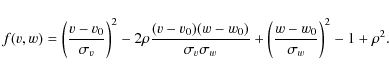
The velocity ellipse of a stellar sample is described by its center (v0, w0), the length of the major and minor axes
From our observations, we compute the velocities
![]() ,
,
![]() ,
for each star at distance d (in pc) and galactic coordinates
(l,b), assuming one more time
that the lack of information on the
los-velocity does not introduce any error larger than
20 km s-1.
,
for each star at distance d (in pc) and galactic coordinates
(l,b), assuming one more time
that the lack of information on the
los-velocity does not introduce any error larger than
20 km s-1.
The use of a velocity ellipse is just a convenient way to
describe a stellar system. We want to explore the evolution
of
![]() over a time-scale of a few
Myr connected to a crossing time of the galactic thin disk.
We consider
over a time-scale of a few
Myr connected to a crossing time of the galactic thin disk.
We consider
![]() stars out of the set of
stars out of the set of
![]() VSC stars that have a height above the galactic
plane
VSC stars that have a height above the galactic
plane ![]() pc. The
pc. The
![]() stars were grouped
into sets of 105 objects in order to get a weight
stars were grouped
into sets of 105 objects in order to get a weight
![]() in our mean estimate for the 5 unknowns
v0, u0,
in our mean estimate for the 5 unknowns
v0, u0, ![]() ,
,
![]() ,
,
![]() of each 105 star group
ordered by increasing mean dynamical time t. This weight of
of each 105 star group
ordered by increasing mean dynamical time t. This weight of
![]() suggests expected mean errors in the estimates of
(V0, W0,
suggests expected mean errors in the estimates of
(V0, W0, ![]() ,
,
![]() )
of 5 km s-1,
since the transverse velocity is
)
of 5 km s-1,
since the transverse velocity is
![]() km s-1.
Figure 15 plots the
km s-1.
Figure 15 plots the
![]() velocity-dispersion ratio, derived
from a weighted least squares fit to f( v,w)=0, for the
various 105-star groups as a function of mean crossing time t for those
groups with
velocity-dispersion ratio, derived
from a weighted least squares fit to f( v,w)=0, for the
various 105-star groups as a function of mean crossing time t for those
groups with ![]() Myr.
The ratio
Myr.
The ratio
![]() measures the anisotropy of the velocity ellipse.
We observe a weak,
but definite correlation between
measures the anisotropy of the velocity ellipse.
We observe a weak,
but definite correlation between
![]() and
and ![]() .
A simple linear fit produces the power law:
.
A simple linear fit produces the power law:
![]() (t in Myr).
The derived power law suggests the existence of some relaxation
mechanism, lasting on the order of
an equipartition time of
t0=6 Myr, in order that the
velocity ellipse be stabilized at its known value of
(t in Myr).
The derived power law suggests the existence of some relaxation
mechanism, lasting on the order of
an equipartition time of
t0=6 Myr, in order that the
velocity ellipse be stabilized at its known value of
![]() for stars in the solar neighborhood (Dehnen & Binney 1998; Binney et al. 2000).
The derived power law exponent of the order of
for stars in the solar neighborhood (Dehnen & Binney 1998; Binney et al. 2000).
The derived power law exponent of the order of
![]() ,
suggests that the relaxation for the selected stellar system
is faster than the increase of total velocity dispersion with age,
which is about a power law with an exponent
,
suggests that the relaxation for the selected stellar system
is faster than the increase of total velocity dispersion with age,
which is about a power law with an exponent
![]() .
.
![\begin{figure}
\par\includegraphics[width=9cm,clip]{10798f15.ps}
\end{figure}](/articles/aa/full_html/2009/33/aa10798-08/img173.png) |
Figure 15:
The ratio
|
| Open with DEXTER | |
We cannot explore further the evolution of the stellar velocity ellipse
given the rudimentary nature of our data. We will only use the
observed correlation of
![]() with dynamical
time
with dynamical
time ![]() 6 Myr to justify a way for selecting candidates for stars
with photospheric activity suspected to have lasted
over that 6 Myr time-scale.
6 Myr to justify a way for selecting candidates for stars
with photospheric activity suspected to have lasted
over that 6 Myr time-scale.
8 Stellar flickering for giant and dwarf stellar candidates
![\begin{figure}
\par\includegraphics[width=9cm,clip]{10798f16.ps}
\end{figure}](/articles/aa/full_html/2009/33/aa10798-08/img174.png) |
Figure 16:
The short-term |
| Open with DEXTER | |
In order to be able to compare stars of similar physical type, we
use for our measure of long-term variability our absolute
magnitude parameter
![]() rather than
rather than ![]() variation in apparent magnitude. We recall
that
variation in apparent magnitude. We recall
that
![]() ,
so the error resulting from
the uncertainty in the distance determination has a small effect on
,
so the error resulting from
the uncertainty in the distance determination has a small effect on
![]() .
It follows that particularly large
.
It follows that particularly large ![]() values are
indicators of possible long-term variability.
values are
indicators of possible long-term variability.
We can now investigate two indicators that are related to possible
changes in stellar luminosity: ![]() ,
which measures
short-term absolute (as well as apparent) magnitude scatter, and
,
which measures
short-term absolute (as well as apparent) magnitude scatter, and
![]() ,
which largely measures the long-term absolute
magnitude scatter. We present in Fig. 16 the relationship
between the observed short-term (
,
which largely measures the long-term absolute
magnitude scatter. We present in Fig. 16 the relationship
between the observed short-term (![]() )
and long-term (
)
and long-term (![]() )
scatter for the 105-star groups of Fig. 15 whose individual
velocity ellipses f(v,w)=0 fit reasonably well
(at a
)
scatter for the 105-star groups of Fig. 15 whose individual
velocity ellipses f(v,w)=0 fit reasonably well
(at a ![]() of 15% level) the derived power law
of 15% level) the derived power law
![]() adopted in the
previous section (
adopted in the
previous section (
![]() ,
,
![]() ,
t =
,
t =
![]() ). Our requirement of a
reasonable power law fit led to the rejection of about
50% of the VSC stars. The resulting set of
). Our requirement of a
reasonable power law fit led to the rejection of about
50% of the VSC stars. The resulting set of
![]() objects are plotted with different symbols for the H-burning and
He-burning stars, as determined by our kinematical classification.
We notice conspicuous correlations between the short-term
objects are plotted with different symbols for the H-burning and
He-burning stars, as determined by our kinematical classification.
We notice conspicuous correlations between the short-term ![]() and long-term
and long-term ![]() scatters that are different for the two types of
stars. The differing relations suggests a variability mechanism
related to stellar radius, probably pulsation (Cox 1980).
scatters that are different for the two types of
stars. The differing relations suggests a variability mechanism
related to stellar radius, probably pulsation (Cox 1980).
Table 3: Distribution of the numbers of probable giants and dwarfs in the VSC according to the correlation level c and at an altitude z above the galactic plane.
![\begin{figure}
\par\includegraphics[width=9cm,clip]{10798f17.ps}
\end{figure}](/articles/aa/full_html/2009/33/aa10798-08/img186.png) |
Figure 17: The statistical HRD for the giant and dwarf candidates that fit the trends shown in Fig. 16 with a probability of 75%. |
| Open with DEXTER | |
We observe that
![]() could be a simple criterion to
help segregate dwarfs and giants. We improve upon this by using the
trends found in Fig. 16 of
could be a simple criterion to
help segregate dwarfs and giants. We improve upon this by using the
trends found in Fig. 16 of
![]() for dwarfs and
for dwarfs and
![]() for giants to improve our classification of the VSC stars into H-burning
or He-burning candidates. We compute a correlation coefficient
c that reflects the probability for a star being part of a Gaussian
distribution around one or the other of the two trend lines,
i.e. either for H-burning or for He-burning candidates,
marked in Fig. 16. This coefficient, which ranges from 0 to 1,
reflects how well correlated are the short-term and
long-term magnitude scatters for a star. Table 3 gives the numbers of stars at different levels of c for the various stellar types as determined from the statistical HRD (WD I = white dwarfs, MS I = main sequence stars, RG I = red giants of Pop. I,
SD II = subdwarfs, RG II = red giants of Pop. II, HB II = blue horizontal branch stars) and at an altitude z above the galactic plane. We suggest that the Pop. I stellar system with
for giants to improve our classification of the VSC stars into H-burning
or He-burning candidates. We compute a correlation coefficient
c that reflects the probability for a star being part of a Gaussian
distribution around one or the other of the two trend lines,
i.e. either for H-burning or for He-burning candidates,
marked in Fig. 16. This coefficient, which ranges from 0 to 1,
reflects how well correlated are the short-term and
long-term magnitude scatters for a star. Table 3 gives the numbers of stars at different levels of c for the various stellar types as determined from the statistical HRD (WD I = white dwarfs, MS I = main sequence stars, RG I = red giants of Pop. I,
SD II = subdwarfs, RG II = red giants of Pop. II, HB II = blue horizontal branch stars) and at an altitude z above the galactic plane. We suggest that the Pop. I stellar system with
![]() and
and
![]()
![]() 100 pc is the most appropriate distance-limited sample in view of the numbers of MS I and RG I candidates.
100 pc is the most appropriate distance-limited sample in view of the numbers of MS I and RG I candidates.
![\begin{figure}
\par\includegraphics[width=9cm,clip]{10798f18.ps}
\end{figure}](/articles/aa/full_html/2009/33/aa10798-08/img191.png) |
Figure 18: The statistical HRD for the possible optical counterparts of X-ray sources. |
| Open with DEXTER | |
It must be remembered that the stars in Fig. 16
are only suspected variables, i.e. there are
both stars that are indeed varying and ones for which
the variability is an artifact of errors in the data. The
(Mb,[B-V]0)-diagram for those objects most likely to
be true variables, i.e. those with
![]() ,
is shown Fig. 17. We immediately see that this statistical HRD shows mostly dwarfs - both Pop. I
and Pop. II - along with some Pop. I red giants; there are
few evolved Pop. II stars (RG II and HB II stars). The
tentative instability strip is marked. We feel that it is
the blue objects in this region, that is those stars with
,
is shown Fig. 17. We immediately see that this statistical HRD shows mostly dwarfs - both Pop. I
and Pop. II - along with some Pop. I red giants; there are
few evolved Pop. II stars (RG II and HB II stars). The
tentative instability strip is marked. We feel that it is
the blue objects in this region, that is those stars with
![]() ,
that have the most probability
of being actual variables. We suggest that these probable
O, B, and A0 stars are the most interesting objects for
follow up studies. This shows the improvement in the classification of
stars compared to Fig. 10 by adding the fitting criterion of
Fig. 16. The suggested instability strip (I.S.) extending from the Blue Horizontal Branch
through the ZAMS and down to the hot WD I candidates is shown.
,
that have the most probability
of being actual variables. We suggest that these probable
O, B, and A0 stars are the most interesting objects for
follow up studies. This shows the improvement in the classification of
stars compared to Fig. 10 by adding the fitting criterion of
Fig. 16. The suggested instability strip (I.S.) extending from the Blue Horizontal Branch
through the ZAMS and down to the hot WD I candidates is shown.
Table 4: List of VSC stellar candidates as possible optical counterparts of known X-ray sources.
The poor time coverage and our restriction that all stars in
the VSC catalog appear on at least three plates (see Sect. 5)
makes identifying long-period variables such as
Mira's more difficult because
of the probability that their large amplitudes caused them to
be too faint to appear on one or more of the three plates of a field.
Therefore, we have focused the test of our selection
procedure on our suspected short-period variables.
We have matched the list of the VSC stars plotted in Fig. 17
with the Rosat All Sky Survey (ROSAT) in order to see
if larger than normal short-term photometric
scatter indeed identifies some known and suspected
variables, in this case known X-ray emitters
suspected to be pre-main sequence stars (PMS).
The typical positional uncertainty
of ROSAT is around 15 arcsec, but for some sources
it is as large as 40 arcsec. We used a
conservative search radius of 15 arcsec
which resulted in 67 possible coincidences that
are presented in Table 4.
It is obvious that some of these
are simply chance since the VSC stars are extracted from a deep
survey down to
![]() and
in some cases the star density makes a coincidence
with a low-accuracy ROSAT position likely. Nevertheless, we were pleased to find that
larger than normal photometric scatter
identifies some known and probable variables, which we classified as Pop. I candidates with
and
in some cases the star density makes a coincidence
with a low-accuracy ROSAT position likely. Nevertheless, we were pleased to find that
larger than normal photometric scatter
identifies some known and probable variables, which we classified as Pop. I candidates with
![]() .
In 13 cases, our star had previously been identified
as the X-ray source:
7 PMSs, 2 CanVen stars, 2 Algol-type stars, one emission-line
star and one BY Dra variable (Caillault 1982).
The only information that
supports any of the other candidates
being the X-ray source is the positional agreement
with the VSC arcsecond precise coordinates.
We plot in Fig. 18 the set of 67 candidates, which seems
to show that a larger than expected
number of stars are bluewards to the Parenago's discontinuity.
We also show in Fig. 18
the lines that border our suspected
instability region (the line on the left
is from the VSC analysis and shown in Fig. 17).
The statistical HRD for the
possible optical counterparts
of X-ray sources with crossing time of the thin disk
.
In 13 cases, our star had previously been identified
as the X-ray source:
7 PMSs, 2 CanVen stars, 2 Algol-type stars, one emission-line
star and one BY Dra variable (Caillault 1982).
The only information that
supports any of the other candidates
being the X-ray source is the positional agreement
with the VSC arcsecond precise coordinates.
We plot in Fig. 18 the set of 67 candidates, which seems
to show that a larger than expected
number of stars are bluewards to the Parenago's discontinuity.
We also show in Fig. 18
the lines that border our suspected
instability region (the line on the left
is from the VSC analysis and shown in Fig. 17).
The statistical HRD for the
possible optical counterparts
of X-ray sources with crossing time of the thin disk ![]() Myr
suggests a lower level for the instability strip suggested in
Fig. 17. In order to say more,
our list of stars with suspected photospheric activity
needs follow-up observations, particularly for the
bluer candidates in order to check our
prediction these stars in a non-quiescent state
and to explore our tentatively-identified
instability strip.
The stars in Table 4 with no specific type archived in Simbad
could be good targets of opportunity
to establish if they are active stars and intrinsic X-ray emitters.
For stars on the main sequence,
two mechanisms are known to be responsible
for the possible X-ray emission. In O and early B-type
stars, the X-rays are
produced by instabilities arising in
stellar winds (Lucy & White 1980; Owocki & Cohen 1999) and in
late-type stars a solar-like magnetic dynamo is
thought to heat and confine hot
coronal plasma which is a tracer of stellar activity (Parker 1955).
Fairly low-mass dwarfs are
known to show anomalous strong activity when they are
rapidly rotating (with periods in the 5-10 day range).
We suggest therefore the observation of v
Myr
suggests a lower level for the instability strip suggested in
Fig. 17. In order to say more,
our list of stars with suspected photospheric activity
needs follow-up observations, particularly for the
bluer candidates in order to check our
prediction these stars in a non-quiescent state
and to explore our tentatively-identified
instability strip.
The stars in Table 4 with no specific type archived in Simbad
could be good targets of opportunity
to establish if they are active stars and intrinsic X-ray emitters.
For stars on the main sequence,
two mechanisms are known to be responsible
for the possible X-ray emission. In O and early B-type
stars, the X-rays are
produced by instabilities arising in
stellar winds (Lucy & White 1980; Owocki & Cohen 1999) and in
late-type stars a solar-like magnetic dynamo is
thought to heat and confine hot
coronal plasma which is a tracer of stellar activity (Parker 1955).
Fairly low-mass dwarfs are
known to show anomalous strong activity when they are
rapidly rotating (with periods in the 5-10 day range).
We suggest therefore the observation of v![]() among these targets to confirm the observed correlation between the blue bright stellar outbursts
and the dynamical crossing time t.
among these targets to confirm the observed correlation between the blue bright stellar outbursts
and the dynamical crossing time t.
9 Does the VSC reveal any true interesting behavior?
We have stressed that we are dealing with only variability indicators -
short-term and long-term magnitude dispersions - for stars tentatively
classified as giants, dwarfs or other types using kinematical
properties. Our results are only statistical in nature in view of the
very rudimentary way we segregate giants from dwarfs in the RPMD.
We used a relation derived from the RPMD between total p.m.
![]() and parallax
and parallax ![]() that follows from the known values
in the solar neighborhood of
that follows from the known values
in the solar neighborhood of ![]() km s-1 if
km s-1 if
![]() and
and ![]() km s-1 if
km s-1 if
![]() (Dehnen & Binney 1998). Then we classify
the VSC stars into different groups based how close a star lies
to one or another of the well-calibrated Pop. I and II ridge-lines.
While this appoach is judged adequate for a quick-look
investigation of a physical mechanism linked to a stellar radius,
such an automated classification procedure will obviously
be misleading in many cases.
(Dehnen & Binney 1998). Then we classify
the VSC stars into different groups based how close a star lies
to one or another of the well-calibrated Pop. I and II ridge-lines.
While this appoach is judged adequate for a quick-look
investigation of a physical mechanism linked to a stellar radius,
such an automated classification procedure will obviously
be misleading in many cases.
We propose ![]() and
and
![]() as possible indicators of variability that can also serve to improve
our classification into H-burning and He-burning stars for
those candidates at an altitude over the galactic plane
as possible indicators of variability that can also serve to improve
our classification into H-burning and He-burning stars for
those candidates at an altitude over the galactic plane
![]() pc. Thus, this work is essentially just
an exploratory analysis to see what might be extracted from data
obtained from a photographic survey that was intended exclusively
for charting purposes. Confirmation and understanding of
our tentative findings will need follow-up observations (Fresneau et al. 2001).
pc. Thus, this work is essentially just
an exploratory analysis to see what might be extracted from data
obtained from a photographic survey that was intended exclusively
for charting purposes. Confirmation and understanding of
our tentative findings will need follow-up observations (Fresneau et al. 2001).
Obviously, our low-accuracy data cannot be used for thorough
analyses. Rather, we have used the data to come up with a
manageable list of targets for further study (Jenkins et al. 2006;
Waelkens et al. 1998). For example, by restricting the interesting
candidates to those VSC stars that meet the criteria
![]() and
and
![]() pc, one
has a target list suitable for checking our observed
correlations between short-term and long-term
magnitude variations. Such a target list
would be very appropriate for follow up using
current all-sky monitoring programs such as ROTSE
(Akerlof 2000; Akerlof et al. 2003) and ASAS (Pojmanski 2004; Wozniak 2004).
pc, one
has a target list suitable for checking our observed
correlations between short-term and long-term
magnitude variations. Such a target list
would be very appropriate for follow up using
current all-sky monitoring programs such as ROTSE
(Akerlof 2000; Akerlof et al. 2003) and ASAS (Pojmanski 2004; Wozniak 2004).
10 Selected areas for monitoring the VSC behavior
The positions in the SOAP, SOGS and VSC catalogs are sufficiently
accurate that the stars are readily identified and hence the
reality of the short-term magnitude variations for given stars
could be readily confirmed using modern epoch surveys
(Barron et al. 2008; Pojmanski & Maciejewski 2004). In order to identify targets
for detailed study, such as photometric or spectroscopic
monitoring (Jenkins et al. 2006), we have prepared two files
suitable for investigating our tentative findings, first
a correlation between flickering and long-term variability
and second a correlation between long-term variability and
galactic plane crossing time
![]() when
when ![]() Myr.
Myr.
The first list has 236797 stars along the galactic equator section
![]() and
and
![]() suitable for monitoring flickering and long-term magnitude
scatter
suitable for monitoring flickering and long-term magnitude
scatter![]() .
The second list has 164691 stars along the galactic meridian segment
.
The second list has 164691 stars along the galactic meridian segment
![]() ,
,
![]()
![]() that is suitable for exploring long-term magnitude scatter as a
function of crossing time. We suggest that crossings of the Sagittarius
Spiral Arm could be investigated by adding los-velocity
information on the targets, such as could be
provided by current observing programs (Minchev & Quillen 2008).
The objects in both lists contain data on galactic thin disk kinematics
(derived from the stars' p.m. components and the statistical
parallaxes),
and we suggest these as potential tracers of the interface
between the thin and thick disks in the solar neighborhood
(Fresneau et al. 2007).
Each target file has for each star the J2000 equatorial
coordinates, p.m. in galactic components (in ''yr-1),
our estimated statistical parallax and its error (in 10
that is suitable for exploring long-term magnitude scatter as a
function of crossing time. We suggest that crossings of the Sagittarius
Spiral Arm could be investigated by adding los-velocity
information on the targets, such as could be
provided by current observing programs (Minchev & Quillen 2008).
The objects in both lists contain data on galactic thin disk kinematics
(derived from the stars' p.m. components and the statistical
parallaxes),
and we suggest these as potential tracers of the interface
between the thin and thick disks in the solar neighborhood
(Fresneau et al. 2007).
Each target file has for each star the J2000 equatorial
coordinates, p.m. in galactic components (in ''yr-1),
our estimated statistical parallax and its error (in 10
![]() ),
apparent V-magnitude (from GSC1.2), mean mb and its scatter
and mean epoch. The files are accessible at
ftp://cdsarc.u-strasbg.fr/incoming/fresneau/havs.
),
apparent V-magnitude (from GSC1.2), mean mb and its scatter
and mean epoch. The files are accessible at
ftp://cdsarc.u-strasbg.fr/incoming/fresneau/havs.
11 Conclusion
The Sydney Observatory Astrographic Program (SOAP) was part of an
extensive photographic survey of the southern sky (Pickering 1903)
that took over 40 years (1892-1932) to complete (White 1988).
Unfortunately, the program lasted too long (Hearnshaw 1996) and
this rich set of data from four decades of observations
has never been fully analyzed. The only results were
positions and rough magnitudes (![]() 0.4) for stars brighter
than 12th mag that were used in the Sydney Observatory's
contributions to the astrographic catalog (Urban et al. 1998)
and a list of double stars noted on the plates
(Barton 1937).
0.4) for stars brighter
than 12th mag that were used in the Sydney Observatory's
contributions to the astrographic catalog (Urban et al. 1998)
and a list of double stars noted on the plates
(Barton 1937).
New measurements of previously unstudied plates has produced a
catalog of
![]() stars (the SOGS), the data for
which is available on-line thanks to the VizieR data mining
system. Present day surveys (such as SDSS, OGLE, DENIS, 2MASS,
and UKIDSS) are plainly superior and photographic surveys
are now obsolete. One might therefore question the value of the
SOGS data, given the low accuracy
(
stars (the SOGS), the data for
which is available on-line thanks to the VizieR data mining
system. Present day surveys (such as SDSS, OGLE, DENIS, 2MASS,
and UKIDSS) are plainly superior and photographic surveys
are now obsolete. One might therefore question the value of the
SOGS data, given the low accuracy
(![]() 0.3 arcsec in equatorial coordinates,
0.3 arcsec in equatorial coordinates, ![]() 0.4 in
derived magnitudes), but the early epoch permits
such things as improving p.m. (Frankowski et al. 2007), separating physical
visual binaries from optical pairs (Lopez 2003; Ficher 1975),
and detecting stellar changes with time scales of
centuries (Lopez 2004). We have applied to one early survey
an automated procedure to identify in a RPMD stellar candidates
of special interest -
in this case ones with interesting photospheric activity.
0.4 in
derived magnitudes), but the early epoch permits
such things as improving p.m. (Frankowski et al. 2007), separating physical
visual binaries from optical pairs (Lopez 2003; Ficher 1975),
and detecting stellar changes with time scales of
centuries (Lopez 2004). We have applied to one early survey
an automated procedure to identify in a RPMD stellar candidates
of special interest -
in this case ones with interesting photospheric activity.
Previous exploratory work has shown that these data can be
used to study stellar kinematics in the Galaxy. Results
were the detection of a density wave linked to the Sagittarius
spiral arm (Fresneau et al. 2005, 2007) and evidence of the
deflection of galactic orbits by the Southern Coalsack
(Fresneau et al. 2003). Our present study suggests evolution of the
stability of the stellar system with time, given that the
![]() ratio of the velocity ellipse
apparently increases from 0.45 up to 0.75 over about 6 Myr.
Further, for this time scale we found a tentative correlation
between photometric flickering and long-term variability
that differs for giants and dwarfs, and can therefore be
used to help segregate stars into these classes.
ratio of the velocity ellipse
apparently increases from 0.45 up to 0.75 over about 6 Myr.
Further, for this time scale we found a tentative correlation
between photometric flickering and long-term variability
that differs for giants and dwarfs, and can therefore be
used to help segregate stars into these classes.
We produced a statistical HRD of suspected variables,
and showed that it can be improved through the observed
scatter of the photometric measures of different
observations of the same star. The result is a set of
![]() potential variable stars that we call
the Variable Sample Catalog (VSC). The catalog
contains objects brighter than about mb=14,
suspected of rapid variations (approximately 30 min
time scale) as well as on longer scales in the years
1892-1932. The stars with
potential variable stars that we call
the Variable Sample Catalog (VSC). The catalog
contains objects brighter than about mb=14,
suspected of rapid variations (approximately 30 min
time scale) as well as on longer scales in the years
1892-1932. The stars with
![]() are considered the most interesting objects for follow up
studies. The catalog is accessible through anonymous
ftp
are considered the most interesting objects for follow up
studies. The catalog is accessible through anonymous
ftp![]() .
The VSC archival material leads to a target list for monitoring
by modern ground-based surveys, especially automated wide-field
programs that observe the sky on a time scale of hours
(Eyer & Blake 2005). Our tentative identification of flickering
effects on moderately faint stars shows that the
systematic study of the archival material
can be valuable (van Genderen et al. 1997), especially along the Galaxy equator.
.
The VSC archival material leads to a target list for monitoring
by modern ground-based surveys, especially automated wide-field
programs that observe the sky on a time scale of hours
(Eyer & Blake 2005). Our tentative identification of flickering
effects on moderately faint stars shows that the
systematic study of the archival material
can be valuable (van Genderen et al. 1997), especially along the Galaxy equator.
Acknowledgements
We thank Christian Motch from Strasbourg astronomical observatory for his advice in the matching process by stellar coordinates of our results with the Rosat All Sky Survey. We thank the referee for his (or her) constructively critical reviews that improved the clarity of our paper.
References
- Akerlof, C. 2000, AJ, 119, 1901 [NASA ADS] [CrossRef] (In the text)
- Akerlof, C. N., Kehoe, R. L., McKay, T. A., et al. 2003, PASP, 115, 132 [NASA ADS] [CrossRef] (In the text)
- Allen, C. W. 1973, Astrophysical Quantities, 3rd edition (The Athlone Press, University of London), Chap. 12 (In the text)
- Andersen, J. 1977, A&AS, 29, 257 [NASA ADS] (In the text)
- Bahcall, J. N., & Soneira, R. M. 1980, ApJS, 44, 73 [NASA ADS] [CrossRef] (In the text)
- Bahcall, J. N., & Casertano, S. 1986, ApJ, 308, 347 [NASA ADS] [CrossRef] (In the text)
- Barron, J. T., Stumm, C., Hogg, D. W., Lang, D., & Roweis, S. 2008, AJ, 135, 414 [NASA ADS] [CrossRef] (In the text)
- Barton, S. G. 1937, Astron. Nachr., 263, 383 [NASA ADS] [CrossRef] (In the text)
- Bash, F. 1986, in The Galaxy and the solar system, ed. R. Smoluchowski, J. N. Bahcall, & M. S. Matthews (University of Arizona Press), 35 (In the text)
- Becker, A. C., Wittman, D. M., Boeshaar, P. C., et al. 2004, ApJ, 611, 418 [NASA ADS] [CrossRef] (In the text)
- Bensby, T., Feltzing, S., & Lundström, I. 2004, A&A, 415, 155 [NASA ADS] [CrossRef] [EDP Sciences] (In the text)
- Bernkopf, J., & Fuhrmann, K. 2006, MNRAS, 369, 673 [NASA ADS] [CrossRef] (In the text)
- Binney, J., et al. 1998a, MNRAS, 288, 365 [NASA ADS]
- Binney, J., & Merrifield, M. 1998, Galactic Astronomy (Princeton, New Jersey, USA: Princeton University Press), Chap. 10.3 (In the text)
- Binney, J., Dehnen, W., & Bertelli, G. 2000, MNRAS, 318, 658 [NASA ADS] [CrossRef] (In the text)
- Caillault, J. P. 1982, AJ, 87, 558 [NASA ADS] [CrossRef] (In the text)
- Chinnici, I. 2008, in La Carte du Ciel, ed. J. Lamy (France: EDP Sciences), 19, Chap. 1 (In the text)
- Chiu, L. T. G. 1980, ApJS, 44, 31 [NASA ADS] [CrossRef] (In the text)
- Cox, J. P. 1980, Theory of stellar pulsations (Princeton, New Jersey, USA: Princeton University Press) (In the text)
- Cuisinier, F., Dehnen, W., Bertelli, G., et al. 1994, A&A, 285, 943 [NASA ADS] (In the text)
- Dehnen, W., & Binney, J. J. 1998, MNRAS, 298, 387 [NASA ADS] [CrossRef] (In the text)
- Dick, W. R., Tucholke, H.-J., Brosche, P., et al. 1993, A&A, 279, 267 [NASA ADS] (In the text)
- Drimmel, R., & Spergel, D. N. 2001, ApJ, 556, 181 [NASA ADS] [CrossRef]
- Ducourant, C., Le Campion, J. F., Rapaport, M., et al. 2006, A&A, 448, 1235 [NASA ADS] [CrossRef] [EDP Sciences] (In the text)
- Eyer, L., & Blake, C. 2005, MNRAS, 358, 38 [NASA ADS] [CrossRef] (In the text)
- Famaey, B., Siebert, A., & Jorissen, A. 2008, A&A, 483, 453 [NASA ADS] [CrossRef] [EDP Sciences] (In the text)
- Ficher, L. 1975, MmRaS, 80, 93 [NASA ADS] (In the text)
- Finch, C. T., Henry, T. J., Subasavage, J. P., Jao, W.-C., & Hambly, N. C. 2007, AJ, 133, 2898 [NASA ADS] [CrossRef] (In the text)
- Frankowski, A., Jancart, S., & Jorissen, A. 2007, A&A, 464, 377 [NASA ADS] [CrossRef] [EDP Sciences] (In the text)
- Fresneau, A. 1990, AJ, 100, 1223 [NASA ADS] [CrossRef] (In the text)
- Fresneau, A. 1994, AJ, 108, 629 [NASA ADS] [CrossRef] (In the text)
- Fresneau, A., Argyle, R. W., Marino, G., & Messina, S. 2001, AJ, 121, 517 [NASA ADS] [CrossRef] (In the text)
- Fresneau, A., Vaughan, A. E., & Argyle, R. W. 2003, AJ, 125, 1519 [NASA ADS] [CrossRef] (In the text)
- Fresneau, A., Vaughan, A. E., & Argyle, R. W. 2005, AJ, 130, 2701 [NASA ADS] [CrossRef] (In the text)
- Fresneau, A., Vaughan, A. E., & Argyle, R. W. 2007, A&A, 469, 1221 [NASA ADS] [CrossRef] [EDP Sciences] (In the text)
- Fuhrmann, K. 2008, MNRAS, 384, 173 [NASA ADS] [CrossRef] (In the text)
- Gautschy, A., & Saio, H. 1995, ARA&A, 33, 75 [NASA ADS] [CrossRef] (In the text)
- Gautschy, A., & Saio, H. 1996, ARA&A, 34, 551 [NASA ADS] [CrossRef] (In the text)
- Geffert, M., Bonnefond, P., Maintz, G., & Guibert, J. 1996, A&AS, 118, 277 [NASA ADS] [CrossRef] [EDP Sciences] (In the text)
- van Genderen, A. M., Sterken, C., & de Groot, M. 1997, A&A, 318, 81 [NASA ADS] (In the text)
- Gilmore, R., & Reid, N. 1983, MNRAS, 202, 1025 [NASA ADS] (In the text)
- Gilmore, G., et al. 1989, The Milky Way as a Galaxy (Mill Valley CA: University Science Books), Chap. 9 (In the text)
- Gliese, W., & Jahreiss, H. 1980, A&A, 85, 350 [NASA ADS] (In the text)
- Goldreich, P., & Lynden Bell, D. 1965, MNRAS, 130, 125 [NASA ADS] (In the text)
- Hammersley, P. L., Garzon, F., Mahoney, T., & Calbet, X. 1995, MNRAS, 273, 206 [NASA ADS]
- Hearnshaw, J. B. 1996, The measurement of starlight (Cambridge, UK: Cambridge University Press) (In the text)
- Herbst, W., & Sawyer, D. L. 1981, AJ, 243, 935 [NASA ADS] [CrossRef] (In the text)
- Hertzsprung, E. 1929, MNRAS, 89, 660 (In the text)
- von Hippel, T., Storrie-Lombardi, L. J., Storrie-Lombardi, M. C., & Irwin, M. J. 1994, MNRAS, 269, 97 [NASA ADS] (In the text)
- Hog, E., Fabricius, C., Makarov, V. V., et al. 2000, A&A, 355, L27 [NASA ADS] (In the text)
- Holmberg, J., Nordström, B., & Andersen, J. 2007, A&A, 475, 519 [NASA ADS] [CrossRef] [EDP Sciences] (In the text)
- Ivezic, Z., Sesar, B., Juric, M., et al. 2008, ApJ, 684, 287 [NASA ADS] [CrossRef] (In the text)
- Jenkins, A., & Binney, J. 1990, MNRAS, 245, 305 [NASA ADS] (In the text)
- Jenkins, J. S., Jones, H. R. A., Tinney, C. G., et al. 2006, MNRAS, 372, 163 [NASA ADS] [CrossRef] (In the text)
- Johnson, H. L., & Morgan, W. W. 1953, ApJ, 117, 313 [NASA ADS] [CrossRef] (In the text)
- Jones, E. M. 1972, ApJ, 173, 671 [NASA ADS] [CrossRef] (In the text)
- Juric, M., Ivezic, Z., Brooks, A., et al. 2008, ApJ, 673, 864 [NASA ADS] [CrossRef] (In the text)
- Kibblewhite, E. J., et al. 1984, Astronomical Microdensitometry Conference, ed. D.A. Klinglesmith (Washington: NASA), 277 (In the text)
- Kilic, M., Munn, J. A., Harris, H. C., et al. 2006, AJ, 131, 582 [NASA ADS] [CrossRef] (In the text)
- Kleinmann, S. G. 1992, Robotic telescopes in the 1990, ASP Conf. Ser., 34, 203 [NASA ADS] (In the text)
- Lacey, C. G. 1984, MNRAS, 208, 687 [NASA ADS] (In the text)
- Lamareille, Thiévin, J., Fournis, B., et al. 2003, A&A, 402, 395 [NASA ADS] [CrossRef] [EDP Sciences] (In the text)
- Larsen, J. A., & Humphreys, R. M. 2003, AJ, 125, 1958 [NASA ADS] [CrossRef] (In the text)
- Lasker, B. M., Sturch, C. R., McLean, B. J., et al. 1990, AJ, 99, 2019 [NASA ADS] [CrossRef] (In the text)
- Lasker, B. M., Lattanzi, M. G., McLean, B. J., et al. 2008, AJ, 136, 735 [NASA ADS] [CrossRef] (In the text)
- van Leeuwen, F. 2007, A&A, 474, 653 [NASA ADS] [CrossRef] [EDP Sciences] (In the text)
- Lopez, C. E. 2003, in Astronomy in Latin America ADeLA Publications Series, ed. R. Teixeira et al., 1, 191 (In the text)
- Lopez, C. E. 2004, Astrophysics and Space Science, 290, 439 [NASA ADS] [CrossRef] (In the text)
- Lucy, L. B., & White, R. L., 1980, ApJ, 241, 300 [NASA ADS] [CrossRef] (In the text)
- Luyten, W. 1922, Lick Observatory Bulletin, Vol. X, 135 (In the text)
- Luyten, W. J. 1977, in The HR diagram, ed. A. G. Davis Philip, & D. S. Hayes (Dordrecht: D. Reidel), IAU Symp., 80, 63 (In the text)
- Marshall, D. J., Robin, A. C., Reylé, C., Schultheis, M., & Picaud, S. 2006, A&A, 453, 635 [NASA ADS] [CrossRef] [EDP Sciences] (In the text)
- Minchev, I., & Quillen, A. C. 2008, MNRAS, 386, 1579 [NASA ADS] [CrossRef] (In the text)
- Munn, J. A., Monet, D. G., Levine, S. E., et al. 2004, AJ, 127, 3034 [NASA ADS] [CrossRef] (In the text)
- Nordstöm, Mayor, M., Andersen, J., et al. 2004, A&A, 418, 989 [NASA ADS] [CrossRef] [EDP Sciences] (In the text)
- Ortiz-Gil, A., Hiesgen, M., & Brosche, P. 1998, A&AS, 128, 621 [NASA ADS] [CrossRef] [EDP Sciences] (In the text)
- Owocki, S. P., & Cohen, D. H. 1999, ApJ, 520, 833 [NASA ADS] [CrossRef] (In the text)
- Pace, G., & Pasquini, L. 2004, A&A, 426, 1021 [NASA ADS] [CrossRef] [EDP Sciences] (In the text)
- Parker, E. N. 1955, ApJ, 122, 293 [NASA ADS] [CrossRef] (In the text)
- Perryman, M. 2009, Astronomical Application of Astrometry (Cambridge University Press), Sect. 5.2.5 (In the text)
- Perrymann, M. A. C., et al. 2000, A&A, 369, 339 [NASA ADS] [CrossRef] (In the text)
- Pickering, E. C. 1903, ApJ, 18, 70 [NASA ADS] [CrossRef] (In the text)
- Pojmanski, G. 2004, Astron. Nachr., 325, 553 [NASA ADS] [CrossRef] (In the text)
- Pojmanski, G., & Maciejewski, G. 2004, Acta Astron., 54, 153 [NASA ADS] [CrossRef] (In the text)
- Roman, N. 1950, ApJ, 112, 554 [NASA ADS] [CrossRef] (In the text)
- Russell, H. C. 1891, MNRAS, 51, 495 [NASA ADS] (In the text)
- Sesar, B., Ivezic, Z., Lupton, R. H., et al. 2007, AJ, 134, 2236 [NASA ADS] [CrossRef] (In the text)
- Siegel, M. H., Majewski, S. R., Reid, I. N., & Thompson, I. B. 2002, ApJ, 578, 151 [NASA ADS] [CrossRef] (In the text)
- Skrutskie, M. F., Cutri, R. M., Stiening, R., et al. 2006, AJ, 131, 1163 [NASA ADS] [CrossRef] (In the text)
- Smart, R. L., Lattanzi, M. G., Jahreiß, H., Bucciarelli, B., & Massone, G. 2007, A&A, 464, 787 [NASA ADS] [CrossRef] [EDP Sciences] (In the text)
- Sowell, J. R., Trippe, M., Caballero-Nieves, S. M., & Houk, N. 2007, AJ, 134, 1089 [NASA ADS] [CrossRef] (In the text)
- Spitzer, L., & Schwarzschild, M. 1953, ApJ, 118, 106 [NASA ADS] [CrossRef] (In the text)
- Stothers, R. B. 1998, MNRAS, 300, 1098 [NASA ADS] [CrossRef]
- Strand, K. Aa. 1963, Basic Astronomical Data of Stars and Stellar Systems (University of Chicago Press), Vol. III, Chap. 20 (In the text)
- Toomre, A. 1964, ApJ, 139, 1217 [NASA ADS] [CrossRef] (In the text)
- Torbett, M. V. 1986, MNRAS, 223, 885 [NASA ADS]
- Urban, S. E., Corbin, T. E., Wycoff, G. L., et al. 1998, AJ, 115, 1212 [NASA ADS] [CrossRef] (In the text)
- Waelkens, C., Aerts, C., Kestens, E., Grenon, M., & Eyer, L. 1998, A&A, 330, 215 [NASA ADS] (In the text)
- West, A. A., Bochanski, J. J., & Hawley, S. L. 2006, AJ, 132, 2507 [NASA ADS] [CrossRef] (In the text)
- West, A., Hawley, S. L., Bochanski, J. J., et al. 2008, AJ, 135, 785 [NASA ADS] [CrossRef] (In the text)
- White, G. L. 1988, in Mapping the sky (Kluwer Academic Publishers), IAU Symp., 133, 45 (In the text)
- Wozniak, P. P. 2004, AJ, 127, 2436 [NASA ADS] [CrossRef] (In the text)
Footnotes
- ... Survey
- Data files are only available in electronic form at the CDS via anonymous ftp to cdsarc.u-strasbg.fr (130.79.128.5) or via http://cdsweb.u-strasbg.fr/cgi-bin/qcat?J/A+A/503/1023
- ... system
- http://vizier.u-strasbg.fr/viz-bin/VizieR
- ...
ftp
- ftp://cdsarc.u-strasbg.fr/incoming/fresneau/havs/vsc.dat
- ... effects
- We note that the Sun, with an altitude of 15 pc (Binney et al. 1998a; Hammersley et al. 1995; Drimmel & Spergel 2001) above the galactic plane and an upwards velocity of 9 km s-1 (Stothers 1998; Torbett 1986) crossed the galactic equator about 1.5 Myr ago.
- ... scatter
- ftp://cdsarc.u-strasbg.fr/incoming/fresneau/havs/equator.dat
- ...
![$b\in[-64^\circ,-7^\circ]$](/articles/aa/full_html/2009/33/aa10798-08/img20.png)
- ftp://cdsarc.u-strasbg.fr/incoming/fresneau/havs/meridian.dat
- ...
ftp
- ftp://cdsarc.u-strasbg.fr/incoming/fresneau/havs/vsc.dat
All Tables
Table 1:
Distribution of the B1900.0 centers of the 1400
![]() fields of the Sydney Observatory Astrographic Program.
fields of the Sydney Observatory Astrographic Program.
Table 2:
Distribution of the numbers of stars fainter than
mb=10 in the statistical HRD of Fig. 10 separated
into groups according to ![]() and
and ![]() levels.
levels.
Table 3: Distribution of the numbers of probable giants and dwarfs in the VSC according to the correlation level c and at an altitude z above the galactic plane.
Table 4: List of VSC stellar candidates as possible optical counterparts of known X-ray sources.
All Figures
| |
Figure 1: The mean error in measured magnitude as a function of apparent magnitude mb. |
| Open with DEXTER | |
| In the text | |
| |
Figure 2: The cumulative frequency of the magnitude errors is plotted for observations performed after and before 1915. |
| Open with DEXTER | |
| In the text | |
| |
Figure 3:
The numbers N of foreground and background stars as function of the apparent magnitude
|
| Open with DEXTER | |
| In the text | |
| |
Figure 4:
Number N of stars with
|
| Open with DEXTER | |
| In the text | |
| |
Figure 5: The relation between absolute magnitudes from objective prism spectra (MB) and the RPM quantity Hb for a set of 104 stars in SOGS. |
| Open with DEXTER | |
| In the text | |
| |
Figure 6: The absolute magnitude Mb derived from the calibration of Fig. 5, is plotted as function of the colour index (b-V). |
| Open with DEXTER | |
| In the text | |
| |
Figure 7:
Numbers N of foreground (
|
| Open with DEXTER | |
| In the text | |
| |
Figure 8:
Numbers N of stars (
|
| Open with DEXTER | |
| In the text | |
| |
Figure 9: The reduced proper motion diagram (RPMD) [Hb,(b-V)] of the VSC stars that results by converting to a Mb, (B-V)0 diagram by applying the relations Mb=0.86 Hb-3.6 and (B-V)0=0.82(b-V)+0.26 as determined from Figs. 5 and 6. |
| Open with DEXTER | |
| In the text | |
| |
Figure 10:
The statistical HRD for the Variable Sample Catalogue
(VSC) set of
|
| Open with DEXTER | |
| In the text | |
| |
Figure 11:
Short-term |
| Open with DEXTER | |
| In the text | |
![\begin{figure}
\par\includegraphics[width=9cm,clip]{10798f12.ps}
\end{figure}](/articles/aa/full_html/2009/33/aa10798-08/img124.png) |
Figure 12:
Short-term |
| Open with DEXTER | |
| In the text | |
![\begin{figure}
\par\includegraphics[width=9cm,clip]{10798f13.ps}
\end{figure}](/articles/aa/full_html/2009/33/aa10798-08/img125.png) |
Figure 13:
Short-term |
| Open with DEXTER | |
| In the text | |
| |
Figure 14:
Short-term |
| Open with DEXTER | |
| In the text | |
| |
Figure 15:
The ratio
|
| Open with DEXTER | |
| In the text | |
| |
Figure 16:
The short-term |
| Open with DEXTER | |
| In the text | |
| |
Figure 17: The statistical HRD for the giant and dwarf candidates that fit the trends shown in Fig. 16 with a probability of 75%. |
| Open with DEXTER | |
| In the text | |
| |
Figure 18: The statistical HRD for the possible optical counterparts of X-ray sources. |
| Open with DEXTER | |
| In the text | |
Copyright ESO 2009
Current usage metrics show cumulative count of Article Views (full-text article views including HTML views, PDF and ePub downloads, according to the available data) and Abstracts Views on Vision4Press platform.
Data correspond to usage on the plateform after 2015. The current usage metrics is available 48-96 hours after online publication and is updated daily on week days.
Initial download of the metrics may take a while.