| Issue |
A&A
Volume 503, Number 2, August IV 2009
|
|
|---|---|---|
| Page(s) | 521 - 531 | |
| Section | Stellar structure and evolution | |
| DOI | https://doi.org/10.1051/0004-6361/200912351 | |
| Published online | 02 July 2009 | |
Asteroseismology and interferometry of the red giant star  Ophiuchi
A. Mazumdar1,2,3 - A. Mérand4,5 - P. Demarque2 - P. Kervella6 - C. Barban6,1 - F. Baudin7 - V. Coudé du Foresto6 - C. Farrington5 - P. J. Goldfinger5 - M.-J. Goupil6 - E. Josselin8 - R. Kuschnig9 - H. A. McAlister5 - J. Matthews10 - S. T. Ridgway11 - J. Sturmann5 - L. Sturmann5 - T. A. ten Brummelaar5 - N. Turner5
1 - Instituut voor Sterrenkunde, Katholieke Universiteit,
200D Celestijnenlaan, 3001 Leuven, Belgium
2 - Astronomy Department, Yale University, PO Box 208101, New Haven CT 06520-8101, USA
3 - Homi Bhabha Centre for Science Education, TIFR,
V. N. Purav Marg, Mankhurd, Mumbai 400088, India
4 - European Southern Observatory, Alonso de Córdova 3107, Casilla 19001, Santiago 19, Chile
5 - Center for High Angular Resolution Astronomy, Georgia State University, PO Box 3965, Atlanta, Georgia 30302-3965, USA
6 - LESIA, Observatoire de Paris, CNRS UMR 8109, UPMC, Université Paris Diderot, 5 Place Jules Janssen, 92195 Meudon, France
7 - Institut d'Astrophysique Spatiale, CNRS/Université Paris XI UMR 8617, 91405 Orsay Cedex, France
8 - GRAAL, Université Montpellier II, CNRS UMR 5024, 34095 Montpellier Cedex 05, France
9 -
Institut für Astronomie, Universität Wien, Türkenschanzstrasse 17, 1180 Vienna, Austria
10 - Department of Physics & Astronomy, University of British Columbia, 6224 Agricultural Road, Vancouver V6T 1Z1, Canada
11 - National Optical Astronomy Observatories, 950 North Cherry Avenue, Tucson, AZ 85719, USA
Received 20 April 2009 / Accepted 10 June 2009
Abstract
The GIII red giant star
![]() has been found to exhibit several modes of oscillation by the MOST mission. We interpret the observed frequencies of oscillation in terms of theoretical radial p-mode frequencies of stellar models. Evolutionary models of this star, in
both shell H-burning and core He-burning phases of evolution, are
constructed using as constraints a combination of measurements from
classical ground-based observations (for luminosity, temperature, and
chemical composition) and seismic observations from MOST. Radial
frequencies of models in either evolutionary phase can reproduce the
observed frequency spectrum of
has been found to exhibit several modes of oscillation by the MOST mission. We interpret the observed frequencies of oscillation in terms of theoretical radial p-mode frequencies of stellar models. Evolutionary models of this star, in
both shell H-burning and core He-burning phases of evolution, are
constructed using as constraints a combination of measurements from
classical ground-based observations (for luminosity, temperature, and
chemical composition) and seismic observations from MOST. Radial
frequencies of models in either evolutionary phase can reproduce the
observed frequency spectrum of
![]() almost equally well. The
best-fit models indicate a mass in the range of
almost equally well. The
best-fit models indicate a mass in the range of
![]() with radius of
with radius of
![]() .
We also obtain an independent estimate of the radius of
.
We also obtain an independent estimate of the radius of
![]() with highly accurate interferometric observations in the infrared K' band, using the CHARA/FLUOR instrument. The measured limb-darkened disk angular diameter of
with highly accurate interferometric observations in the infrared K' band, using the CHARA/FLUOR instrument. The measured limb-darkened disk angular diameter of
![]() is
is
![]() mas. Together with the Hipparcos parallax, this translates into a photospheric radius of
mas. Together with the Hipparcos parallax, this translates into a photospheric radius of
![]() .
The radius obtained from the asteroseismic analysis matches the interferometric value quite closely even though the radius was not constrained during the modelling.
.
The radius obtained from the asteroseismic analysis matches the interferometric value quite closely even though the radius was not constrained during the modelling.
Key words: stars: individual: ![]() Ophiuchi - stars: oscillations - stars: interiors - stars: fundamental parameters - techniques: interferometric
Ophiuchi - stars: oscillations - stars: interiors - stars: fundamental parameters - techniques: interferometric
1 Introduction
Asteroseismology of red giant stars has, in recent years, taken a leap forward with the discovery of pulsations in several G- and K-type giant stars, both from the ground (Frandsen et al. 2002; de Ridder et al. 2006) and from space
(Hekker et al. 2008; Kallinger et al. 2008b; Barban et al. 2007). Oscillations in the G giant
![]() Oph (HD 146791, HR 6075, HIP 79882) were first detected in spectroscopic observations from the ground (de Ridder et al. 2006), although the average large separation could not be distinguished between two possible values because of the daily alias problem. Subsequent observations by the MOST satellite (Walker et al. 2003) led to the discovery of at least 9 radial modes with an average large separation of
Oph (HD 146791, HR 6075, HIP 79882) were first detected in spectroscopic observations from the ground (de Ridder et al. 2006), although the average large separation could not be distinguished between two possible values because of the daily alias problem. Subsequent observations by the MOST satellite (Walker et al. 2003) led to the discovery of at least 9 radial modes with an average large separation of
![]() (Barban et al. 2007).
(Barban et al. 2007).
This work makes an attempt to interpret the observed frequencies of
![]() in terms of adiabatic oscillation modes of stellar models in
the relevant part of the HR diagram. We constructed red giant models in which
the luminosity is provided by either hydrogen burning in a shell outside
the helium core, or both shell hydrogen burning and core helium burning.
We make quantitative comparisons of these models to the MOST frequencies
of
in terms of adiabatic oscillation modes of stellar models in
the relevant part of the HR diagram. We constructed red giant models in which
the luminosity is provided by either hydrogen burning in a shell outside
the helium core, or both shell hydrogen burning and core helium burning.
We make quantitative comparisons of these models to the MOST frequencies
of
![]() to determine the stellar parameters like mass, age, radius,
and chemical composition. Kallinger et al. (2008a) have earlier presented stellar
models in the shell hydrogen-burning phase for
to determine the stellar parameters like mass, age, radius,
and chemical composition. Kallinger et al. (2008a) have earlier presented stellar
models in the shell hydrogen-burning phase for
![]() ,
based on
asteroseismic data. A similar study of oscillations in the red giant
,
based on
asteroseismic data. A similar study of oscillations in the red giant
![]() Hya in terms of helium burning models was carried out by
Christensen-Dalsgaard (2004).
Hya in terms of helium burning models was carried out by
Christensen-Dalsgaard (2004).
Interferometric measurements of stellar radii are particularly
discriminating for models, in particular when combined with
asteroseismic frequencies, as noticed, for instance, by
Creevey et al. (2007) and Cunha et al. (2007). In this work we report on a new
interferometric determination of the radius of
![]() .
While the direct
measurement of the radius of a red giant is a useful result in itself,
for
.
While the direct
measurement of the radius of a red giant is a useful result in itself,
for
![]() it provides the first opportunity of testing the relevance
of theoretical models for red giants that have been calibrated with
asteroseismic input. In this study, neither did we use the
interferometric radius as an input to the modelling, nor did the
interferometric analysis draw upon the asteroseismic information in any
way. Thus the radius of the stellar models that fit the seismic data
best can be tested against the independently measured interferometric
radius.
it provides the first opportunity of testing the relevance
of theoretical models for red giants that have been calibrated with
asteroseismic input. In this study, neither did we use the
interferometric radius as an input to the modelling, nor did the
interferometric analysis draw upon the asteroseismic information in any
way. Thus the radius of the stellar models that fit the seismic data
best can be tested against the independently measured interferometric
radius.
In Sect. 2 we describe the details of the stellar models that we constructed and in Sect. 3 we compare the theoretical frequencies obtained from these models with the observed MOST frequencies. In Sect. 4, we present our new interferometric measurement of the angular diameter of
![]() .
In Sect. 5 we compare the radii of our best seismic models with the interferometric measurement, and discuss our results with similar studies carried out earlier.
.
In Sect. 5 we compare the radii of our best seismic models with the interferometric measurement, and discuss our results with similar studies carried out earlier.
2 Stellar models and theoretical frequencies
We constructed a grid of stellar models with various input parameters using the Yale Rotating Evolutionary Code (YREC) (Guenther et al. 1992). This code is capable of producing consistent stellar models for low mass giant stars both in the shell H-burning phase and the core He-burning phase (Demarque et al. 2008). We describe these two sets of models below. The radial and nonradial pulsation frequencies of each model are calculated by the oscillation code JIG (Guenther 1994).
2.1 Input physics
The models use the latest OPAL equation of state (Rogers & Nayfonov 2002) and OPAL opacities (Iglesias & Rogers 1996), supplemented by the low temperature
opacities of Ferguson et al. (2005). The nuclear reaction rates from
Bahcall & Pinsonneault (1992) are used. Diffusion of helium and heavy elements have
been ignored in the post-main sequence phase of evolution. This is
reasonable, since dredge-up by the deep convective envelope present in
red giants would mask any effect of diffusion of elements in early
phases. The current treatment of convection in the models is through the
standard mixing length theory (Böhm-Vitense 1958), which does not properly
include the effects of turbulence in the outer layers, and this might
substantially affect the frequencies of oscillation (see
e.g., Straka et al. 2007). Fortunately, the uncertainty induced in the large
separations is much less than in the actual frequencies themselves.
Mass loss on the giant branch was not included in the calculations. Most
of the mass loss is believed to take place quiescently as the star
approaches the tip of the giant branch, as is the case in the commonly
adopted Reimers (1977) formulation (Yi et al. 2003). Such mass loss does
not affect the thermodynamics of the deep interior appreciably. Most importantly, it takes place at high luminosities, beyond the luminosity of
![]() on the giant branch. The neutrino losses in the core were taken from the work of Itoh et al. (1989).
on the giant branch. The neutrino losses in the core were taken from the work of Itoh et al. (1989).
2.2 Range of parameters
The range of input parameters chosen for the models is dictated by the
position of
![]() on the HR diagram and its estimated chemical
composition. The values of effective temperature (
on the HR diagram and its estimated chemical
composition. The values of effective temperature (
![]() ), luminosity (
), luminosity (
![]() ), and
metallicity (
), and
metallicity (
![]() )
are adopted from
de Ridder et al. (2006), who have already carried out a detailed survey of
these parameters from the literature. Tracks were constructed for
different (Y0, Z0) combinations with Y0 ranging from 0.255 to
0.280, and Z0 ranging from 0.012 to 0.015, corresponding to
)
are adopted from
de Ridder et al. (2006), who have already carried out a detailed survey of
these parameters from the literature. Tracks were constructed for
different (Y0, Z0) combinations with Y0 ranging from 0.255 to
0.280, and Z0 ranging from 0.012 to 0.015, corresponding to
![]() .
We adopted the solar abundances as given by
Grevesse & Sauval (1998) in converting
.
We adopted the solar abundances as given by
Grevesse & Sauval (1998) in converting
![]() to Z values.
to Z values.
For each of these combinations, two values of the mixing length
parameter ![]() (the ratio of mixing length to local pressure scale height) have been used: 1.6 and 1.8. Note that using a similar version of YREC and input physics, Kallinger et al. (2008a) used
(the ratio of mixing length to local pressure scale height) have been used: 1.6 and 1.8. Note that using a similar version of YREC and input physics, Kallinger et al. (2008a) used
![]() in their study of
in their study of
![]() .
This is the value of
.
This is the value of ![]() adopted by Yi et al. (2003) for the standard solar model calibration. The radii of red giant models depend sensitively on the choice of
adopted by Yi et al. (2003) for the standard solar model calibration. The radii of red giant models depend sensitively on the choice of ![]() .
.
For each (Y0, Z0, ![]() ), the mass has been varied between 1.8 and 2.4
), the mass has been varied between 1.8 and 2.4
![]() to check for overlap in the box. In most models,
overshoot at the edge of the convective core present on the main
sequence was assumed to have negligible effect on the advanced
evolution. A few models were constructed with overshoot of 0.2 times the pressure scale height at the convective core edge. Because the size of the convective core is not too large in this mass range, the overall structural effect of core overshoot is modest; but evolutionary timescales are slightly increased when core overshoot is taken into
account (Demarque et al. 2004).
to check for overlap in the box. In most models,
overshoot at the edge of the convective core present on the main
sequence was assumed to have negligible effect on the advanced
evolution. A few models were constructed with overshoot of 0.2 times the pressure scale height at the convective core edge. Because the size of the convective core is not too large in this mass range, the overall structural effect of core overshoot is modest; but evolutionary timescales are slightly increased when core overshoot is taken into
account (Demarque et al. 2004).
2.3 Shell H-burning models
Our first set of models for
![]() are on the ascending red giant
branch. These models are characterised by an inert helium core
surrounded by a thin hydrogen burning shell. The mass of the shell
varies between
are on the ascending red giant
branch. These models are characterised by an inert helium core
surrounded by a thin hydrogen burning shell. The mass of the shell
varies between
![]() and
and
![]() depending on the mass and age. The mass of the shell decreases as the star ascends the red giant
branch. We concentrate on models that lie within the
depending on the mass and age. The mass of the shell decreases as the star ascends the red giant
branch. We concentrate on models that lie within the
![]() box on the HR diagram. For each evolutionary track that traverses the box, several models at slightly different ages are constructed so as to span the box. The theoretical frequencies of these models are compared to the observed
frequencies of
box on the HR diagram. For each evolutionary track that traverses the box, several models at slightly different ages are constructed so as to span the box. The theoretical frequencies of these models are compared to the observed
frequencies of
![]() in Sect. 3.
in Sect. 3.
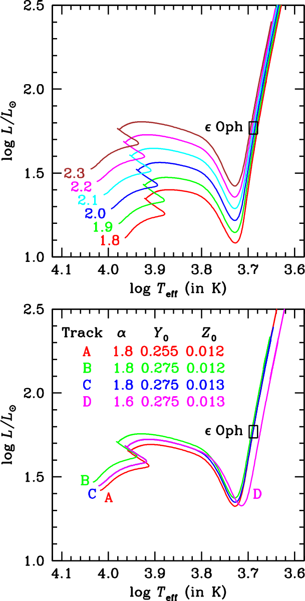 |
Figure 1:
Stellar evolutionary tracks from the ZAMS to the shell H-burning RGB are shown with respect to the position of
|
| Open with DEXTER | |
Each evolutionary track was started in the pre-main sequence phase and evolved continuously through core hydrogen burning and eventually shell hydrogen burning along the giant branch. Some of the tracks are plotted in the HR diagram in Fig. 1, together with the
![]() error box. The size of this box is such that the range of mass of models with
a given set of (Y0, Z0) and
error box. The size of this box is such that the range of mass of models with
a given set of (Y0, Z0) and ![]() values that pass through the box is
values that pass through the box is ![]()
![]() (see top panel of Fig. 1).
Typically, the mass lies between
(see top panel of Fig. 1).
Typically, the mass lies between
![]() and
and
![]() ,
depending on the values of the other parameters. The shift in the tracks with these parameters is also significant (see bottom panel of Fig. 1). Since the outer convective layer of stars in this mass range is extremely thin during the main sequence phase, the tracks with different values of
,
depending on the values of the other parameters. The shift in the tracks with these parameters is also significant (see bottom panel of Fig. 1). Since the outer convective layer of stars in this mass range is extremely thin during the main sequence phase, the tracks with different values of ![]() are almost identical in that phase (e.g., tracks C and D in Fig. 1). But the shift of
the track on the giant branch is significant because of the extended convective envelope. In most cases in this study, however, frequencies of models inside the
are almost identical in that phase (e.g., tracks C and D in Fig. 1). But the shift of
the track on the giant branch is significant because of the extended convective envelope. In most cases in this study, however, frequencies of models inside the
![]() box with
box with
![]() had a poor match with the observed frequencies. Since the tracks move redwards with decreasing
had a poor match with the observed frequencies. Since the tracks move redwards with decreasing ![]() ,
this can be traced to higher mass (and hence larger radii inside the box) of the
,
this can be traced to higher mass (and hence larger radii inside the box) of the
![]() models compared to the
models compared to the
![]() models. Keeping in mind the adopted range of
models. Keeping in mind the adopted range of
![]() for the star, the metallicity of the initial model can only be varied between 0.012 and 0.015 with corresponding appropriate change of initial
helium abundance between 0.255 and 0.280 to span the entire
for the star, the metallicity of the initial model can only be varied between 0.012 and 0.015 with corresponding appropriate change of initial
helium abundance between 0.255 and 0.280 to span the entire
![]() box on the HR diagram.
box on the HR diagram.
2.4 Core He-burning models
The second set of models are in a later stage of evolution than the
first. These models have helium burning in the core of the star.
Hydrogen burning in a thin shell outside the core is also present.
Considering the adopted metallicity value for
![]() ,
these models
represent the so-called ``red clump'' stars, rather than metal-poor
horizontal branch stars. Indeed, the evolutionary tracks of the models
that we constructed lie very close to the red giant branch, and
therefore, overlap with the error box of
,
these models
represent the so-called ``red clump'' stars, rather than metal-poor
horizontal branch stars. Indeed, the evolutionary tracks of the models
that we constructed lie very close to the red giant branch, and
therefore, overlap with the error box of
![]() on the HR diagram.
Figure 2 illustrates these tracks in the HR diagram.
on the HR diagram.
Figure 2 illustrates these tracks in the HR diagram.
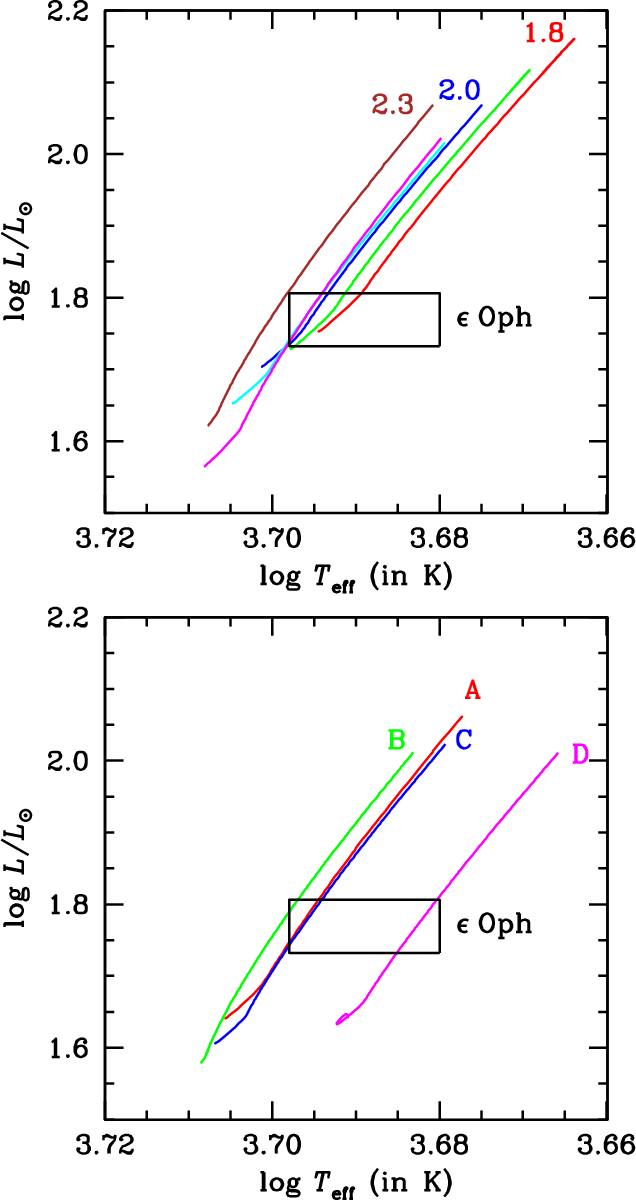 |
Figure 2:
Stellar evolutionary tracks from the ZAHB to the end of He-burning main sequence are shown with respect to the position of
|
| Open with DEXTER | |
For the range of chemical composition used in our models, it turns out that the helium ignition in the core at the tip of the red giant branch takes place under degenerate conditions for the lower mass stars (
![]() ). This is the well-known ``helium flash'' mechanism first studied by Schwarzschild & Härm (1962).
). This is the well-known ``helium flash'' mechanism first studied by Schwarzschild & Härm (1962).
For stars of slightly higher mass (
![]() ), however, the core is not degenerate at the instant helium burning temperatures are reached, and therefore, helium ignition takes place in a controlled fashion. In this latter case, it is numerically easy to continue the
evolution of the model past the tip of the red giant branch, and onto the red clump phase.
), however, the core is not degenerate at the instant helium burning temperatures are reached, and therefore, helium ignition takes place in a controlled fashion. In this latter case, it is numerically easy to continue the
evolution of the model past the tip of the red giant branch, and onto the red clump phase.
For the helium flash scenario, however, the numerical stability of the evolution code at the tip of the giant branch is far less, and only a computationally expensive algorithm involving subtle handling of various parameters can guide the model past the runaway helium ignition process and settle it onto a stable phase of helium burning (Demarque & Mengel 1971). Piersanti et al. (2004) have demonstrated that even for stars which undergo a violent helium flash, the subsequent evolution of a model on the helium-burning main sequence, i.e., once stable core helium burning has been established, is not very sensitive to the prior history of helium ignition. Specifically, the behaviour of models which have been evolved from appropriate zero age horizontal branch (ZAHB) models with quiescent helium burning in the core is remarkably similar to that of models which have been actually evolved through the helium flash phenomenon. Of course, the make-up of the ZAHB model is crucial - it must reflect the properties of a model that has settled on the helium-burning main sequence after having gone through the helium flash. The critical factor in this starting model, apart from the total mass and the chemical composition at the tip of the giant branch, is the mass of the helium core. Hydrodynamical studies in 2D (Cole & Deupree 1983) and 3D (Mocàk et al. 2009) confirm this picture, except for possible second order mixing effects due to turbulent overshoot at the convective-radiative interface, which cannot, at this point, be estimated precisely.
For the low mass models we have, therefore, followed the approach of circumventing the numerical difficulties encountered in handling the helium flash, as done by most authors (e.g., Sweigart 1987; Lee & Demarque 1990). For each mass and chemical composition evolution was continued on the red giant branch till the onset of helium flash. The evolution of the red clump model was then re-started from a ZAHB model of the same total mass with identical chemical composition and helium core mass as the corresponding model at the onset of helium flash at the tip of the red giant branch.
Figure 3 illustrates the behaviour of the central regions of a 2
![]() model near the tip of the giant branch, where helium ignition takes place. The four panels describe the change, as a function of time, or equivalently, as a function of maximum temperature in the star,
model near the tip of the giant branch, where helium ignition takes place. The four panels describe the change, as a function of time, or equivalently, as a function of maximum temperature in the star,
![]() ,
of the following quantities: the mass contained interior to the shell at
,
of the following quantities: the mass contained interior to the shell at
![]() ,
,
![]() ,
the degeneracy parameter
,
the degeneracy parameter ![]() ,
the energy
generation rate due to the triple-alpha reaction,
,
the energy
generation rate due to the triple-alpha reaction,
![]() ,
and finally the mass of the helium core,
,
and finally the mass of the helium core,
![]() .
Note that the shell with the highest temperature is not central (i.e.,
.
Note that the shell with the highest temperature is not central (i.e.,
![]() )
and changes with time. This is because of neutrino losses, which are most effective at the higher densities near the centre. As the degeneracy increases, neutrino cooling causes such an inversion of the temperature profile near the centre till
the helium ignition temperature is reached. Such off-centre ignition of
helium is typical in degenerate helium cores. The energy released in the
helium ignition reduces the degeneracy, and the shell of maximum
temperature moves back to the centre of the star. The degeneracy
parameter
)
and changes with time. This is because of neutrino losses, which are most effective at the higher densities near the centre. As the degeneracy increases, neutrino cooling causes such an inversion of the temperature profile near the centre till
the helium ignition temperature is reached. Such off-centre ignition of
helium is typical in degenerate helium cores. The energy released in the
helium ignition reduces the degeneracy, and the shell of maximum
temperature moves back to the centre of the star. The degeneracy
parameter ![]() is a measure of the degree of degeneracy of the
electron gas. It is a dimensionless parameter used to quantify the
relationship between the electron density and pressure in a partially degenerate electron gas. The detailed formalism used in the models is that described by Clayton (1968, p. 64). We note, while inspecting Fig. 3, that the quantity
is a measure of the degree of degeneracy of the
electron gas. It is a dimensionless parameter used to quantify the
relationship between the electron density and pressure in a partially degenerate electron gas. The detailed formalism used in the models is that described by Clayton (1968, p. 64). We note, while inspecting Fig. 3, that the quantity ![]() varies between
varies between ![]() in the ideal
gas case and
in the ideal
gas case and ![]() in a fully degenerate Fermi-Dirac gas. The mass of the helium core keeps increasing throughout the red giant phase because of hydrogen burning in the shell immediately above it till the onset of helium burning. The maximum mass of a degenerate helium core at helium flash is typically
in a fully degenerate Fermi-Dirac gas. The mass of the helium core keeps increasing throughout the red giant phase because of hydrogen burning in the shell immediately above it till the onset of helium burning. The maximum mass of a degenerate helium core at helium flash is typically ![]()
![]() ,
irrespective of the total mass of the star, and depends slightly on the other stellar parameters.
,
irrespective of the total mass of the star, and depends slightly on the other stellar parameters.
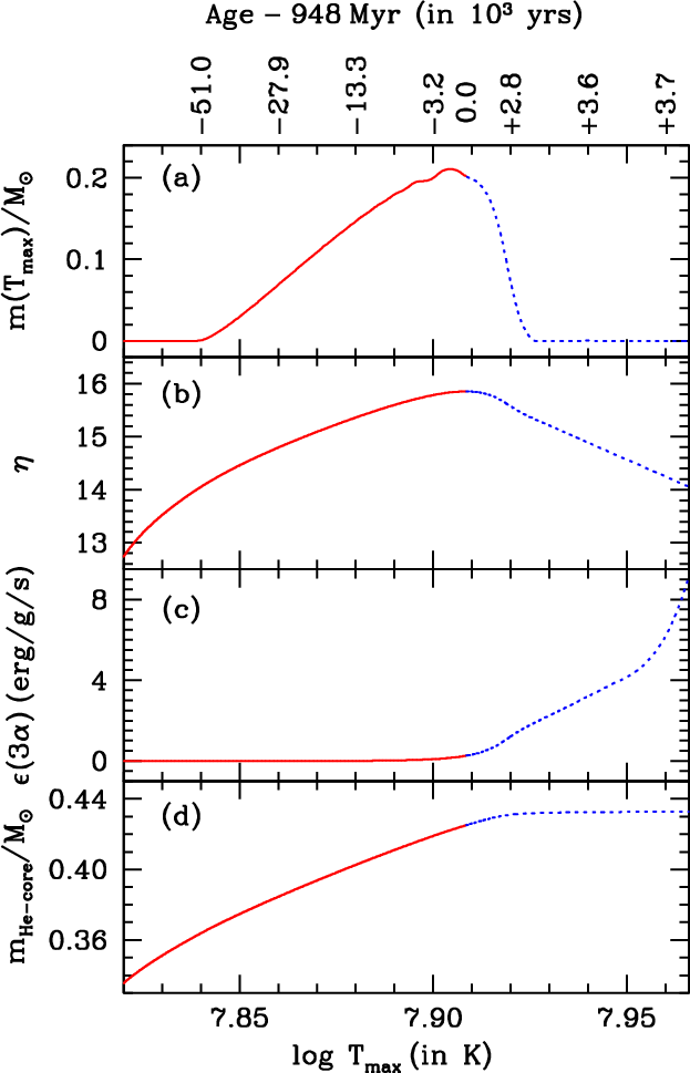 |
Figure 3:
The change, as a function of time ( upper x-axis), or equivalently as a function of maximum temperature in the star,
|
| Open with DEXTER | |
The actual age of the model on the helium-burning main sequence cannot,
of course, be assigned accurately because of the ``missing'' period of the
helium flash. However, the total duration of the helium flash phenomenon
and the subsequent stabilisation of the star on the helium-burning main
sequence is only ![]() 1.5 Myr (Piersanti et al. 2004), and hence the
uncertainty in the age in our helium-burning models is quite small.
1.5 Myr (Piersanti et al. 2004), and hence the
uncertainty in the age in our helium-burning models is quite small.
For slightly higher mass models (
![]() ), the evolution of
the star is followed continuously from the pre-main sequence stage till
the red clump stage. Since the helium ignition at the tip of the giant
branch occurs under non-degenerate conditions, there are no numerical
problems in such cases. The transition mass from violent to quiescent
helium ignition is a function of chemical composition. It has been
studied in detail by Sweigart et al. (1989). More recent illustration is found in
the tracks of Yi et al. (2003), which were constructed with a similar
version of YREC (Demarque et al. 2008).
), the evolution of
the star is followed continuously from the pre-main sequence stage till
the red clump stage. Since the helium ignition at the tip of the giant
branch occurs under non-degenerate conditions, there are no numerical
problems in such cases. The transition mass from violent to quiescent
helium ignition is a function of chemical composition. It has been
studied in detail by Sweigart et al. (1989). More recent illustration is found in
the tracks of Yi et al. (2003), which were constructed with a similar
version of YREC (Demarque et al. 2008).
There is an uncertainty in the age of the core helium-burning models because of the assumption of no mass loss on the red giant branch. Since the amount of mass lost in the giant phase is not known, the mass of the ZAHB model cannot be assigned accurately. Therefore, the ages of helium-burning models given in Tables 1 and 4 are, in fact, upper limits to the real ages.
2.5 Timescales of evolution
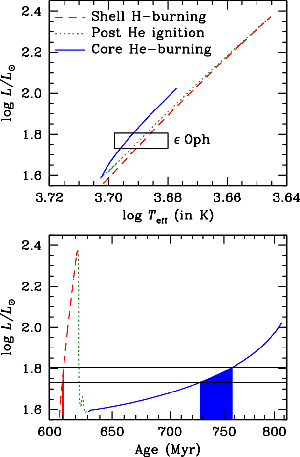 |
Figure 4:
The different timescales of the stellar evolutionary tracks in each crossing of the
|
| Open with DEXTER | |
A star of a given mass might cross the
![]() errorbox on the HR diagram three times - once upwards during shell H-burning, once downwards during the stabilisation of the star just after He ignition, and once again upwards during the phase of stable core He-burning. The timescales of evolution in these three phases are quite different, and consequently
the time spent inside the
errorbox on the HR diagram three times - once upwards during shell H-burning, once downwards during the stabilisation of the star just after He ignition, and once again upwards during the phase of stable core He-burning. The timescales of evolution in these three phases are quite different, and consequently
the time spent inside the
![]() box differs vastly.
Figure 4 illustrates the timescales of evolution in each crossing of the box for a 2.3
box differs vastly.
Figure 4 illustrates the timescales of evolution in each crossing of the box for a 2.3
![]() star. During the shell H-burning phase, it spends nearly 1.09 Myr inside the box. After He ignition in the core, it spends only 0.17 Myr during the rapid settling towards the He-burning main sequence, and finally it spends 30.59 Myr during the stable core He-burning phase. Similar timescales are found for other stars in this mass range. The time spent during the shell H-burning phase is typically
star. During the shell H-burning phase, it spends nearly 1.09 Myr inside the box. After He ignition in the core, it spends only 0.17 Myr during the rapid settling towards the He-burning main sequence, and finally it spends 30.59 Myr during the stable core He-burning phase. Similar timescales are found for other stars in this mass range. The time spent during the shell H-burning phase is typically ![]() 20 times shorter than that during
the core He-burning phase. Thus the probabilities of
20 times shorter than that during
the core He-burning phase. Thus the probabilities of
![]() being in the corresponding phases of evolution are in the same ratio.
being in the corresponding phases of evolution are in the same ratio.
3 Comparison of theoretical and observed frequencies
The theoretical frequencies of the stellar models were compared with the MOST data on
![]() .
Typically, in asteroseismic modelling studies, the comparison between a stellar model and the observed frequency data is carried out in terms of frequency separations, especially the large frequency separations, rather than the frequencies themselves. This is done to eliminate the uncertainty in the theoretical absolute
frequencies due to inadequate modelling of the stellar surface layers. However, this is possible only in the happy circumstance of detection of
a series of frequencies of the same degree and successive radial orders,
for which the large separations can be determined. For
.
Typically, in asteroseismic modelling studies, the comparison between a stellar model and the observed frequency data is carried out in terms of frequency separations, especially the large frequency separations, rather than the frequencies themselves. This is done to eliminate the uncertainty in the theoretical absolute
frequencies due to inadequate modelling of the stellar surface layers. However, this is possible only in the happy circumstance of detection of
a series of frequencies of the same degree and successive radial orders,
for which the large separations can be determined. For
![]() ,
Barban et al. (2007) indeed provide the frequencies of 9 successive radial
order modes. Thus it is possible to match the observed large
separations with the theoretical values from the models. However, as an
additional comparison, we also match the absolute frequencies of radial
modes of our stellar models with the MOST data.
,
Barban et al. (2007) indeed provide the frequencies of 9 successive radial
order modes. Thus it is possible to match the observed large
separations with the theoretical values from the models. However, as an
additional comparison, we also match the absolute frequencies of radial
modes of our stellar models with the MOST data.
Table 1:
Stellar parameters for the models with lowest
![]() and
and
![]() values in either shell H-burning or core He-burning phase.
values in either shell H-burning or core He-burning phase.
For each comparison, a reduced ![]() value is computed as
value is computed as
![\begin{displaymath}\ensuremath{\chi_\nu^2} = \frac{1}{N}\sum_{i=1}^N \left[\frac{\nu_{\rm MOST} -
\nu_{\rm model}}{\delta\nu_{\rm MOST}}\right]^2
\end{displaymath}](/articles/aa/full_html/2009/32/aa12351-09/img69.png) |
(1) |
![\begin{displaymath}\ensuremath{\chi_{\Delta\nu}^2} = \frac{1}{N-1}\sum_{i=2}^{N}...
... -
\Delta\nu_{\rm model}}{\delta\Delta\nu_{\rm MOST}}\right]^2
\end{displaymath}](/articles/aa/full_html/2009/32/aa12351-09/img70.png) |
(2) |
where
The best-fitting models in both shell H-burning and core He-burning
phases can reproduce the observed large separations fairly well. This is illustrated in Fig. 5. However, it turns out that the large separation corresponding to one of the observed modes at
![]() is nearly
is nearly ![]() away from the
theoretical value in all our models. This data point is always the
largest contributor to
away from the
theoretical value in all our models. This data point is always the
largest contributor to
![]() and
and
![]() .
We have ignored
this point while choosing our best model.
.
We have ignored
this point while choosing our best model.
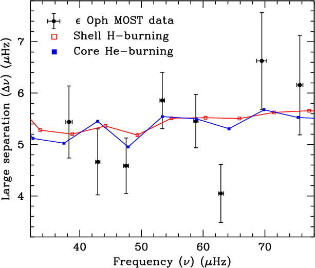 |
Figure 5:
The large frequency separations of best-fitting radial modes of stellar
models in the shell H-burning ( red open squares) and core
He-burning ( blue filled squares) phases inside the
|
| Open with DEXTER | |
The parameters of the models with the lowest
![]() and
and
![]() values are listed in Table 1. Notice that the
model with least
values are listed in Table 1. Notice that the
model with least
![]() in the shell H-burning phase has a
significantly high value of
in the shell H-burning phase has a
significantly high value of
![]() because of an overall shift in the
absolute frequencies. Given one criterion for comparison (either
because of an overall shift in the
absolute frequencies. Given one criterion for comparison (either
![]() or
or
![]() ), it is clear that the models in the shell
H-burning phase fit the data almost equally well as those in the core
He-burning phase. Thus, the present data is unable to distinguish
between these two phases of stellar evolution. However, as discussed in
Sect. 2.5, the likelihood of the star being in the core He-burning phase is greater than it being in the shell H-burning phase.
), it is clear that the models in the shell
H-burning phase fit the data almost equally well as those in the core
He-burning phase. Thus, the present data is unable to distinguish
between these two phases of stellar evolution. However, as discussed in
Sect. 2.5, the likelihood of the star being in the core He-burning phase is greater than it being in the shell H-burning phase.
Based on the best match between observed and model large separations,
the models indicate very similar parameters for both phases of
evolution. We estimate the stellar parameters from not only the models with lowest ![]() ,
but actually all models that have
,
but actually all models that have ![]() values
within 50% of the least
values
within 50% of the least ![]() .
The mass is estimated to be
.
The mass is estimated to be
![]() ,
while the metallicity of the best models are in the range of
,
while the metallicity of the best models are in the range of
![]() .
The radius lies in the range of
.
The radius lies in the range of
![]() .
The radius of
.
The radius of
![]() ,
however, can be measured
independently through interferometry, as described in the next section.
,
however, can be measured
independently through interferometry, as described in the next section.
4 Interferometric measurements
4.1 Instrumental setup
We observed
![]() in July 2006 at the CHARA Array
(ten Brummelaar 2005) using FLUOR, the Fiber Linked Unit for Optical
Recombination (Coudé du Foresto et al. 2003). This instrument is equipped with a near infrared K' band filter (
in July 2006 at the CHARA Array
(ten Brummelaar 2005) using FLUOR, the Fiber Linked Unit for Optical
Recombination (Coudé du Foresto et al. 2003). This instrument is equipped with a near infrared K' band filter (
![]() ).
We extracted the instrumental visibilities from the raw data using the
FLUOR data reduction software (Mérand 2006; Coudé du Foresto et al. 1997; Kervella et al. 2004). For
all the reported observations, we used the CHARA baselines S2-W2, with ground lengths of 177 m, which is mostly a north-south baseline in
orientation. The calibrator stars were chosen in the catalogue compiled
by Mérand et al. (2005), using criteria defined by these authors. They were
observed immediately before or after our targets in order to monitor the
interferometric transfer function of the instrument. These are listed in
Table 2 where the limb darkened angular diameter,
).
We extracted the instrumental visibilities from the raw data using the
FLUOR data reduction software (Mérand 2006; Coudé du Foresto et al. 1997; Kervella et al. 2004). For
all the reported observations, we used the CHARA baselines S2-W2, with ground lengths of 177 m, which is mostly a north-south baseline in
orientation. The calibrator stars were chosen in the catalogue compiled
by Mérand et al. (2005), using criteria defined by these authors. They were
observed immediately before or after our targets in order to monitor the
interferometric transfer function of the instrument. These are listed in
Table 2 where the limb darkened angular diameter,
![]() ,
and the angular separation,
,
and the angular separation, ![]() ,
with
,
with
![]() is given for each calibrator. For a more detailed description of the
observing procedure and the error propagation, the interested reader is
referred to Kervella et al. (2008) and Perrin (2003), respectively. The
resulting calibrated squared visibilities are listed in
Table 3, where B is the projected baseline length,
and ``PA'' is the azimuth of the projected baseline (counted positively
from North to East).
is given for each calibrator. For a more detailed description of the
observing procedure and the error propagation, the interested reader is
referred to Kervella et al. (2008) and Perrin (2003), respectively. The
resulting calibrated squared visibilities are listed in
Table 3, where B is the projected baseline length,
and ``PA'' is the azimuth of the projected baseline (counted positively
from North to East).
Table 2:
Calibrators used for
![]() .
.
Table 3:
Squared visibility measurements obtained for
![]() .
.
4.2 Angular diameter measurement and precision
In order to accurately measure
![]() angular diameters, we used many
known stellar calibrators and we repeated the observation on two
separate and consecutive nights. Since, in the end, the number of
visibility will always be small, statistically speaking, the final
confidence on the precision will rely more on the repeatability of the
the result and the consistency between the stellar calibrators.
angular diameters, we used many
known stellar calibrators and we repeated the observation on two
separate and consecutive nights. Since, in the end, the number of
visibility will always be small, statistically speaking, the final
confidence on the precision will rely more on the repeatability of the
the result and the consistency between the stellar calibrators.
Our observation strategy was designed to give maximum precision and confidence to our results. As a result, we achieve:
- the repeatability of the result. The first night gives
 mas, with a reduced
  of 0.9; the second night
 mas, with a reduced
of 0.3. This is consistent at the 0.01 mas level.
mas, with a reduced
of 0.3. This is consistent at the 0.01 mas level.
- the use of multiple slightly resolved calibrators of various
sizes. Indeed, if we assume we have an overall bias in the angular
diameter estimation of the calibrators, it is going to lead to a
differential calibrated visibility bias, depending on the size of the calibrator. For example, if we multiply the diameters of our calibrators by 1.05 (i.e. a 5% bias), the new diameter for
 is
is
 mas, with a reduced
of 2.5 instead of our result
mas, with a reduced
of 2.5 instead of our result
 mas, with a
reduced
of 1.0. Not only would our final result be barely
affected, but also the reduced
becomes much higher, because
points calibrated by our large calibrator become completely inconsistent with the rest of the batch.
mas, with a
reduced
of 1.0. Not only would our final result be barely
affected, but also the reduced
becomes much higher, because
points calibrated by our large calibrator become completely inconsistent with the rest of the batch.
4.3 Limb darkened angular diameter and photospheric radius
In order to estimate the unbiased angular diameter from the measured
visibilities it is necessary to know the intensity distribution of the light on the stellar disk, i.e., the limb darkening (LD). As we do not
fully resolve
![]() ,
we cannot measure the limb darkening directly
from the data. We thus model it using the MARCS models
(Gustafsson et al. 2008)
,
we cannot measure the limb darkening directly
from the data. We thus model it using the MARCS models
(Gustafsson et al. 2008)![]() for the computation of the intensity profile of the star, taking into account the actual spectral transmission function of the FLUOR instrument (Mérand 2005). The LD coefficients have been computed with the TURBOSPECTRUM code (Alvarez & Plez 1998). The result is shown in
Fig. 6. It is to be noted that taking an intensity profile from a different model, say the one predicted by the ATLAS9
model from Kurucz, using Claret's laws (Claret 2000), results in the same final result, within fractions of the statistical error bar. The
reason is that for the relatively large spectral bandwidth of FLUOR and considering that we measure first-lobe visibilities only, the difference between the MARCS and ATLAS models is negligible (of the order of a
fraction of our diameter error bar). The magnitude of the limb
darkening effect being much smaller in the infrared than in the visible, our resulting limb darkened angular diameter measurement in the K band is largely unaffected by the choice of the limb darkening model.
for the computation of the intensity profile of the star, taking into account the actual spectral transmission function of the FLUOR instrument (Mérand 2005). The LD coefficients have been computed with the TURBOSPECTRUM code (Alvarez & Plez 1998). The result is shown in
Fig. 6. It is to be noted that taking an intensity profile from a different model, say the one predicted by the ATLAS9
model from Kurucz, using Claret's laws (Claret 2000), results in the same final result, within fractions of the statistical error bar. The
reason is that for the relatively large spectral bandwidth of FLUOR and considering that we measure first-lobe visibilities only, the difference between the MARCS and ATLAS models is negligible (of the order of a
fraction of our diameter error bar). The magnitude of the limb
darkening effect being much smaller in the infrared than in the visible, our resulting limb darkened angular diameter measurement in the K band is largely unaffected by the choice of the limb darkening model.
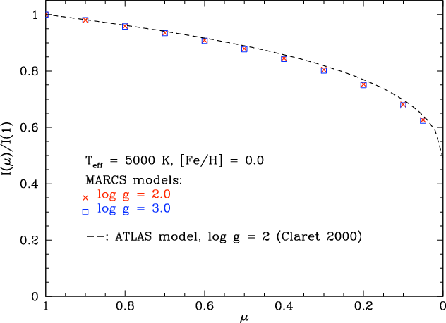 |
Figure 6:
Comparison of the intensity profiles of
|
| Open with DEXTER | |
The result of the visibility fit is presented in Fig. 7 using the MARCS limb darkening model. We derive the following limb darkened disk angular diameter:
| (3) |
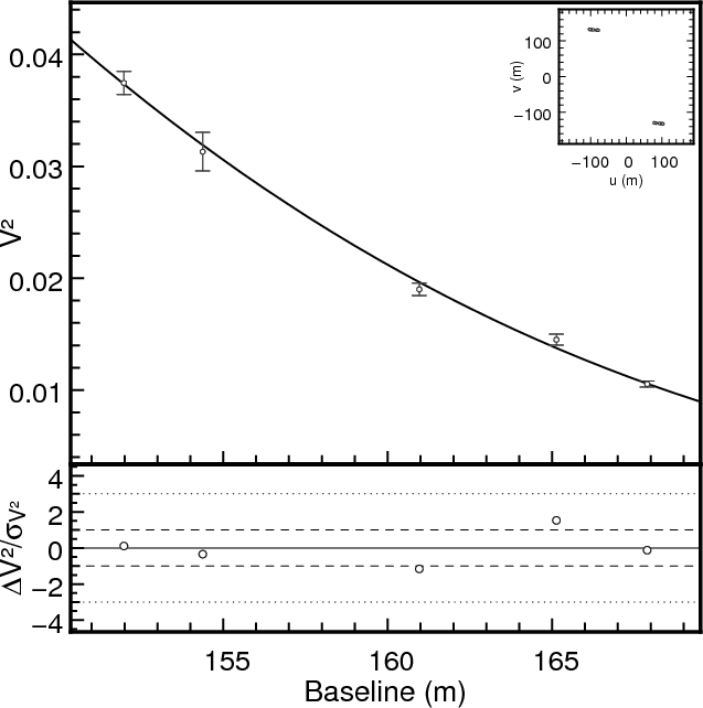 |
Figure 7:
Squared visibilities and adjusted limb darkened disk visibility model
for
|
| Open with DEXTER | |
| (4) |
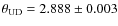
This value compares well with van Altena et al. (1995), and the original Hipparcos catalogue (ESA 1997), but is more precise. We finally derive the photospheric linear radius:
| (5) |
In spite of the the relatively high precision of the parallax, it is by far the limiting factor for the precision of the radius.
5 Discussion
In this study we have constructed stellar models of red giants in both shell H-burning and core He-burning phases and compared their adiabatic frequencies with the frequencies of
![]() observed by the MOST satellite and published by Barban et al. (2007). We have also measured the radius of the star through optical interferometry using the CHARA/FLUOR instrument.
observed by the MOST satellite and published by Barban et al. (2007). We have also measured the radius of the star through optical interferometry using the CHARA/FLUOR instrument.
We have demonstrated that the observed frequencies of
![]() are
consistent with radial p-mode pulsations of a red giant at the
relevant position on the HR diagram. Unfortunately, the radial mode
frequencies cannot distinguish between the two phases of stellar
evolution - shell H-burning and core He-burning. This is hardly
surprising, since the models inside the box on the HR diagram in either phase would have approximately similar radii, and the large separation depends crucially on the radius of the star. However, the seismic information helps us to constrain the radius of the star to a much narrower range than that possible by the errorbox on the HR diagram.
are
consistent with radial p-mode pulsations of a red giant at the
relevant position on the HR diagram. Unfortunately, the radial mode
frequencies cannot distinguish between the two phases of stellar
evolution - shell H-burning and core He-burning. This is hardly
surprising, since the models inside the box on the HR diagram in either phase would have approximately similar radii, and the large separation depends crucially on the radius of the star. However, the seismic information helps us to constrain the radius of the star to a much narrower range than that possible by the errorbox on the HR diagram.
Kallinger et al. (2008a) have carried out a seismic modelling study of
![]() also, but with important differences. Firstly, they have interpreted the observed peaks in the power spectrum of
also, but with important differences. Firstly, they have interpreted the observed peaks in the power spectrum of
![]() to be radial as well as nonradial modes. They identify the sharp narrow peaks in the power spectrum as long-lived nonradial modes, as compared to the broad Lorentzian envelopes, resulting in short-lived modes, which have been identified as radial modes by Barban et al. (2007). Secondly, they have
matched the observed frequency values, and not the large separations, to the theoretical model frequencies. Lastly, they have used only shell H-burning models. Given these differences, it is not surprising that they obtained a slightly different result than ours.
to be radial as well as nonradial modes. They identify the sharp narrow peaks in the power spectrum as long-lived nonradial modes, as compared to the broad Lorentzian envelopes, resulting in short-lived modes, which have been identified as radial modes by Barban et al. (2007). Secondly, they have
matched the observed frequency values, and not the large separations, to the theoretical model frequencies. Lastly, they have used only shell H-burning models. Given these differences, it is not surprising that they obtained a slightly different result than ours.
Little is known whether p-modes, radial or nonradial, can be excited in red giants to an amplitude high enough to be observable. A detailed theoretical study of models of ![]() UMa, observed by Buzasi et al. (2000) with the WIRE satellite, and of similar 2
UMa, observed by Buzasi et al. (2000) with the WIRE satellite, and of similar 2
![]() models on the lower giant branch, by Dziembowski et al. (2001) provides some insight on the oscillation characteristics of lower giant branch stars. Giant stars
are characterised by an inner cavity that can support gravity waves
(g-modes), and an outer cavity that supports acoustic waves
(p-modes). Observable modes in the outer cavity are mixed modes, with a g-mode character in the inner cavity and p-mode character in the
outer cavity. Dziembowski et al. (2001) showed that such mixed p-modes can have substantial amplitudes, and that low degree modes with
models on the lower giant branch, by Dziembowski et al. (2001) provides some insight on the oscillation characteristics of lower giant branch stars. Giant stars
are characterised by an inner cavity that can support gravity waves
(g-modes), and an outer cavity that supports acoustic waves
(p-modes). Observable modes in the outer cavity are mixed modes, with a g-mode character in the inner cavity and p-mode character in the
outer cavity. Dziembowski et al. (2001) showed that such mixed p-modes can have substantial amplitudes, and that low degree modes with ![]() ,
together with the radial p-modes can be unstable. According to their models of lower giant branch stars, high amplitudes in the outer cavity arise only for modes with
,
together with the radial p-modes can be unstable. According to their models of lower giant branch stars, high amplitudes in the outer cavity arise only for modes with ![]() .
The excitation properties of
p-modes in more luminous red giants lying around the middle of the red giant branch, which have very deep convection zones, such as
.
The excitation properties of
p-modes in more luminous red giants lying around the middle of the red giant branch, which have very deep convection zones, such as
![]() ,
are mostly unexplored.
,
are mostly unexplored.
A careful visual examination of the observed frequency spectrum of
![]() (Barban et al. 2007) reveals a clear comb-like structure with
reasonably regular spacing of
(Barban et al. 2007) reveals a clear comb-like structure with
reasonably regular spacing of ![]() 5.3
5.3
![]() .
In an adiabatic
pulsation calculation of a theoretical model, a series of regularly
spaced radial modes accompanied by a dense forest of nonradial modes are obtained (see Fig. 8). The observed frequencies of
.
In an adiabatic
pulsation calculation of a theoretical model, a series of regularly
spaced radial modes accompanied by a dense forest of nonradial modes are obtained (see Fig. 8). The observed frequencies of
![]() ,
as given by Barban et al. (2007), can be matched reasonably well to the radial modes. In principle, they can also be matched easily to many
of the closely spaced nonradial modes as well, but the question remains
as to why the majority of the nonradial modes are not observed.
,
as given by Barban et al. (2007), can be matched reasonably well to the radial modes. In principle, they can also be matched easily to many
of the closely spaced nonradial modes as well, but the question remains
as to why the majority of the nonradial modes are not observed.
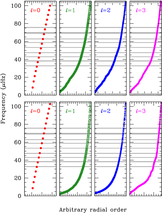 |
Figure 8:
Adiabatic pulsation frequencies of radial ( |
| Open with DEXTER | |
A possible explanation of this may be provided in terms of the
normalised mode inertia E, defined according to Christensen-Dalsgaard (2004) as
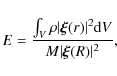 |
(6) |
where
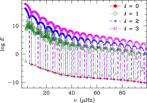 |
Figure 9:
Normalised mode inertia of
|
| Open with DEXTER | |
In a recent theoretical work involving nonadiabatic treatment of the
excitation mechanism, Dupret et al. (2009) have found that despite their low
amplitudes, a selection of nonradial modes may still have appreciable
heights in the power spectrum of red giants because of their long lifetimes,
and thus be detected in observations. However, the detection of such
modes depends crucially on the evolutionary stage of the star on the red
giant branch. Theoretical computations for intermediate red giant
branch stars like
![]() predict much longer lifetimes for nonradial modes (
predict much longer lifetimes for nonradial modes (![]() 50 days) than radial modes (
50 days) than radial modes (![]() 20 days) because of their larger inertia. But if the duration of observation is shorter than these lifetimes, as the case is for MOST observations of
20 days) because of their larger inertia. But if the duration of observation is shorter than these lifetimes, as the case is for MOST observations of
![]() ,
it is
not possible to resolve these nonradial modes in the power spectrum.
This implies that the modes attain smaller heights in the power spectrum
and they become extremely difficult to detect.
,
it is
not possible to resolve these nonradial modes in the power spectrum.
This implies that the modes attain smaller heights in the power spectrum
and they become extremely difficult to detect.
Further, in the higher part of the frequency domain, the detectable
nonradial modes also appear with an asymptotic regular separation
pattern similar to that found in main sequence stars. This means that the ![]() and
and ![]() modes will appear close to each other, with
the
modes will appear close to each other, with
the ![]() modes occurring roughly midway between them. For
modes occurring roughly midway between them. For
![]() such a pattern implies that if we consider nonradial modes to be present
in the spectrum, the large separation (of
such a pattern implies that if we consider nonradial modes to be present
in the spectrum, the large separation (of ![]() modes, for example)
would be almost double the value than that obtained by postulating only
radial modes. Such a high value of the large separation (
modes, for example)
would be almost double the value than that obtained by postulating only
radial modes. Such a high value of the large separation (
![]() )
is inconsistent with the position of
)
is inconsistent with the position of
![]() on the HR diagram. However, according to Dupret et al. (2009), the lifetimes of some
on the HR diagram. However, according to Dupret et al. (2009), the lifetimes of some ![]() modes which are strongly trapped in the envelope are comparable to that of the radial ones. So these envelope-trapped
modes which are strongly trapped in the envelope are comparable to that of the radial ones. So these envelope-trapped ![]() modes could indeed be detectable. Trapping of
modes could indeed be detectable. Trapping of ![]() modes is less efficient, as found by Dziembowski et al. (2001) too, and hence they may not be observable.
However, in the absence of any detailed calculations for the mode
amplitudes and lifetimes for the specific case of
modes is less efficient, as found by Dziembowski et al. (2001) too, and hence they may not be observable.
However, in the absence of any detailed calculations for the mode
amplitudes and lifetimes for the specific case of
![]() ,
in this work we have adopted Barban et al. (2007)'s interpretation of the frequencies as radial modes only. An alternative modelling analysis taking into account
the possibility of nonradial modes might lead to a different set of
model parameters, as found by Kallinger et al. (2008a), for example. The
theoretical justification behind the presence of only a few specific
nonradial modes among the possible dense spectrum of such modes requires
further detailed study.
,
in this work we have adopted Barban et al. (2007)'s interpretation of the frequencies as radial modes only. An alternative modelling analysis taking into account
the possibility of nonradial modes might lead to a different set of
model parameters, as found by Kallinger et al. (2008a), for example. The
theoretical justification behind the presence of only a few specific
nonradial modes among the possible dense spectrum of such modes requires
further detailed study.
Table 4:
Stellar parameters for the models with lowest
![]() and
and
![]() values in either shell H-burning or core He-burning phase that have radii within
values in either shell H-burning or core He-burning phase that have radii within
![]() of the interferometric radius.
of the interferometric radius.
Our interferometric measurements yield a value of the radius of
![]() that is in close agreement with the radii of our best models obtained
through seismic analysis. The interferometric radius was not used as a constraint to choose the best model, but was rather checked a posteriori against the seismic values. The range of possible values of radius of stellar models within the errorbox on the HR diagram for
that is in close agreement with the radii of our best models obtained
through seismic analysis. The interferometric radius was not used as a constraint to choose the best model, but was rather checked a posteriori against the seismic values. The range of possible values of radius of stellar models within the errorbox on the HR diagram for
![]() is
is
![]() to
to
![]() .
But the seismic information, specifically the
frequencies or the large separation, restricts the radius to a much
narrower range. The best-fitting models using large separation comparison have radii of
.
But the seismic information, specifically the
frequencies or the large separation, restricts the radius to a much
narrower range. The best-fitting models using large separation comparison have radii of
![]() for both shell H-burning and core
He-burning phases. This value is within
for both shell H-burning and core
He-burning phases. This value is within ![]() of the interferometric
radius. Even considering all models with
of the interferometric
radius. Even considering all models with
![]() constrains the range of radius to
constrains the range of radius to
![]() for frequency
comparison, and to
for frequency
comparison, and to
![]() for large separation comparison (see Fig. 10). This range encompasses the much
narrower limit for the radius set by the interferometric measurements.
It is remarkable that despite the inherent uncertainties in the
modelling of the outer layers of a star, the seismic analysis alone
leads to a value of the radius that is in such good agreement with an independent direct estimate of the radius. The radius obtained by Kallinger et al. (2008a) through frequency fitting,
for large separation comparison (see Fig. 10). This range encompasses the much
narrower limit for the radius set by the interferometric measurements.
It is remarkable that despite the inherent uncertainties in the
modelling of the outer layers of a star, the seismic analysis alone
leads to a value of the radius that is in such good agreement with an independent direct estimate of the radius. The radius obtained by Kallinger et al. (2008a) through frequency fitting,
![]() ,
seems to be more removed from the interferometric radius than our seismic value is,
although it is difficult to directly compare the two in view of the
absence of error bars for the former.
,
seems to be more removed from the interferometric radius than our seismic value is,
although it is difficult to directly compare the two in view of the
absence of error bars for the former.
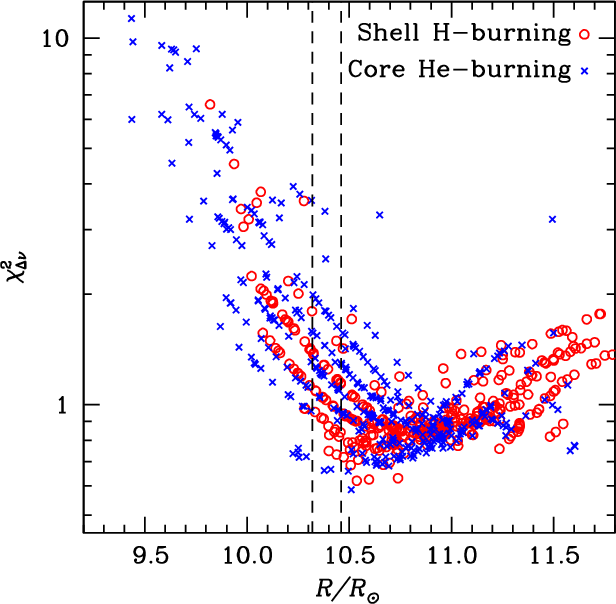 |
Figure 10:
The
|
| Open with DEXTER | |
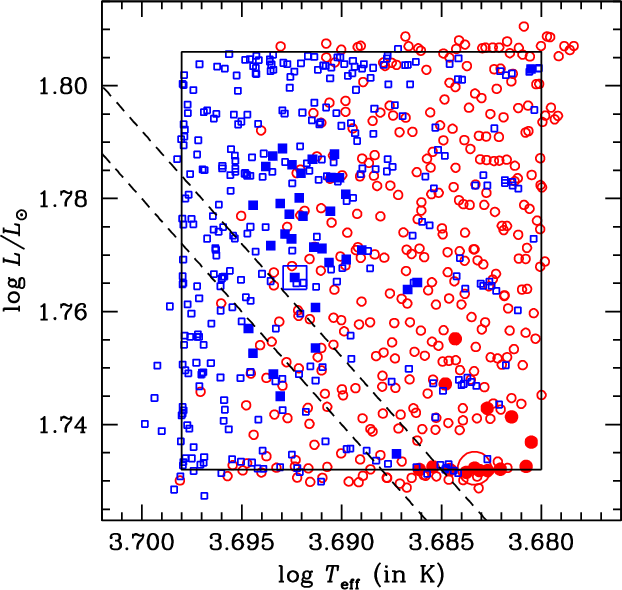 |
Figure 11:
All the computed stellar models inside and around the
|
| Open with DEXTER | |
As mentioned above, in the present study the independent estimate of the radius was not used as an additional constraint for choosing the best seismic model. However, since the modelling is in no way influenced by the presence of the radius information, we can check what would be the
result if indeed the radius is used as a constraint. We use the
![]() interval of the radius to restrict the position of the star on
the HR diagram, along with the adopted values of luminosity and effective
temperature. This leads to a trapezoidal area on the HR diagram (see
Fig. 11) as the errorbox for
interval of the radius to restrict the position of the star on
the HR diagram, along with the adopted values of luminosity and effective
temperature. This leads to a trapezoidal area on the HR diagram (see
Fig. 11) as the errorbox for
![]() .
The parameters of
the models inside this smaller errorbox that fit the seismic data best
are shown in Table 4. In this case, the minimisations
according to frequencies and large separations yield the same best
models in either phase of evolution. The minimum values of
.
The parameters of
the models inside this smaller errorbox that fit the seismic data best
are shown in Table 4. In this case, the minimisations
according to frequencies and large separations yield the same best
models in either phase of evolution. The minimum values of
![]() are marginally higher than in the more general case (cf. Table 1). However, the minimum
are marginally higher than in the more general case (cf. Table 1). However, the minimum
![]() values are
significantly higher, indicating that although the observed large
separations are quite well matched by these models, the absolute
frequency values are somewhat shifted. This is wholly expected since the
large separations are strongly influenced by the radius, even if the
frequencies themselves may be shifted because of inadequate modelling of the
surface effects. In other words, restricting the radius value implies a
strong constraint on the large separation, but not necessarily on the
absolute frequencies. This is also borne out in the more general case (when the radius constraint is not used) in Fig. 11 where the models with lowest
values are
significantly higher, indicating that although the observed large
separations are quite well matched by these models, the absolute
frequency values are somewhat shifted. This is wholly expected since the
large separations are strongly influenced by the radius, even if the
frequencies themselves may be shifted because of inadequate modelling of the
surface effects. In other words, restricting the radius value implies a
strong constraint on the large separation, but not necessarily on the
absolute frequencies. This is also borne out in the more general case (when the radius constraint is not used) in Fig. 11 where the models with lowest
![]() values (
values (![]() 0.8) in either
phase of evolution lie in a broad band almost parallel to the
interferometric radius band, indicating a constant higher radius value (
0.8) in either
phase of evolution lie in a broad band almost parallel to the
interferometric radius band, indicating a constant higher radius value (
![]() )
common to all of them. The seismic values of the mass and radius of
)
common to all of them. The seismic values of the mass and radius of
![]() yield an average large separation value of
yield an average large separation value of
![]() according to the scaling formula of Kjeldsen & Bedding (1995), which is completely consistent with the current data (Barban et al. 2007).
according to the scaling formula of Kjeldsen & Bedding (1995), which is completely consistent with the current data (Barban et al. 2007).
It is also possible to determine the effective temperature of the star from its measured radius and photometric data. From
Fig. 11 itself, it is evident that the intersection of the luminosity limits and the interferometric radius ranges indicates a temperature range of
![]() (
(
![]() K) which is consistent with our adopted range of effective temperature and has a similar uncertainty. Further, a fit of the available photometric data on
K) which is consistent with our adopted range of effective temperature and has a similar uncertainty. Further, a fit of the available photometric data on
![]() (BVJHK bands) using tabulated Kurucz models yields
(BVJHK bands) using tabulated Kurucz models yields
![]() (
(
![]() K) for surface gravity values typical of stars in the relevant zone of the HR diagram. Actually, a change of 0.1 dex in
K) for surface gravity values typical of stars in the relevant zone of the HR diagram. Actually, a change of 0.1 dex in ![]() makes a difference of only 1 K in
makes a difference of only 1 K in
![]() ,
while the uncertainty in the measured angular diameter contributes about 4 K
in the error estimate. Again, these value of
,
while the uncertainty in the measured angular diameter contributes about 4 K
in the error estimate. Again, these value of
![]() are completely
contained in the range that we have used from de Ridder et al. (2006). Thus our adopted values of L and
are completely
contained in the range that we have used from de Ridder et al. (2006). Thus our adopted values of L and
![]() are consistent with the independent measurements of parallax (Hipparcos) and the angular diameter (this paper).
are consistent with the independent measurements of parallax (Hipparcos) and the angular diameter (this paper).
It is evident from this study that the seismic information alone can go a long way in constraining the most important stellar parameters of red giants. Even with a very limited data set, it was possible to obtain a
reasonably narrow range of parameters for
![]() ,
and the radius
estimate from the seismic modelling stands in close agreement with a
completely independent interferometric measurement. However, the
accuracy of the models can be greatly enhanced by the additional
information about the interferometric radius. An independent radius
measurement, with a high precision such as provided by interferometry,
helps in reducing the size of the errorbox on the HR diagram, making the task of searching for the best model easier. This is the first instance of the coming together of asteroseismology and interferometry for red giant stars, and clearly illustrates the huge potential of this combination in detailed studies of such stars.
,
and the radius
estimate from the seismic modelling stands in close agreement with a
completely independent interferometric measurement. However, the
accuracy of the models can be greatly enhanced by the additional
information about the interferometric radius. An independent radius
measurement, with a high precision such as provided by interferometry,
helps in reducing the size of the errorbox on the HR diagram, making the task of searching for the best model easier. This is the first instance of the coming together of asteroseismology and interferometry for red giant stars, and clearly illustrates the huge potential of this combination in detailed studies of such stars.
Acknowledgements
The authors would like to thank all the CHARA Array and Mount Wilson Observatory day-time and night-time staff for their support. The CHARA Array was constructed with funding from Georgia State University, the National Science Foundation, the W. M. Keck Foundation, and the David and Lucile Packard Foundation. The CHARA Array is operated by Georgia State University with support from the College of Arts and Sciences, from the Research Program Enhancement Fund administered by the Vice President for Research, and from the National Science Foundation under NSF Grant AST 0606958. This work also received the support of PHASE, the high angular resolution partnership between ONERA, Observatoire de Paris, CNRS and University Denis Diderot Paris 7. This research took advantage of the SIMBAD and VIZIER databases at the CDS, Strasbourg (France), and NASA's Astrophysics Data System Bibliographic Services. Part of this work was supported by the Research Fund of K. U. Leuven under grant GOA/2003/04 for AM and CB. S.T.R. acknowledges partial support by NASA grant NNH09AK731. The authors thank Marc-Antoine Dupret and Sarbani Basu for their valuable comments and suggestions.
References
- Alvarez, R., & Plez, B. 1998, A&A, 330, 1109 [NASA ADS] (In the text)
- Bahcall, J. N., & Pinsonneault, M. H. 1992, Rev. Mod. Phys., 64, 885 [NASA ADS] [CrossRef] (In the text)
- Barban, C., Matthews, J. M., de Ridder, J., et al. 2007, A&A, 468, 1033 [NASA ADS] [CrossRef] [EDP Sciences]
- Böhm-Vitense, E. 1958, ZAp, 46, 108 [NASA ADS] (In the text)
- Buzasi, D., Catanzarite, J., Laher, R., et al. 2000, ApJ, 532, L133 [NASA ADS] [CrossRef] (In the text)
- Cayrel de Strobel, G., Soubiran, C., & Ralite, N. 2001, A&A, 373, 159 [NASA ADS] [CrossRef] [EDP Sciences]
- Christensen-Dalsgaard, J. 2004, Sol. Phys., 220, 137 [NASA ADS] [CrossRef] (In the text)
- Claret, A. 2000, A&A, 363, 1081 [NASA ADS] (In the text)
- Clayton, D. D. 1968, Principles of Stellar Evolution and Nucleosynthesis (New York: McGraw-Hill) (In the text)
- Cohen, M., Walker, R. G., Carter, B., et al. 1999, AJ, 117, 1864 [NASA ADS] [CrossRef] (In the text)
- Cole, P. W., & Deupree, R. G. 1983, ApJ, 269, 676 [NASA ADS] [CrossRef] (In the text)
- Coudé du Foresto, V., Ridgway, S., & Mariotti, J.-M. 1997, A&AS, 121, 379 [NASA ADS] [CrossRef] [EDP Sciences]
- Coudé du Foresto, V., Bordé, P., Mérand, A., et al. 2003, Proc. SPIE, 4838, 280 [NASA ADS] (In the text)
- Creevey, O. L., Monteiro, M. J. P. F. G., Metcalfe, T. S., et al. 2007, A&A, 659, 616 [NASA ADS] (In the text)
- Cunha M. S., Aerts, C., Christensen-Dalsgaard, J., et al. 2007, A&A Rev., 14, 217 [NASA ADS] (In the text)
- de Ridder, J., Barban, C., Carrier, F., et al. 2006, A&A, 448, 689 [NASA ADS] [CrossRef] [EDP Sciences]
- Demarque, P., & Mengel, J. G. 1971, ApJ, 164, 317 [NASA ADS] [CrossRef] (In the text)
- Demarque, P., Woo, J.-H., Kim, Y.-C., et al. 2004, ApJS, 155, 667 [NASA ADS] [CrossRef] (In the text)
- Demarque, P., Guenther, D. B., Li, L. H., Mazumdar, A., & Straka, C. W. 2008, Ap&SS, 316, 31 [NASA ADS] [CrossRef] (In the text)
- Dupret, M.-A., Belkacem, K., Samadi, R., et al. 2009, A&A, accepted (In the text)
- Dziembowski, W. A., Gough, D. O., Houdek, G., & Sienkiewicz, R. 2001, MNRAS, 328, 601 [NASA ADS] [CrossRef] (In the text)
- ESA 1997, The Hipparcos and Tycho Catalogues, ESA SP-1200 (In the text)
- Ferguson, J. W., Alexander, D. R., Allard, F., et al. 2005, ApJ, 623, 585 [NASA ADS] [CrossRef] (In the text)
- Frandsen, S., Carrier, F., Aerts, C., et al. 2002, A&A, 394, L5 [NASA ADS] [CrossRef] [EDP Sciences]
- Grevesse, N., & Sauval, A. J. 1998, Space Sci. Rev., 85, 161 [NASA ADS] [CrossRef] (In the text)
- Guenther, D. B. 1994, ApJ, 422, 400 [NASA ADS] [CrossRef] (In the text)
- Guenther, D. B., Demarque, P., Kim, Y.-C., & Pinsonneault, M. H. 1992, ApJ, 87, 372 [NASA ADS] [CrossRef] (In the text)
- Gustafsson, B., Edvardsson, B., Eriksson, K., et al. 2008, A&A, 486, 951 [NASA ADS] [CrossRef] [EDP Sciences] (In the text)
- Hekker, S., Barban, C., & Kallinger, T. 2008, Commun. Asteroseismol., 157, 319 [NASA ADS]
- Iglesias, C. A., & Rogers, F. J. 1996, ApJ, 464, 943 [NASA ADS] [CrossRef] (In the text)
- Itoh, N., Adachi, T., Nakagawa, M., Kohyama, Y., & Munakata, H. 1989, ApJ, 339, 354 [NASA ADS] [CrossRef] (In the text)
- Kallinger, T., Guenther, D. B., Matthews, J. M., et al. 2008a, A&A, 478, 497 [NASA ADS] [CrossRef] [EDP Sciences] (In the text)
- Kallinger, T., Guenther, D. B., Weiss, W. W., et al. 2008b, Commun. Asteroseismol., 153, 84 [NASA ADS] [CrossRef]
- Kervella, P., Ségransan, D., & Coudé du Foresto, V. 2004, A&A, 425, 1161 [NASA ADS] [CrossRef] [EDP Sciences]
- Kervella, P., Mérand, A., Pichon, B., et al. 2008, A&A, 488, 667 [NASA ADS] [CrossRef] [EDP Sciences] (In the text)
- Kjeldsen, H., & Bedding, T. R. 1995, A&A, 293, 87 [NASA ADS] (In the text)
- Lee, Y.-W., & Demarque, P. 1990, ApJS, 73, 709 [NASA ADS] [CrossRef]
- Mérand, A., Ph. D. Thesis 2005, Université Paris 7 (In the text)
- Mérand, A., Bordé, P., & Coudé du Foresto, V. 2005, A&A, 433, 1155 [NASA ADS] [CrossRef] [EDP Sciences] (In the text)
- Mérand, A., Coudé du Foresto, V., Kellerer, A., et al. 2006, Proc. SPIE, 6268, 46 [NASA ADS]
- Mocàk, M., Müller, E., Weiss, A., & Kiforidis, K. 2009, A&A, 501, 659 [NASA ADS] [CrossRef] [EDP Sciences] (In the text)
- Perrin, G. 2003, A&A, 400, 1173 [NASA ADS] [CrossRef] [EDP Sciences] (In the text)
- Piersanti, L., Tornambé, A., & Castellani, V. 2004, MNRAS, 353, 243 [NASA ADS] [CrossRef] (In the text)
- Reimers, D. 1977, A&A, 57, 395 [NASA ADS] (In the text)
- Rogers, F. J., & Nayfonov, A. 2002, ApJ, 576, 1064 [NASA ADS] [CrossRef] (In the text)
- Schwarzschild, M., & Härm, R. 1962, ApJ, 136, 158 [NASA ADS] [CrossRef] (In the text)
- Straka, C. W., Demarque, P., & Robinson, F. J. 2007, IAU Symp., 239, 388 [NASA ADS] (In the text)
- Sweigart, A. V. 1987, ApJS, 65, 95 [NASA ADS] [CrossRef]
- Sweigart, A. V., Greggio, L., & Renzini, A. 1989, ApJS, 69, 911 [NASA ADS] [CrossRef] (In the text)
- ten Brummelaar, T. A., McAlister, H. A., Ridgway, S. T., et al. 2005, ApJ, 628, 453 [NASA ADS] [CrossRef] (In the text)
- van Altena, W. F., Lee, J. T., & Hoffleit, E. D. 1995, The General Catalogue of Trigonometric Stellar Parallaxes, 4th Edn, Yale University Observatory (In the text)
- van Leeuwen, F. 2007a, Hipparcos, the New Reduction of the Raw Data, Astrophys. Space Sci. Libr., 350 (Springer)
- van Leeuwen, F. 2007b, A&A, 474, 653 [NASA ADS] [CrossRef] [EDP Sciences]
- Walker, G., Matthews, J., Kuschnig, R., et al. 2003, PASP, 115, 1023 [NASA ADS] [CrossRef] (In the text)
- Yi, S. K., Kim, Y.-C., & Demarque, P. 2003, ApJS, 144, 259 [NASA ADS] [CrossRef] (In the text)
Footnotes
All Tables
Table 1:
Stellar parameters for the models with lowest
![]() and
and
![]() values in either shell H-burning or core He-burning phase.
values in either shell H-burning or core He-burning phase.
Table 2:
Calibrators used for
![]() .
.
Table 3:
Squared visibility measurements obtained for
![]() .
.
Table 4:
Stellar parameters for the models with lowest
![]() and
and
![]() values in either shell H-burning or core He-burning phase that have radii within
values in either shell H-burning or core He-burning phase that have radii within
![]() of the interferometric radius.
of the interferometric radius.
All Figures
| |
Figure 1:
Stellar evolutionary tracks from the ZAMS to the shell H-burning RGB are shown with respect to the position of
|
| Open with DEXTER | |
| In the text | |
| |
Figure 2:
Stellar evolutionary tracks from the ZAHB to the end of He-burning main sequence are shown with respect to the position of
|
| Open with DEXTER | |
| In the text | |
| |
Figure 3:
The change, as a function of time ( upper x-axis), or equivalently as a function of maximum temperature in the star,
|
| Open with DEXTER | |
| In the text | |
| |
Figure 4:
The different timescales of the stellar evolutionary tracks in each crossing of the
|
| Open with DEXTER | |
| In the text | |
| |
Figure 5:
The large frequency separations of best-fitting radial modes of stellar
models in the shell H-burning ( red open squares) and core
He-burning ( blue filled squares) phases inside the
|
| Open with DEXTER | |
| In the text | |
| |
Figure 6:
Comparison of the intensity profiles of
|
| Open with DEXTER | |
| In the text | |
| |
Figure 7:
Squared visibilities and adjusted limb darkened disk visibility model
for
|
| Open with DEXTER | |
| In the text | |
| |
Figure 8:
Adiabatic pulsation frequencies of radial ( |
| Open with DEXTER | |
| In the text | |
| |
Figure 9:
Normalised mode inertia of
|
| Open with DEXTER | |
| In the text | |
| |
Figure 10:
The
|
| Open with DEXTER | |
| In the text | |
| |
Figure 11:
All the computed stellar models inside and around the
|
| Open with DEXTER | |
| In the text | |
Copyright ESO 2009
Current usage metrics show cumulative count of Article Views (full-text article views including HTML views, PDF and ePub downloads, according to the available data) and Abstracts Views on Vision4Press platform.
Data correspond to usage on the plateform after 2015. The current usage metrics is available 48-96 hours after online publication and is updated daily on week days.
Initial download of the metrics may take a while.