| Issue |
A&A
Volume 503, Number 2, August IV 2009
|
|
|---|---|---|
| Page(s) | 409 - 435 | |
| Section | Extragalactic astronomy | |
| DOI | https://doi.org/10.1051/0004-6361/200912240 | |
| Published online | 27 May 2009 | |
The Westerbork SINGS survey
II Polarization, Faraday rotation, and magnetic fields
G. Heald1 - R. Braun2 - R. Edmonds3
1 - Netherlands Institute for Radio Astronomy (ASTRON), Postbus 2, 7990 AA Dwingeloo, The Netherlands
2 - CSIRO-ATNF, PO Box 76, Epping, NSW 1710, Australia
3 - New Mexico State University, Department of Astronomy, PO Box 30001, MSC 4500, Las Cruces, New Mexico, 88003-8001, USA
Received 1 April 2009 / Accepted 20 May 2009
Abstract
A sample of large northern Spitzer Infrared Nearby Galaxies Survey (SINGS) galaxies has recently been observed with the
Westerbork Synthesis Radio Telescope (WSRT). We present observations of the linearly polarized radio continuum emission in this WSRT-SINGS galaxy sample. Of the 28 galaxies treated in this paper, 21 are detected in polarized radio continuum at 18- and 22-cm wavelengths. We utilize the rotation measure synthesis
(RM-Synthesis) method, as implemented by Brentjens & de Bruyn (2005, A&A, 441, 1217), to
coherently detect polarized emission from a large fractional
bandwidth, while simultaneously assessing the degree of Faraday
rotation experienced by the radiation along each line-of-sight. This
represents the first time that the polarized emission and its
Faraday rotation have been systematically probed down to
![]() 10
10 ![]() Jy beam-1 RMs for a large sample of
galaxies. Non-zero Faraday rotation is found to be ubiquitous in all
of the target fields, from both the Galactic foreground and the
target galaxies themselves. In this paper, we present an overview of
the polarized emission detected in each of the WSRT-SINGS
galaxies. The most prominent trend is a systematic modulation of the
polarized intensity with galactic azimuth, such that a global
minimum in the polarized intensity is seen toward the kinematically
receding major axis. The implied large-scale magnetic field geometry
is discussed in a companion paper. A second novel result is the
detection of multiple nuclear Faraday depth components that are
offset to both positive and negative RM by
Jy beam-1 RMs for a large sample of
galaxies. Non-zero Faraday rotation is found to be ubiquitous in all
of the target fields, from both the Galactic foreground and the
target galaxies themselves. In this paper, we present an overview of
the polarized emission detected in each of the WSRT-SINGS
galaxies. The most prominent trend is a systematic modulation of the
polarized intensity with galactic azimuth, such that a global
minimum in the polarized intensity is seen toward the kinematically
receding major axis. The implied large-scale magnetic field geometry
is discussed in a companion paper. A second novel result is the
detection of multiple nuclear Faraday depth components that are
offset to both positive and negative RM by
![]() in all
targets that host polarized (circum-)nuclear emission.
in all
targets that host polarized (circum-)nuclear emission.
Key words: ISM: magnetic fields - galaxies: magnetic fields - radio continuum: galaxies
1 Introduction
In the study of star formation properties and evolution of galaxies, an important ingredient is the magnetic field content of the ISM. Yet the precise role that magnetic fields play in regulating star formation, and the role of magnetic fields in the evolution of galaxy disks, is still far from well understood. One reason for this gap is that a systematic survey of magnetic field content in galaxies over a range of Hubble type and star formation properties had, until recently, not been performed.
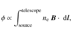
Magnetic fields are expected to play an important role in several aspects of star formation and galaxy evolution. First, magnetic fields are a crucial consideration in the energy balance of the ISM (e.g., Beck 2007), and in particular are likely important in determining the conditions for gravitational instability that lead to the inital stages of star formation (McKee & Ostriker 2007). Magnetic fields are expected to be important agents in helping to shape galactic evolution on large scales (Boulares & Cox 1990), while the longevity of familiar morphological features such as spiral arm ``spurs'' may be dependent on the presence of ordered magnetic fields (Shetty & Ostriker 2006). Finally, magnetic fields may be an important piece of the puzzle in understanding how the disk-halo interaction proceeds (e.g., Tüllmann et al. 2000), and thus in determining how matter and energy are redistributed throughout a galactic disk and indeed within galaxy groups and clusters by feedback processes.
Clearly, magnetic fields should be a major consideration in the study of star formation and galaxy evolution. However, observational measurements of the magnetic fields in nearby galaxies are relatively few. A review of the available observations is not warranted here, but some of the most recent studies, obtained with widely varying observational setups, include those of: NGC 6946 (Beck 2007); NGC 5194 (Berkhuijsen et al. 1997); NGC 4254 (Chyzy et al. 2007); and the Large Magellanic Cloud (Gaensler et al. 2005). Taken together, all of the observations indicate a tendency for magnetic fields to be oriented in spiral patterns in disk galaxies, even in galaxies with no spiral structure visible in the gaseous or stellar morphology (e.g. NGC 4414; Soida et al. 2002). Where spiral arms are visible, the fields tend to be more ordered in the interarm regions. Halos seem to have large-scale magnetic fields; the ordered fields typically lie parallel to the disk in edge-on galaxies, and then turn to a more perpendicular orientation as distance from the midplane increases.
Table 1: Summary of survey galaxies.
Information about the magnetic fields in galaxies is most efficiently
obtained using two complementary techniques. The nonthermal
synchtrotron emission generated by relativistic electrons spiraling in
a magnetic field oriented perpendicular to the line of sight (LOS) is
linearly polarized. The electric field vector of the polarized
radiation is oriented perpendicular to the magnetic field that
accelerates the source electrons, and the radiation itself is beamed
parallel to the trajectory of the ultra-relativistic electron. Thus,
the plane of polarization of the observed synchrotron radiation is
directly related to the component of the magnetic field perpendicular
to the LOS (![]() )
in the observed object. Moreover, the
synchrotron emissivity is proportional to the product of
)
in the observed object. Moreover, the
synchrotron emissivity is proportional to the product of
![]() and the relativistic electron density nCR,
where
and the relativistic electron density nCR,
where ![]() is the spectral index (e.g., Longair 1994).
This makes the observed
polarized intensity itself a good tracer of
is the spectral index (e.g., Longair 1994).
This makes the observed
polarized intensity itself a good tracer of ![]() .
This
straightforward correspondence is complemented by the second technique
for measuring magnetic fields: Faraday rotation. This effect is
produced when polarized radiation passes through a magnetized plasma,
which is birefringent (Gardner & Whiteoak 1963). The intrinsic
linear polarization angles of the radiation are rotated by a different
angle depending on the wavelength of the radiation. The effect is
characterized by the Faraday ``rotation measure''. The value of the
rotation measure (RM) is dependent on the electron density
.
This
straightforward correspondence is complemented by the second technique
for measuring magnetic fields: Faraday rotation. This effect is
produced when polarized radiation passes through a magnetized plasma,
which is birefringent (Gardner & Whiteoak 1963). The intrinsic
linear polarization angles of the radiation are rotated by a different
angle depending on the wavelength of the radiation. The effect is
characterized by the Faraday ``rotation measure''. The value of the
rotation measure (RM) is dependent on the electron density ![]() in the magnetized plasma, and the component of the magnetic field along
the LOS (
in the magnetized plasma, and the component of the magnetic field along
the LOS (
![]() ). The sign of RM is determined by whether
). The sign of RM is determined by whether
![]() points toward or away from the observer.
See Sect. 2.2 for an in-depth discussion.
points toward or away from the observer.
See Sect. 2.2 for an in-depth discussion.
The Spitzer Infrared Nearby Galaxies Survey (SINGS; Kennicutt et al. 2003) was conceived as a multi-wavelength Legacy program intended to address the question of how stars form in a wide range of galactic ISM environments. The strength of such a concerted survey campaign is that it draws together data over the widest possible range of observing bands to provide as much information as possible about the physical conditions in the galaxy ISM being investigated. Gaps in the coverage are generally covered by supplementary surveys such as The H I Nearby Galaxy Survey (THINGS; Walter et al. 2008).
One such supplementary survey is the Westerbork SINGS survey (WSRT-SINGS; Braun et al. 2007), which provides 18- and 22-cm radio continuum data, in all four Stokes parameters, for a subset of the SINGS galaxies (the survey selection criteria are discussed below). Together with the SINGS survey itself, the data provided by the WSRT supplement enable, for example, investigation into the origin of the FIR-radio correlation (Murphy et al. 2006). In this paper and a companion work (Braun et al. 2009; hereafter Paper III), we utilize the linear polarization products of the WSRT-SINGS data to investigate the magnetic field content of the ISM in the subsample galaxies.
Of the galaxies that make up the SINGS sample, not all are observable
with the WSRT. Because the individual antennas are arranged in a
linear east-west array, the synthesized beam is significantly extended
in the north-south direction when observing objects at low
declination. At the frequencies observed in this survey, the
synthesized beam would be ![]() 1
1
![]() for sources at
for sources at
![]() ;
we therefore exclude galaxies below this
declination limit. Furthermore, in order to ensure that the galaxies
themselves are large enough on the sky that they are spatially
resolved, the additional criterion was adopted that the optical B band
diameter at a surface brightness of 25 mag arcsec-2,
;
we therefore exclude galaxies below this
declination limit. Furthermore, in order to ensure that the galaxies
themselves are large enough on the sky that they are spatially
resolved, the additional criterion was adopted that the optical B band
diameter at a surface brightness of 25 mag arcsec-2,
![]() .
With the addition of four galaxies in the
Starburst sample of Rieke, a total of 34 galaxies were observed in the WSRT-SINGS program. Twenty-eight of those galaxies are studied here; their properties are summarized in Table 1.
The columns are: (1) Galaxy ID; (2) RC3 Hubble type; (3) D25;
(4) Inclination; (5) Spiral pitch angle (from Kennicutt (1981));
(6) Spiral sense (+1 for counter-clockwise, -1 for
clockwise); (7) Kinematic PA (measured east of north) of the receding major axis; (8) Reference for inclination and PA values;
(9) Synthesized beam ellipticity (a/b, where the minor axis of the beam is in all cases
.
With the addition of four galaxies in the
Starburst sample of Rieke, a total of 34 galaxies were observed in the WSRT-SINGS program. Twenty-eight of those galaxies are studied here; their properties are summarized in Table 1.
The columns are: (1) Galaxy ID; (2) RC3 Hubble type; (3) D25;
(4) Inclination; (5) Spiral pitch angle (from Kennicutt (1981));
(6) Spiral sense (+1 for counter-clockwise, -1 for
clockwise); (7) Kinematic PA (measured east of north) of the receding major axis; (8) Reference for inclination and PA values;
(9) Synthesized beam ellipticity (a/b, where the minor axis of the beam is in all cases
![]() ,
and the beam position angle is
,
and the beam position angle is
![]() ;
(10) Noise levels in P; (11) Integrated flux in P with an estimated error; (12) Estimated foreground RM that applies to the target field; (13) Integrated 1365 MHz flux in I (from Braun et al. 2007).
;
(10) Noise levels in P; (11) Integrated flux in P with an estimated error; (12) Estimated foreground RM that applies to the target field; (13) Integrated 1365 MHz flux in I (from Braun et al. 2007).
This paper is organized as follows. We describe the observations and data reduction steps in Sect. 2, with a particular emphasis on describing the RM-Synthesis method (Sect. 2.2), which is a critical component of the analysis utilized in this work. An overview of the polarized emission detected in each of the survey galaxies is presented in Sect. 3. For those galaxies with detected polarized emission, a discussion of some derivable characteristics is given in Sect. 4. Properties of the global magnetic field geometries revealed by these observations are treated in detail in Paper III. A more detailed study of individual galaxies will form the basis of forthcoming work. We conclude the paper in Sect. 5 and provide an outlook for future investigations.
2 Observations and data reduction
2.1 Data collection and ``standard'' data reduction
The observational parameters of the WSRT-SINGS survey were presented in detail by Braun et al. (2007), and we list the most relevant points here. Each galaxy was observed for at least 12 h in two bands covering the ranges 1300-1432 and 1631-1763 MHz (22- and 18-cm, respectively). The observing band was switched every 5 mn during an individual synthesis. In each band, the correlator was set up to provide 512 channels separated by 312.5 kHz. Eight 20-MHz subbands (64 channels each) were used at each observing frequency, and the central subband frequencies were arranged to be separated by 16 MHz. This setup allows us to disregard frequency channels suffering from bandpass rolloff (which affects each of the individual subbands), and maximizes the continuity of the frequency coverage while still providing a large total bandwidth. Data were obtained in all four Stokes parameters.
The basic data reduction steps of each 20 MHz subband are also discussed by Braun et al. (2007); we repeat the most relevant details here. After careful editing of incidental radio frequency interference (RFI) the bandpass calibration in amplitude and phase was determined using the calibration sources 3C147, 3C286, CTD93 and 3C138 within the AIPS package (Greisen 2003). Relative broadband gains in the two perpendicular linear polarizations (X and Y) were then determined, after modifications to several key tasks (SETJY and CALIB) to enable the representation of source models, and the calculation of gain solutions, with arbitrary values of the Stokes parameters (I,Q,U,V). This was necessary to permit an equivalent representation of the measured linear polarization products (with an unchanging parallactic angle) within a software package that normally assumes right- and left-handed circular polarization products. Basic polarization calibration was then accomplished by determining the cross-polarization leakage from 3C147, under the assumption that this source is intrinsically unpolarized. The phase offset of the X and Y polarizations (which is assumed to remain constant during each 12 h track) was then determined using the linearly polarized emission properties of either 3C286 [e.g. (I,Q,U,V) =(14.65,0.56,1.26,0.00) Jy near 1400 MHz] or 3C138. In cases where both 3C286 and 3C138 were observed bracketing the 12 h target track, it was possible to determine the consistency of the phase offset, which was found to be constant to better than 1-2 degrees. After a final check that the correct Stokes parameters were recovered for all calibration sources (both polarized and unpolarized), the calibrated data were exported from the AIPS package. Further refinement of the polarization calibration was accomplished via self-calibration of each 20 MHz subband within the Miriad package (Sault et al. 1995) using the detected emission in each target field in Stokes I, Q and U. This step corrects for time-variable instrumental or ionospheric phase errors.
Following these reduction steps, the Q and U maps in each narrowband frequency channel (of 312.5 kHz) were imaged individually. They were
CLEANed within mask regions derived from smoothed versions of
the total Stokes I map in each subband. The same restoring beam size was used at all channel frequencies; see Table 1 for the effective resolution in each galaxy. Primary
beam corrections were applied to each channel map individually. The primary
beam correction was performed using the standard WSRT model [the
primary beam response is approximated with the function
![]() ,
where c=68 at L-band frequencies,
,
where c=68 at L-band frequencies, ![]() is the
frequency in GHz, and r is the distance from the pointing center in
radians]. An improved primary beam correction for the WSRT has been
developed by Popping & Braun (2008) but is little different from
the standard treatment at the small field angles which are considered
here. After primary beam correction, the channel maps were arranged
into cubes, and analyzed with the RM-Synthesis technique (described in
Sect. 2.2). Individual channel maps are used
as input to the RM-Synthesis software because the technique can be thought of
as a technique for determining the Faraday rotation measure which maximizes the
polarized signal-to-noise ratio across the full frequency band.
is the
frequency in GHz, and r is the distance from the pointing center in
radians]. An improved primary beam correction for the WSRT has been
developed by Popping & Braun (2008) but is little different from
the standard treatment at the small field angles which are considered
here. After primary beam correction, the channel maps were arranged
into cubes, and analyzed with the RM-Synthesis technique (described in
Sect. 2.2). Individual channel maps are used
as input to the RM-Synthesis software because the technique can be thought of
as a technique for determining the Faraday rotation measure which maximizes the
polarized signal-to-noise ratio across the full frequency band.
Stokes V images were generated, and the intensity histograms in those images are Gaussian, with an rms of about
![]() .
In some fields, very bright continuum sources far from the field center have
instrumental circular polarization, at the
.
In some fields, very bright continuum sources far from the field center have
instrumental circular polarization, at the
![]() level.
level.
2.2 RM synthesis
As discussed above, the effect of Faraday rotation is to change the
intrinsic polarization angle of the radiation (![]() )
by an amount
depending on the wavelength of the radiation. More specifically, the
observed polarization angles after Faraday rotation are
)
by an amount
depending on the wavelength of the radiation. More specifically, the
observed polarization angles after Faraday rotation are

where
where
Equation (1) is valid only in physical situations where
all of the polarized emission is observed at a single Faraday depth
![]() .
In more complicated circumstances
(for instance, emission that
arises both beyond and between two distinct Faraday rotating clouds
along the LOS; for an in-depth discussion see Sokoloff et al. 1998),
the simple relation is no longer valid. By expressing
the polarization vector as an exponential (
.
In more complicated circumstances
(for instance, emission that
arises both beyond and between two distinct Faraday rotating clouds
along the LOS; for an in-depth discussion see Sokoloff et al. 1998),
the simple relation is no longer valid. By expressing
the polarization vector as an exponential (
![]() ), using
Eq. (1) for
), using
Eq. (1) for ![]() ,
and integrating over all
Faraday depths, Burn (1966) shows that
,
and integrating over all
Faraday depths, Burn (1966) shows that
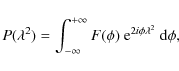
where
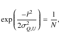
Under the assumption that ![]() is constant for all
is constant for all ![]() ,
the
Fourier transform-like Eq. (3) can be inverted to give an expression for the Faraday dispersion function:
,
the
Fourier transform-like Eq. (3) can be inverted to give an expression for the Faraday dispersion function:
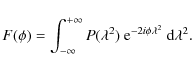
Everything on the right-hand side of Eq. (4) is observable. However, we only measure discrete (positive) values of
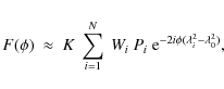
where Wi are weights which are allowed to differ from unity, and the normalization factor K is the inverse of the discrete sum over Wi. Note that the term
and is conceptually equivalent to the dirty beam encountered when performing image synthesis with an array of radio telescopes. Just as a radio interferometer discretely samples uv-space, here we discretely sample
Previous rotation measure experiments have had to rely on relatively few
measurements in frequency space. But with modern correlator backends
like the one at the WSRT, the technique of determining ![]() as
shown in Eq. (5) is made possible. The
practical aspects of this technique have been developed by
Brentjens & de Bruyn (2005). We use software developed by
Brentjens to perform the inversion shown in
Eq. (5) and obtain a reconstruction of
as
shown in Eq. (5) is made possible. The
practical aspects of this technique have been developed by
Brentjens & de Bruyn (2005). We use software developed by
Brentjens to perform the inversion shown in
Eq. (5) and obtain a reconstruction of
![]() .
The software takes cubes of Stokes Q and U images
in single frequency channels as input, along with a specification of the
frequency at each plane of the cubes. As
output, cubes of Stokes Q and U in planes of constant
.
The software takes cubes of Stokes Q and U images
in single frequency channels as input, along with a specification of the
frequency at each plane of the cubes. As
output, cubes of Stokes Q and U in planes of constant ![]() are
obtained. Simply put, the inversion amounts to the computation of the
implied values of Q and U for a whole series of trial values of the
Faraday depth,
are
obtained. Simply put, the inversion amounts to the computation of the
implied values of Q and U for a whole series of trial values of the
Faraday depth, ![]() .
In this way, the coherent sensitivity of the
entire observing band to polarized emission is retained, irrespective
of possible Faraday rotation within the band, as long as such rotation is well resolved by the
.
In this way, the coherent sensitivity of the
entire observing band to polarized emission is retained, irrespective
of possible Faraday rotation within the band, as long as such rotation is well resolved by the ![]() sampling.
sampling.
The polarization vectors described by the values of Q and U in each plane can be thought of as having been corrected for Faraday rotation - but note that the vectors have been derotated to a common non-zero value of ![]() ,
namely to
,
namely to
![]() ,
as shown
in Eq. (5). Hence, to obtain the intrinsic polarization angle at each value of
,
as shown
in Eq. (5). Hence, to obtain the intrinsic polarization angle at each value of ![]() ,
multiplication of our
reconstructed
,
multiplication of our
reconstructed
![]() by
by
![]() must be performed. Further explanation
regarding this detail is provided in Appendix A.
must be performed. Further explanation
regarding this detail is provided in Appendix A.
The frequency sampling provided by the WSRT-SINGS survey gives
sensitivity to polarized emission up to a maximum Faraday depth of
![]() (see Brentjens & de Bruyn 2005), where
(see Brentjens & de Bruyn 2005), where
![]() refers
to the channel separation. A search for large rotation measure
emission was performed for each of the galaxy fields, by performing
RM-Synthesis on the observed Q and U cubes in the range
refers
to the channel separation. A search for large rotation measure
emission was performed for each of the galaxy fields, by performing
RM-Synthesis on the observed Q and U cubes in the range
![]() (albeit with coarse
(albeit with coarse ![]() sampling). No emission at high values of Faraday depth was found in
any of the target fields. Next, RM-Synthesis was performed on the 22 cm
data alone, from
sampling). No emission at high values of Faraday depth was found in
any of the target fields. Next, RM-Synthesis was performed on the 22 cm
data alone, from
![]() to
to
![]() with fine sampling
(
with fine sampling
(
![]() ). Given the
). Given the ![]() width of the 22 cm band, the
width of the 22 cm band, the
![]() resolution element (FWHM) is
resolution element (FWHM) is
![]() .
The first sidelobe of the RMSF is at 24% of the main lobe. The sidelobe level can be reduced, at the expense of lower
.
The first sidelobe of the RMSF is at 24% of the main lobe. The sidelobe level can be reduced, at the expense of lower ![]() resolution, by tapering in
resolution, by tapering in ![]() space (by allowing Wi to deviate from unity in Eq. (5), and as illustrated in Fig. 1). After tapering with a Gaussian with
space (by allowing Wi to deviate from unity in Eq. (5), and as illustrated in Fig. 1). After tapering with a Gaussian with
![]() ,
the width of the main lobe is
,
the width of the main lobe is
![]() ,
and the first sidelobe is reduced to 2% of the RMSF peak. Increasing the denominator in the tapering function serves to further decrease the sidelobe level, while increasing the width of the main lobe. After testing a series of different tapers, this particular choice was selected as a reasonable tradeoff between sidelobe height and RMSF width. The cubes produced in this way can be used as a (very) low resolution verification of complicated
,
and the first sidelobe is reduced to 2% of the RMSF peak. Increasing the denominator in the tapering function serves to further decrease the sidelobe level, while increasing the width of the main lobe. After testing a series of different tapers, this particular choice was selected as a reasonable tradeoff between sidelobe height and RMSF width. The cubes produced in this way can be used as a (very) low resolution verification of complicated ![]() spectra.
spectra.
RM-Synthesis was also performed on the combination of the 18 cm and
22 cm data. The results of this operation were used for most of the
subsequent analysis. Together, the two bands provide a ![]() resolution of
resolution of
![]() .
This is comparable to the maximum Faraday depth to which about 50% sensitivity to the polarized intensity is retained of about
.
This is comparable to the maximum Faraday depth to which about 50% sensitivity to the polarized intensity is retained of about
![]() .
However, due to the large gap in frequency coverage between the two bands, the RMSF has large sidelobes, as shown in Fig. 1. The first sidelobes are at about the 78% level in P, which can potentially cause serious confusion, particularly in cases where polarized emission is detected at multiple
.
However, due to the large gap in frequency coverage between the two bands, the RMSF has large sidelobes, as shown in Fig. 1. The first sidelobes are at about the 78% level in P, which can potentially cause serious confusion, particularly in cases where polarized emission is detected at multiple ![]() along a single LOS. This difficulty can be alleviated by using a deconvolution technique similar to the Högbom CLEAN algorithm (Sect. 2.3).
along a single LOS. This difficulty can be alleviated by using a deconvolution technique similar to the Högbom CLEAN algorithm (Sect. 2.3).
2.3 Faraday dispersion function deconvolution
Once the RM-Synthesis was performed for each field, the ![]() spectra were deconvolved using a variation of the Högbom CLEAN, as outlined by Brentjens (2007). The deconvolution is
complex-valued and operates along the
spectra were deconvolved using a variation of the Högbom CLEAN, as outlined by Brentjens (2007). The deconvolution is
complex-valued and operates along the ![]() dimension, which is the
third axis of the
dimension, which is the
third axis of the ![]() and
and ![]() cubes produced by the
RM-Synthesis technique. The steps of the procedure, called RM-CLEAN, are described in detail in Appendix A. Briefly, one iteratively subtracts scaled
versions of the RMSF from the reconstructed Faraday dispersion function
until the noise floor is reached, after which a smoothed
representation of the ``CLEAN model'' is used as the approximate
true Faraday dispersion function. In this paper, we take the RM-CLEAN cutoff to be equal to the noise in the individual
cubes produced by the
RM-Synthesis technique. The steps of the procedure, called RM-CLEAN, are described in detail in Appendix A. Briefly, one iteratively subtracts scaled
versions of the RMSF from the reconstructed Faraday dispersion function
until the noise floor is reached, after which a smoothed
representation of the ``CLEAN model'' is used as the approximate
true Faraday dispersion function. In this paper, we take the RM-CLEAN cutoff to be equal to the noise in the individual
![]() and
and ![]() maps, and the gain factor is 0.1 (see Appendix A for a more extensive description of these parameters).
maps, and the gain factor is 0.1 (see Appendix A for a more extensive description of these parameters).
Examples of the result of running RM-CLEAN on dirty ![]() spectra are shown in Figs. 2 and 3. In Fig. 2, a single-valued
spectra are shown in Figs. 2 and 3. In Fig. 2, a single-valued
![]() spectrum has been RM-CLEANed. The only benefit is that
the sidelobe structure has been significantly reduced. Note that
the deconvolution routine is unable to improve the
spectrum has been RM-CLEANed. The only benefit is that
the sidelobe structure has been significantly reduced. Note that
the deconvolution routine is unable to improve the ![]() resolution,
which is determined by the spread of sampled frequencies. In the
right-hand panels, the data are compared to the
resolution,
which is determined by the spread of sampled frequencies. In the
right-hand panels, the data are compared to the ![]() representation of the RM-CLEAN components found during the
procedure. A solution equivalent to the best linear fit to
representation of the RM-CLEAN components found during the
procedure. A solution equivalent to the best linear fit to
![]() -vs-
-vs-![]() has been determined. That this type of
deconvolution is mathematically identical to a least-squares fit in
the inverse Fourier domain has been shown by Schwarz (1978). In Fig. 3, a more complicated
has been determined. That this type of
deconvolution is mathematically identical to a least-squares fit in
the inverse Fourier domain has been shown by Schwarz (1978). In Fig. 3, a more complicated ![]() is
shown. Note that in cases such as this, where multiple structures are detected, the location of the peak of the fainter component is shifted relative to its true position because of confusion with sidelobes from the brighter component. Particularly in such cases, deconvolution is required to recover source parameters.
is
shown. Note that in cases such as this, where multiple structures are detected, the location of the peak of the fainter component is shifted relative to its true position because of confusion with sidelobes from the brighter component. Particularly in such cases, deconvolution is required to recover source parameters.
Final on-axis sensitivities in the deconvolved ![]() cubes are listed in Table 1 for each galaxy. In view of the combined frequency coverage contributing to P (1300-1432 and
1631-1763 MHz), the effective center frequency is about 1530 MHz.
cubes are listed in Table 1 for each galaxy. In view of the combined frequency coverage contributing to P (1300-1432 and
1631-1763 MHz), the effective center frequency is about 1530 MHz.
2.4 Analysis of deconvolved Faraday depth cubes
The spatial distribution of polarized emission was determined by
selecting the peak in each
![]() spectrum. The grayscale maps of these images are shown in Fig. 4, with overlaid
contours of the 22 cm Stokes-I maps for comparison. Since polarized
intensity has Ricean, rather than Gaussian statistics
(see Wardle & Kronberg 1974), some care needs to be taken in
determining the integrated value of P. In the absence of source
signal, the noise has a Rayleigh distribution with a mean (the
``Ricean bias'') and variance of
spectrum. The grayscale maps of these images are shown in Fig. 4, with overlaid
contours of the 22 cm Stokes-I maps for comparison. Since polarized
intensity has Ricean, rather than Gaussian statistics
(see Wardle & Kronberg 1974), some care needs to be taken in
determining the integrated value of P. In the absence of source
signal, the noise has a Rayleigh distribution with a mean (the
``Ricean bias'') and variance of
 |
(7) |
and
 |
(8) |
for an rms noise in Q and U of
We have carefully determined the noise level and Ricean bias in
each target. To do this,
we have determined the mean and variance
in each image of peak P within a central, polygonal region (free of emission). The variances that we measure (and list in
Table 1) are in good agreement with the expectation noted above,
![]() ,
for a Rayleigh
distribution. However, the bias values that we measure are
in all cases enhanced by a factor of about two over the simple expectation,
,
for a Rayleigh
distribution. However, the bias values that we measure are
in all cases enhanced by a factor of about two over the simple expectation,
![]() .
The cause of this
high Ricean bias level is that the peak value of
.
The cause of this
high Ricean bias level is that the peak value of ![]() has been extracted from a cube covering Faraday depths
between -500 and
has been extracted from a cube covering Faraday depths
between -500 and
![]() with an effective resolution of about
with an effective resolution of about
![]() ,
and has thus been chosen from some 7 independent
samples. The Rayleigh distribution function is given by
,
and has thus been chosen from some 7 independent
samples. The Rayleigh distribution function is given by
 |
(9) |
where r represents the flux in a given sample. In a Faraday dispersion function which contains only noise (no signal), the expectation value for the largest (
 |
(10) |
or
![\begin{displaymath}{\hat r} = \sigma_{Q,U}[2~\ln(N)]^{0.5}.
\end{displaymath}](/articles/aa/full_html/2009/32/aa12240-09/img130.png) |
(11) |
This should be a good estimator of the Ricean bias in our maps. Since we have N=7, we obtain
For determination of the integrated P (or useful limits on P) for
each target (as listed in Table 1), we have not
carried out a spatial background subtraction of the noise floor, but
instead have simply blanked the images at a level of
3
![]() .
At these brightnesses, the Ricean
bias has already declined to below about 5%
(Wardle & Kronberg 1974), so that no further bias correction of
the integrated P was applied. The P emission was integrated within the smallest possible polygonal region which enclosed the region of significant target emission while excluding any apparent background sources. For comparison, we also list the integrated I of each target at 1365 MHz from Braun et al. (2007).
.
At these brightnesses, the Ricean
bias has already declined to below about 5%
(Wardle & Kronberg 1974), so that no further bias correction of
the integrated P was applied. The P emission was integrated within the smallest possible polygonal region which enclosed the region of significant target emission while excluding any apparent background sources. For comparison, we also list the integrated I of each target at 1365 MHz from Braun et al. (2007).
Polarized emission maps were also produced (using only the 22 cm data) for the purpose of determining the polarized fraction in these galaxies. The peak polarized intensity was extracted for each spatial pixel, and then divided by the corresponding 22 cm Stokes-I value. Clip levels were set at 4 times the noise level in both maps. Thus, polarization fraction estimates are not available for the faintest emission detected in the sample. The polarized fraction values are discussed in Sect. 3.2.
In order to determine the Faraday depth at the peak of the ![]() spectra, we fit a parabola to the top three points in the oversampled, RM-CLEANed
spectra, we fit a parabola to the top three points in the oversampled, RM-CLEANed ![]() spectra. The result is called
spectra. The result is called
![]() .
.
The polarization angle at the Faraday depth thus determined was obtained via
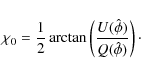 |
(12) |
We refer to this as the intrinsic polarization angle (
Errors associated with the magnetic field orientations were estimated by propagating errors through the mathematical operations required to calculate the quantity. Since
 |
(13) |
error propagation yields the uncertainty in our determination of the intrinsic polarization angle,
 |
(14) |
The quantity
 |
(15) |
where
Note that magnetic field orientations are easily interpreted only if
the deconvolved ![]() spectrum is single-valued. If there is more
than one
spectrum is single-valued. If there is more
than one ![]() component, then the magnetic field orientations
determined in this way only apply to the brightest component of
polarized emission. The deconvolved Faraday depth cubes
were analyzed to identify locations where multiple Faraday depths might be
present (Sect. 4.3).
These are noted throughout the paper, where appropriate.
component, then the magnetic field orientations
determined in this way only apply to the brightest component of
polarized emission. The deconvolved Faraday depth cubes
were analyzed to identify locations where multiple Faraday depths might be
present (Sect. 4.3).
These are noted throughout the paper, where appropriate.
3 Overview
Here, we summarize the main features of interest observed for each galaxy field based on a comparison of the polarized and total continuum brightness, together with the (Faraday rotation corrected) magnetic field orientation shown in Fig. 4, and the Faraday depth where peak polarized intensity is detected in Fig. 6.
3.1 Rotation measures of discrete background sources
In addition to the primary targets of our program, each observed field also contains a number of background sources with significant
polarized brightness. While many of these sources are unresolved at
the modest angular resolution of our study (![]() 15''), a significant
number are also resolved into the classical edge-brightened double
morphology associated with high luminosity radio galaxies
(e.g. Miley 1980). Lobe separations of 1-2 arcmin are
common, while a handful of objects with 5-10 arcmin angular size are
detected. We have determined the Faraday depth and the associated
error for the significantly detected polarized sources in the central
15''), a significant
number are also resolved into the classical edge-brightened double
morphology associated with high luminosity radio galaxies
(e.g. Miley 1980). Lobe separations of 1-2 arcmin are
common, while a handful of objects with 5-10 arcmin angular size are
detected. We have determined the Faraday depth and the associated
error for the significantly detected polarized sources in the central
![]() of our fields, making a particular note of the source
morphology and classifying sources as unresolved, double, triple
(double plus core), extended or complex. The individual lobes of
double radio sources were measured separately where practical. The
rotation measures listed in Table 2 were determined for each source from a plot of Faraday depth versus polarized brightness within a rectangular box that isolated the source (component). The listed RM is that of the peak in P while the error
corresponds to the HWHM of the distribution. The columns are:
(1) Galaxy field; (2) Discrete source position; (3) Morphology;
(4) Rotation measure with estimated error. Morphologies are classified
as unresolved: UNR, double: DBL, triple: TRPL, complex: CMPLX and
extended: EXT. For DBL and TRPL sources, the individual lobes
(N, S, E or W) are measured where possible, always begining with the
brightest one (in Stokes P). The weaker lobe is prefaced by its flux
ratio with respect to the brighter. When the source is (possibly)
affected by the target galaxy disk the morphology is further flagged
as FG(?).
of our fields, making a particular note of the source
morphology and classifying sources as unresolved, double, triple
(double plus core), extended or complex. The individual lobes of
double radio sources were measured separately where practical. The
rotation measures listed in Table 2 were determined for each source from a plot of Faraday depth versus polarized brightness within a rectangular box that isolated the source (component). The listed RM is that of the peak in P while the error
corresponds to the HWHM of the distribution. The columns are:
(1) Galaxy field; (2) Discrete source position; (3) Morphology;
(4) Rotation measure with estimated error. Morphologies are classified
as unresolved: UNR, double: DBL, triple: TRPL, complex: CMPLX and
extended: EXT. For DBL and TRPL sources, the individual lobes
(N, S, E or W) are measured where possible, always begining with the
brightest one (in Stokes P). The weaker lobe is prefaced by its flux
ratio with respect to the brighter. When the source is (possibly)
affected by the target galaxy disk the morphology is further flagged
as FG(?).
From the values in Table 2 it is apparent that when multiple, double-lobed sources are detected in an individual galaxy field then they generally have RMs that are in good agreement with one another. Unresolved sources in the field have RMs which are sometimes consistent, but seem to have a larger intrinsic scatter. Furthermore, when the lobes of double-lobed sources are within a factor of two in brightness they generally have better RM agreement, often as good as 1-2 rad m-2. For more extreme lobe brightness ratios, this consistency declines. To the extent that a single Galactic foreground RM contribution is appropriate in a particular field, the scatter in the measured RMs of the background sources is likely caused by variations in the intrinsic RMs of the sources themselves.
Since the likely red-shift of the luminous edge-brightened double sources we detect is greater than about z = 0.8 (Condon et al. 1998), the associated physical sizes are likely in the range 0.5-5 Mpc. The large physical separation of such radio lobes from the host galaxy makes it unlikely that high densities of thermal electrons will be mixed with the emitting regions. A relevant phenomenon which has been documented is the tendency for enhanced Faraday depolarization and RM fluctuations to be seen toward the fainter lobe of a pair (in both Stokes I and particularly P) (Garrington et al. 1988; Laing et al. 2006; Laing 1988). This phenomenon is consistent with the fainter lobe being the more distant one and its radiation suffering additional propagation effects while passing through the magneto-ionic halo of the host galaxy. A prediction of this interpretation is that edge-brightened doubles with equal brightness lobes are least likely to have differences in their associated Faraday depth, as we confirm. In any case, it is likely that well-separated lobes of luminous radio galaxies can provide a good estimate of the line-of-sight rotation measure with a minimal intrinsic contribution, in contrast to unresolved and possibly core-dominated AGN, for which a local host contribution to the Faraday depth is more likely.
A plausible method of estimating the Galactic foreground contribution
to the RM in each field seems to be a weighted median value
whereby double-lobed sources, particularly those of similar lobe
brightness, are given a very high weight. Some discussion of these
considerations is given below for each target field in turn, with the
result listed in Table 1. While the majority of our
target galaxies are well-removed from the Galactic plane
(
![]() ), where it is plausible that a single foreground RM
may be expected to apply to a region of
), where it is plausible that a single foreground RM
may be expected to apply to a region of
![]() ,
the two
exceptions are the fields containing NGC 7331 (
,
the two
exceptions are the fields containing NGC 7331 (
![]() )
and
NGC6946 (
)
and
NGC6946 (
![]() ). Diffuse, patchy polarized emission from the
Galaxy is apparent in these fields, accentuating the likelihood that
foreground RM fluctuations may also be present. We stress that we have
in no case made use of polarized emission from the target galaxy
itself to estimate the Galactic foreground RM, since this would bias
the outcome by artificially imposing a zero mean RM on the target
galaxy. For those targets in the direction of the Virgo cluster, or
more generally along the Super-galactic plane, there is also the
possibility that a non-zero contribution to the RM seen toward the
distant background radio galaxies of Table 2 arises within these media. Detection of such a contribution would require a much more extensive sampling of the RM sky, such as envisioned for the Square Kilometre Array and its Pathfinders
(e.g. Johnston et al. 2008).
). Diffuse, patchy polarized emission from the
Galaxy is apparent in these fields, accentuating the likelihood that
foreground RM fluctuations may also be present. We stress that we have
in no case made use of polarized emission from the target galaxy
itself to estimate the Galactic foreground RM, since this would bias
the outcome by artificially imposing a zero mean RM on the target
galaxy. For those targets in the direction of the Virgo cluster, or
more generally along the Super-galactic plane, there is also the
possibility that a non-zero contribution to the RM seen toward the
distant background radio galaxies of Table 2 arises within these media. Detection of such a contribution would require a much more extensive sampling of the RM sky, such as envisioned for the Square Kilometre Array and its Pathfinders
(e.g. Johnston et al. 2008).
3.2 Notes on individual galaxies
Here, we discuss the polarized features detected in each of the target
fields. For much of the analysis, we utilize the 18 + 22 cm (deconvolved)
Faraday cubes, and the associated peak P and
![]() maps shown in Figs. 4 and 6. Comparisons with optical images are shown in Fig. 5. We occasionally refer to the Faraday cubes produced using the 22 cm data alone. Trends in
the azimuthal and radial variations in polarized flux and Faraday RM lead to a generic, consistent picture of the global magnetic field geometry in the spiral galaxies included in our sample
(see Sect. 4.2). These trends and the global
magnetic field geometry are discussed in detail in Paper III. Most
galaxies with extended polarized flux show signs of broadened Faraday dispersion functions in small localized regions; see
Sect. 4.3 for details. All galaxies with compact (circum-)nuclear polarized emission show signs of significant Faraday structure in their nuclei. This is discussed in Sect. 4.4.
maps shown in Figs. 4 and 6. Comparisons with optical images are shown in Fig. 5. We occasionally refer to the Faraday cubes produced using the 22 cm data alone. Trends in
the azimuthal and radial variations in polarized flux and Faraday RM lead to a generic, consistent picture of the global magnetic field geometry in the spiral galaxies included in our sample
(see Sect. 4.2). These trends and the global
magnetic field geometry are discussed in detail in Paper III. Most
galaxies with extended polarized flux show signs of broadened Faraday dispersion functions in small localized regions; see
Sect. 4.3 for details. All galaxies with compact (circum-)nuclear polarized emission show signs of significant Faraday structure in their nuclei. This is discussed in Sect. 4.4.
Table 2: Discrete source rotation measures.
Holmberg II:
There is no convincingly detected polarized emission from Holmberg II. There is possibly very faint (at/below about the 4
IC 2574:
IC 2574 does not show evidence for significant polarized emission in either the 22 cm map or the 18 + 22 cm map. Since only unresolved polarized background sources are detected in this field, the Galactic foreground RM remains quite uncertain at about
NGC 628 (M74):
This relatively face-on spiral galaxy shows substantial polarized emission in the form of an incomplete ring near the edge of the optical disk which is brightest at PA
NGC 925:
There is no polarized emission detected in this galaxy. However, several faint background sources are seen toward the edges of the field. Excluding the unresolved polarized source most discrepant from the single double source lobe, we obtain an estimate of the Galactic foreground RM with a value of about
NGC 2403:
There is a faint polarized component which is predominantly diffuse, but is too faint to characterize well with the current observations. Smoothing to a beam size of
NGC 2841:
In Stokes I, Braun et al. (2007) note a diffuse ``hourglass'' structure, with the long axis of the hourglass oriented perpendicular to the disk major axis. In the polarized emission, the highest brightnesses are seen along the minor axis trailing away slowly to the northwest and more rapidly to the southeast. The lowest brightness of polarized emission occurs near the receding major axis (PA = 153
NGC 2903:
In this galaxy, one of the Starburst supplement to the basic SINGS sample, bright polarized arcs are detected along both sides of the minor axis trailing away in brightness slowly to the northeast and more rapidly to the southwest. The lowest brightness of polarized emission occurs on the receding major axis (PA = 204
NGC 2976:
There is very faint diffuse polarized emission associated with this galaxy, together with a modest enhancement along the southwestern edge of the optical disk. Only a single lobe of one double source is detected in this field, yielding a Galactic foreground RM of
NGC 3184:
In this galaxy, faint polarized emission is apparent over much of the northern half of the disk. The lowest brightness of polarized emission occurs near the receding major axis (PA = 179
NGC 3198:
No significant polarized emission is detected in this target, apart from a possible detection of the nucleus. An equal brightness double source in the field allows a very consistent assessment of the Galactic foreground RM of
NGC 3627 (M66):
Bright polarized emission is detected in this galaxy, with a conspicuous north-south gradient of the fractional polarization. It originates in both optical spiral arm and in interarm regions. The polarized fraction at 22 cm is less than 1% in the bright optical bar and inner disk of the galaxy, and increases in the regions outside of the spiral arms to as much as 15% on the eastern minor axis. The lowest brightness of polarized emission occurs near the receding major axis (PA = 173
NGC 3938:
Moderately faint polarized emission is detected in this almost face-on spiral. The polarized emission is concentrated to the outer disk and is enhanced in inter-arm regions. In contrast to other galaxies in our sample, the lowest brightness of polarized emission seem to occur near the approaching rather than the receding major axis (i.e., opposite to PA = 204
NGC 4125:
In this elliptical galaxy, Braun et al. (2007) report a continuum source at the nucleus, which we find is not polarized. They also report a double radio galaxy just to the southwest, the southern component of which is polarized at about the 5% level. The three double sources in this field provide a very consistent measurement of the Galactic foreground RM of
NGC 4236:
In this galaxy, Braun et al. (2007) report detecting continuum emission from the bright knots in the disk. There is no polarized counterpart associated with these features. The double background radio source behind the disk of NGC 4236 is detected in polarization, at about the 7% polarized fraction level with an RM of
NGC 4254 (M99):
Bright polarized emission is detected from an incomplete ring extending from PA
NGC 4321 (M100):
In this spiral galaxy, polarized emission is clearly detected throughout most of the disk. In the northwest, bright polarized emission is present throughout the interarm regions. But in the southeast the polarized surface brigntess declines dramatically. The lowest brightness of polarized emission occurs near the receding major axis (PA = 159
NGC 4450:
No significant polarized emission is detected in this galaxy. The almost equal double and brighter lobe of a triple in the field allow consistent assessment of the Galactic foreground RM of
NGC 4559:
In this spiral galaxy, diffuse continuum emission is detected, but the polarized component is extremely faint and only detected in a small region in the southeast portion of the disk. This asymmetry is again consistent with the lowest polarized intensity to be seen on the receding major axis. Deeper observations would be needed to better characterize the polarized emission. The equal double in the southern part of the field provides a consistent estimate of the Galactic foreground RM of
NGC 4569 (M90):
In this moderately inclined spiral galaxy, polarized emission is detected in the central disk region on either side of the minor axis. Polarized intensity declines more slowly to the southwest and more rapidly to the northeast (where the receding major axis is located (PA = 23
NGC 4631:
In this edge-on interacting spiral, the polarized emission is found in a roughly X-shaped morphology, and comes mainly from the extraplanar regions. The disk itself seems to be largely depolarized. Polarized emission is detected in the central region and in each of the four extraplanar galaxy quadrants. The north side is brighter in polarization than the south side. The brightest polarized intensity is from the northeast quadrant, which is the region where the dramatic HI extension studied by Rand (1994) is located. The polarized structure runs roughly parallel with the HI extension, but fills the region between the disk and the HI filament. The polarized fraction in this galaxy is less than one percent in the central regions and increases with height above the midplane. At the largest z-heights, the polarized fraction reaches as high as 30-40% in some places. The magnetic field lines run along the X-shaped polarized morphology. In the northeast quadrant, they run almost parallel to the HI extension, but these seem to be unrelated. The polarized structures reported here have been observed previously by Hummel et al. (1991) and Golla & Hummel (1994). The best estimate of the Galatic foreground RM in this direction comes from the unconfused double source in the field with an RM of
NGC 4725:
Extremely faint polarized emission is detected in this moderately inclined barred spiral galaxy, with the polarized emission originating at both ends of the minor axis. The polarized emission avoids the bar, which is at a position angle of about 45 degrees, and is mostly found on the outer periphery of the ring-like structure. The polarized emission is too faint to allow investigation of its detailed properties; deeper observations would be required. It is not possible to say anything about the magnetic field orientation, as too little signal is available. The foreground RM from the Galaxy in this direction can be estimated from the double radio source in the field at
NGC 4736 (M94):
The polarized emission in this galaxy is seen from both the inner
star-forming disk and also concentrated along the minor axis,
particularly in the form of a possible polarized lobe directed toward
the southwest. Within the central disk, the polarized intensity
declines to a minimum in the direction of the receding major axis
(PA = 296
NGC 4826 (M64):
There is a low level of polarized emission detected in the southern quadrant of this system that nowhere exceeds 4
NGC 5033:
The polarized emission in this galaxy is associated with the bright inner continuum disk reported by Braun et al. (2007). It has a roughly X-shaped appearance, which may be indicative of minor axis outflows, as seen elsewhere in our sample. The polarized brightness declines to a minimum in the direction of the receding major axis (PA = 352
NGC 5055 (M63):
Diffuse polarized emission is detected from the disk of this inclined galaxy on both sides of the minor axis. The highest brightnesses are associated with the zone of strong warping of the gaseous disk in the southwest at the edge of the star-forming disk. A fainter counterpart is seen in the northeast. The minimum in polarized intensity occurs at the PA of the receding major axis (PA = 102
NGC 5194
(M51):
In M51, the polarized emission is clearly detected throughout the
disk, though there are large variations in the polarized fraction. The
bright polarized emission traces out a spiral pattern that runs
parallel to the optical arms. The minimum in polarized intensity occurs
at the PA of the receding major axis (PA = 172
NGC 6946:
The polarized emission is strongly detected from the northeast half of this galaxy, tapering away toward the southwest. The minimum in polarized intensity occurs at the PA of the receding major axis (PA = 243
Unfortunately
only a single well-resolved double background source is detected in
this field (about
![]() southwest of NGC 6946), and this source is quite
asymmetric. The brighter lobe has a well-defined RM of
southwest of NGC 6946), and this source is quite
asymmetric. The brighter lobe has a well-defined RM of ![]() rad m-2. Several other sources in the field are possibly
influenced by RM contributions from the disk of NGC 6946 itself;
including the extended background source at
(
rad m-2. Several other sources in the field are possibly
influenced by RM contributions from the disk of NGC 6946 itself;
including the extended background source at
(![]() 20:35:19,
20:35:19, ![]() +60:02:05) just
+60:02:05) just
![]() south of the NGC 6946 disk that appears to be a barely resolved
(
south of the NGC 6946 disk that appears to be a barely resolved
(
![]() )
double with a well-defined RM of
)
double with a well-defined RM of ![]() rad m-2. As
previously noted, the low Galactic latitude of this field
(
rad m-2. As
previously noted, the low Galactic latitude of this field
(
![]() ,
decreasing to the southeast) enhances the likelihood
of fluctuations in the foreground RM. We suggest that the most likely
value of the foreground affecting NGC 6946 is an RM of
,
decreasing to the southeast) enhances the likelihood
of fluctuations in the foreground RM. We suggest that the most likely
value of the foreground affecting NGC 6946 is an RM of ![]() rad m-2, but stress that there is a substantial systematic
uncertainty in this value. Ehle & Beck (1993) and
Beck (2007) have previously determined a value of
rad m-2, but stress that there is a substantial systematic
uncertainty in this value. Ehle & Beck (1993) and
Beck (2007) have previously determined a value of
![]() in this field, which is consistent with the
mean Faraday depth that we have observed in the disk of NGC 6946
(see Fig. 6). We note that their foreground RM
value is derived using the diffuse emission of NGC 6946 itself, while
our derivation was performed using only background sources in the field.
We postulate that the difference may be due to a non-zero contribution
to the rotation measures in NGC 6946 from a vertical component of the magnetic field in the halo of that galaxy. We return to this possibility in Paper III.
in this field, which is consistent with the
mean Faraday depth that we have observed in the disk of NGC 6946
(see Fig. 6). We note that their foreground RM
value is derived using the diffuse emission of NGC 6946 itself, while
our derivation was performed using only background sources in the field.
We postulate that the difference may be due to a non-zero contribution
to the rotation measures in NGC 6946 from a vertical component of the magnetic field in the halo of that galaxy. We return to this possibility in Paper III.
NGC 7331:
The bright inner disk of this highly inclined spiral disk is highly polarized, and polarization is also detected in the outer disk on both sides of the minor axis, extending well out into the low surface brightness outer disk. The polarized fraction is quite low in the inner parts, at about 1-3%, but it increases rapidly toward the outer parts up to about 20-40%. This is a galaxy in which multiple Faraday depth components are encountered along some lines-of-sight, implying large-scale interspersal of emitting and rotating media. Magnetic field orientations of the single brightest polarized component along each line-of-sight show some tendency to be aligned with the star-forming disk at small radii, but become increasingly radial in the minor axis extensions. The peak Faraday depth distribution is bi-modal, with two dominant ranges occurring, one near
4 Discussion
4.1 Circular polarization
In cases of extreme Faraday rotation, linearly polarized emission can be Faraday converted into circular polarization (e.g., Jones & O'Dell 1977). Stokes V images (created as part of the pipeline described in Sect. 2.1) were examined for signs of any circularly polarized emission associated with the target galaxies. No detections were made.
4.2 Magnetic field distributions
In Sect. 3.2, a few general trends can be discerned in the sample spiral galaxies. The most obvious of these is that the polarized intensity is minimized along the receding major axis. This points to a common global magnetic field geometry which is tied not only to the morphology of the galaxy, but also to the dynamics of the galaxy. In Paper III, we discuss a quite general and simple model which may be at the origin of the observed patterns.
4.3 Extended Faraday depth profiles
The frequency coverage obtained in the WSRT-SINGS survey is sufficient for excellent recovery of polarized emission at a single Faraday depth or multiple well-separated Faraday depths. Well-separated regions of synchrotron emission and Faraday rotation lead to ``Faraday thin'' emission, which appears as one or more unresolved features in the Faraday dispersion function. The WSRT-SINGS frequency coverage is however insufficient for recovery of polarized emission at a continuous range of Faraday depth. Such circumstances occur in regions referred to as ``Faraday thick''. In Faraday thick regions, emitting and rotating plasmas with regular magnetic fields may be uniformly collocated along the LOS, such that synchrotron emission from the far side of the volume suffers more Faraday rotation than the synchrotron emission from the near side. In the simplest such case, a constant level of polarized flux will be detected at a continuous range of Faraday depth. Faraday thickness can also originate in volumes in which the Faraday rotation is generated by turbulent magnetic fields. This will also lead to polarized flux being distributed over a range of Faraday depth (Burn 1966). Berkhuijsen et al. (1997) describes how this latter mechanism can cause depolarization of the synchrotron emission within the disk at 18- and 20-cm wavelengths in the particular case of NGC 5194. In this picture, the intervening halo is transparent to polarized emission, and acts as a ``Faraday screen''.
Recall that the resolution in Faraday depth space,
![]() ,
is
inversely proportional to the width of the sampling in
,
is
inversely proportional to the width of the sampling in ![]() space,
space,
![]() .
The offset of the
.
The offset of the ![]() sampling from
sampling from
![]() does not affect the resolution. However, the ability to
detect polarization in the presence of internal Faraday depolarization
(either caused by regular or turbulent fields, as described above)
is determined by the actual values of
does not affect the resolution. However, the ability to
detect polarization in the presence of internal Faraday depolarization
(either caused by regular or turbulent fields, as described above)
is determined by the actual values of ![]() .
As shown by
Burn (1966), when observing a Faraday thick region with regular
magnetic fields, the
.
As shown by
Burn (1966), when observing a Faraday thick region with regular
magnetic fields, the
![]() distribution is a sinc function.
Differential Faraday rotation within the emitting and
rotating region depolarizes the emission to some degree at all
non-zero wavelengths, and the effect is generally stronger at larger
distribution is a sinc function.
Differential Faraday rotation within the emitting and
rotating region depolarizes the emission to some degree at all
non-zero wavelengths, and the effect is generally stronger at larger
![]() .
The depolarization takes place within the volume and
not at the telescope. It is thus independent of the channel
width used in performing the observation, but it is dependent on the
frequency band itself.
The fractional recovery of the polarized flux
by RM-Synthesis is determined by the
sampled values of
.
The depolarization takes place within the volume and
not at the telescope. It is thus independent of the channel
width used in performing the observation, but it is dependent on the
frequency band itself.
The fractional recovery of the polarized flux
by RM-Synthesis is determined by the
sampled values of ![]() .
A smaller value of
.
A smaller value of
![]() means sampling
means sampling
![]() closer to its peak, and thus recovering
more of the intrinsic polarized flux.
With observations made at
closer to its peak, and thus recovering
more of the intrinsic polarized flux.
With observations made at
![]() ,
neither the RM-Synthesis technique nor a subsequent RM-CLEAN
operation will completely recover the intrinsic degree of polarization
(i.e.,
,
neither the RM-Synthesis technique nor a subsequent RM-CLEAN
operation will completely recover the intrinsic degree of polarization
(i.e.,
![]() )
if internal depolarization has been
present. There is no substitute for obtaining the required full
sampling of
)
if internal depolarization has been
present. There is no substitute for obtaining the required full
sampling of ![]() .
.
The reconstruction of the intrinsic polarized flux in Faraday thick
regions is incomplete because
of the Fourier transform at the heart of RM-Synthesis. Large-scale structures
in ![]() are recovered by observations at small
are recovered by observations at small ![]() .
Thus the
consequence of
.
Thus the
consequence of
![]() in a given observation is
that only the high-frequency structures in
in a given observation is
that only the high-frequency structures in ![]() are sampled. The
front and back ``skins'' of a Faraday thick region will be detected in
polarization, each with a depth in
are sampled. The
front and back ``skins'' of a Faraday thick region will be detected in
polarization, each with a depth in ![]() of about
of about
![]() (the largest scale that we are able
to recover with our frequency sampling). For the current observations with
(the largest scale that we are able
to recover with our frequency sampling). For the current observations with
![]() cm, this corresponds to a skin depth of about 108 rad m-2, while our resolution is about
cm, this corresponds to a skin depth of about 108 rad m-2, while our resolution is about
![]() .
If we imagine a uniform slab with a Faraday depth exceeding
.
If we imagine a uniform slab with a Faraday depth exceeding
![]() ,
we might begin to resolve the front and back skins of such a structure, albeit with the inevitable reduction of polarized intensity from its
intrinsic value.
,
we might begin to resolve the front and back skins of such a structure, albeit with the inevitable reduction of polarized intensity from its
intrinsic value.
Although we are unable to reconstruct the intrinsic degree of
polarization for arbitrary Faraday thick structures with the present
frequency coverage, we can look for indications that Faraday thick
regions are present. The most obvious of these would be the detection of ![]() -broadening, or even resolved
-broadening, or even resolved ![]() -splitting in Faraday depth. The amount of broadening or splitting would begin to constrain the likely degree of depolarization that affects the current observations. A systematic decrease of polarized emission, such as seen toward the southwest half of NGC 6946, would be a more ambiguous indicator. This form of differential depolarization would require a systematic increase in the Faraday depth of some regions relative to others. In the case of NGC 6946 this seems rather unlikely to be due to the distribution of electron density, as also concluded by Beck (2007), but may instead be due to a large-scale pattern in
the field geometry which might lead to both a systematic increase of
the Faraday depth as well as a decrease in the intrinsic degree of
polarization (given their orthogonal dependence on the field
orientation). We return to this discussion in Paper III.
-splitting in Faraday depth. The amount of broadening or splitting would begin to constrain the likely degree of depolarization that affects the current observations. A systematic decrease of polarized emission, such as seen toward the southwest half of NGC 6946, would be a more ambiguous indicator. This form of differential depolarization would require a systematic increase in the Faraday depth of some regions relative to others. In the case of NGC 6946 this seems rather unlikely to be due to the distribution of electron density, as also concluded by Beck (2007), but may instead be due to a large-scale pattern in
the field geometry which might lead to both a systematic increase of
the Faraday depth as well as a decrease in the intrinsic degree of
polarization (given their orthogonal dependence on the field
orientation). We return to this discussion in Paper III.
To assess the presence of broadened and/or split Faraday dispersion
function profiles, we adapt the so-called ``velocity coherence''
technique described by, e.g., Braun et al. (2009). The RM-CLEANed ![]() cubes were smoothed along the
cubes were smoothed along the ![]() axis with
a boxcar kernel, of width
axis with
a boxcar kernel, of width
![]() ,
which is similar to the FWHMof the Faraday resolution. After this smoothing operation,
an unresolved Faraday dispersion function will peak at about
,
which is similar to the FWHMof the Faraday resolution. After this smoothing operation,
an unresolved Faraday dispersion function will peak at about ![]() of
its original amplitude. Broadened profiles will have a higher relative
peak amplitude. Images of the Faraday depth coherence,
of
its original amplitude. Broadened profiles will have a higher relative
peak amplitude. Images of the Faraday depth coherence,
![]() ,
were produced for each galaxy, where
,
were produced for each galaxy, where
![]() is
the peak polarized flux in each pixel of the boxcar-smoothed P cube,
and
is
the peak polarized flux in each pixel of the boxcar-smoothed P cube,
and
![]() is the same quantity in the original
cube. Inspection of these images did not reveal any global systematic patterns, but some small-scale localized features are of note.
is the same quantity in the original
cube. Inspection of these images did not reveal any global systematic patterns, but some small-scale localized features are of note.
In galaxies with distributed polarized flux, small localized Faraday
thick regions tend to appear in interarm regions. In NGC 4254, the
region between the nucleus and the large northwestern spiral arm is
significantly Faraday thick compared to the rest of the disk. In NGC
4631, the average
![]() is somewhat higher than in the
other sample galaxies. This is not unexpected, since its edge-on
orientation may cause a significant amount of Faraday depolarization. The
largest values of
is somewhat higher than in the
other sample galaxies. This is not unexpected, since its edge-on
orientation may cause a significant amount of Faraday depolarization. The
largest values of
![]() (corresponding to the broadest
(corresponding to the broadest
![]() profiles) appear along the southern edge of the polarized
extension in the northeast quadrant of the galaxy. In other targets,
there does not appear to be a recognizable structure in
profiles) appear along the southern edge of the polarized
extension in the northeast quadrant of the galaxy. In other targets,
there does not appear to be a recognizable structure in
![]() which can be associated with morphological
features.
which can be associated with morphological
features.
4.4 Nuclear Faraday dispersion functions
In all of the galaxies with compact, (circum-)nuclear polarized emission,
the nucleus is detected at two distinct Faraday depths (and perhaps three in the
case of NGC 6946) which are offset to both positive and negative
values from the estimated Galactic foreground RM by about
![]() .
Recall that this splitting corresponds almost exactly
with the condition noted above for resolving the two skins of an
intrinsically Faraday deep distribution with our observing setup, of
.
Recall that this splitting corresponds almost exactly
with the condition noted above for resolving the two skins of an
intrinsically Faraday deep distribution with our observing setup, of
![]() .
A possible exception
is NGC 4569, for which the polarized emission appears to be associated with the
nucleus, but shows only a hint of a broadened feature in the Faraday
dispersion function. Table 3 lists the
characteristics of the polarized nuclear emission in the targets with
polarized emission at multiple Faraday depths. The columns are
(1) Galaxy ID; (2,3) RA (J2000.0) and Dec (J2000.0) from which
the Faraday dispersion functions were extracted; (4) Nucleus
classification from Ho et al. (1997), where H indicates HII
nucleus, S indicates Seyfert nucleus, L indicates LINER nucleus,
T indicates transition nucleus, and numbers indicate subclasses; (5) RM
feature number; (6)
.
A possible exception
is NGC 4569, for which the polarized emission appears to be associated with the
nucleus, but shows only a hint of a broadened feature in the Faraday
dispersion function. Table 3 lists the
characteristics of the polarized nuclear emission in the targets with
polarized emission at multiple Faraday depths. The columns are
(1) Galaxy ID; (2,3) RA (J2000.0) and Dec (J2000.0) from which
the Faraday dispersion functions were extracted; (4) Nucleus
classification from Ho et al. (1997), where H indicates HII
nucleus, S indicates Seyfert nucleus, L indicates LINER nucleus,
T indicates transition nucleus, and numbers indicate subclasses; (5) RM
feature number; (6) ![]() value at the location of the RM feature;
(7) Total polarized flux at that RM; (8,9) Stokes Q and U values
at that RM; (10) Polarization angle derived from Q and U.
The deconvolved Faraday dispersion functions are plotted in Fig. 7. Note
that in Fig. 4, only the polarized flux (and
polarization angle) of the brightest of these components is plotted.
value at the location of the RM feature;
(7) Total polarized flux at that RM; (8,9) Stokes Q and U values
at that RM; (10) Polarization angle derived from Q and U.
The deconvolved Faraday dispersion functions are plotted in Fig. 7. Note
that in Fig. 4, only the polarized flux (and
polarization angle) of the brightest of these components is plotted.
Table 3: Characteristics of split RM profiles in galaxy cores.
What is the origin of the split Faraday dispersion functions? Given
the ![]() coverage of the observations, there are two
possibilities. Either polarized emission with two distinct rotation
measures originates within the spatial beam of our observations, or we are detecting Faraday thick emission. In the latter case (as noted in Sect. 4.3), our observational setup is unable to
recover extended features in the Faraday depth domain. We would
recover emission only from the edges of such a structure, giving the
appearance of two distinct features. In either case, the physical
origin must be a characteristic geometry of the nuclear magnetic field and
ionized gas distribution common to all galactic nuclei with such
Faraday dispersion functions. Understanding these nuclear Faraday
dispersion functions may therefore illuminate the physics in the
central regions of these galaxies. The rather general detection of
both positive and negative net Faraday depths is already indicative
of both positive and negative signs of
coverage of the observations, there are two
possibilities. Either polarized emission with two distinct rotation
measures originates within the spatial beam of our observations, or we are detecting Faraday thick emission. In the latter case (as noted in Sect. 4.3), our observational setup is unable to
recover extended features in the Faraday depth domain. We would
recover emission only from the edges of such a structure, giving the
appearance of two distinct features. In either case, the physical
origin must be a characteristic geometry of the nuclear magnetic field and
ionized gas distribution common to all galactic nuclei with such
Faraday dispersion functions. Understanding these nuclear Faraday
dispersion functions may therefore illuminate the physics in the
central regions of these galaxies. The rather general detection of
both positive and negative net Faraday depths is already indicative
of both positive and negative signs of
![]() .
Such a sign
change of the LOS field, seen from galaxies inclined between 30 and 85 degrees, might be understood with a radially directed (outward or inward) field
geometry in either or both of the galaxy mid-plane or parallel to the rotation axis. We note that somewhat higher resolution observations of NGC 6946 (Beck 2007, see his Fig. 11) show a continuation of
the spiral pattern all the way into the nuclear regions, but perhaps with
a greater radial component than at larger radii. Since, in the nuclear
Faraday dispersion functions, comparable levels of polarized intensity
are seen from both the negative and positive RM components, it seems
plausible that the synchrotron emitting region has a significant radial
extent that is relatively symmetric about the origin of the sign change of
.
Such a sign
change of the LOS field, seen from galaxies inclined between 30 and 85 degrees, might be understood with a radially directed (outward or inward) field
geometry in either or both of the galaxy mid-plane or parallel to the rotation axis. We note that somewhat higher resolution observations of NGC 6946 (Beck 2007, see his Fig. 11) show a continuation of
the spiral pattern all the way into the nuclear regions, but perhaps with
a greater radial component than at larger radii. Since, in the nuclear
Faraday dispersion functions, comparable levels of polarized intensity
are seen from both the negative and positive RM components, it seems
plausible that the synchrotron emitting region has a significant radial
extent that is relatively symmetric about the origin of the sign change of
![]() ,
which presumably corresponds to the galaxy nucleus.
It is worth mentioning that a global magnetic field geometry which is
everywhere inward- or outward-directed would, in the spatially unresolved
central region, show at least a double-peaked Faraday dispersion function.
However, the magnitude of the
,
which presumably corresponds to the galaxy nucleus.
It is worth mentioning that a global magnetic field geometry which is
everywhere inward- or outward-directed would, in the spatially unresolved
central region, show at least a double-peaked Faraday dispersion function.
However, the magnitude of the ![]() values that we observe in the nuclear
regions are much larger than the typical
values that we observe in the nuclear
regions are much larger than the typical ![]() values elsewhere in the
disks, suggesting either that an additional magnetic field component
is present in the nuclei, or that enhanced magnetic field strengths
and/or electron densities are present in the nuclear regions.
values elsewhere in the
disks, suggesting either that an additional magnetic field component
is present in the nuclei, or that enhanced magnetic field strengths
and/or electron densities are present in the nuclear regions.
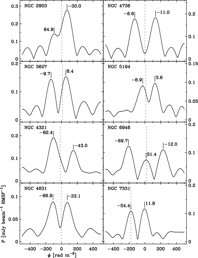 |
Figure 7: RM spectra extracted from the central regions of the indicated galaxies (coordinates are listed in Table 3). Features with tabulated characteristics are indicated with solid lines; the polarization angle at that value of RM is indicated. The Galactic foreground contribution (from Table 1) is indicated with dotted lines. |
In the case of NGC 4631, the split Faraday dispersion function may be
influenced by the almost edge-on aspect of the galaxy. The orientation
could lead to a large Faraday depth toward the nucleus, which might
also be responsible for the prominent areas of likely depolarization
throughout the disk plane. A connection of Faraday depth with the
outer disk orientation is not as obvious for the more face-on
targets. In fact, the largest observed splitting between the two
detected components is seen in NGC 6946, for which the disk
inclination is only 33![]() .
For a circum-nuclear dipole field, a
sign reversal would not occur in the vertical component, but
would only be expected to occur in the radial
component. This would be most apparent in an edge-on viewing
geometry. For a quadrupole field a sign reversal would be
expected to occur in both the radial and vertical directions,
and thus might be seen independent of the viewing angle. Although
neither edge-on nor face-on viewing geometries of the outer disk are
strongly preferred for witnessing this phenomenon, our sample size is
not large enough to draw general conclusions on a preferred
circum-nuclear field configuration. There is also no immediately
apparent trend with the type of nucleus. Nuclei with optical
(Ho et al. 1997) and MIR (Dale et al. 2006) emission
consistent with an AGN are just as likely to show split
profiles (4/11) when compared to nuclei which are classified as
non-AGN (3/10). Similar analysis, using
the RM-Synthesis technique, of a larger number of galaxies would
help to clarify the situation.
.
For a circum-nuclear dipole field, a
sign reversal would not occur in the vertical component, but
would only be expected to occur in the radial
component. This would be most apparent in an edge-on viewing
geometry. For a quadrupole field a sign reversal would be
expected to occur in both the radial and vertical directions,
and thus might be seen independent of the viewing angle. Although
neither edge-on nor face-on viewing geometries of the outer disk are
strongly preferred for witnessing this phenomenon, our sample size is
not large enough to draw general conclusions on a preferred
circum-nuclear field configuration. There is also no immediately
apparent trend with the type of nucleus. Nuclei with optical
(Ho et al. 1997) and MIR (Dale et al. 2006) emission
consistent with an AGN are just as likely to show split
profiles (4/11) when compared to nuclei which are classified as
non-AGN (3/10). Similar analysis, using
the RM-Synthesis technique, of a larger number of galaxies would
help to clarify the situation.
Based on our sample, a sufficient condition for the existence of a
multiply peaked nuclear Faraday disperion function is simply the
presence of a compact, polarized nuclear source. There are two
apparent exceptions to this pattern which deserve further
comment. NGC 7331 has split profiles but no compact nuclear
source. This particular galaxy exhibits split Faraday dispersion
functions throughout the inner disk, so the splitting noted here does not apply to a nucleus. Moreover, only one of the RM components in
NGC 7331 (the inner disk) is displaced significantly from the Galactic
foreground value, rather than both as seen toward polarized nuclear
sources. On the other hand, NGC 4569 has what appears to be a compact,
polarized nuclear source, but the nuclear Faraday dispersion function
is not obviously split. In this case there is some indication for
broadening of the profile toward the nucleus in the Faraday depth
coherence image described in Sect. 4.3;
it may be that there is splitting which is
only barely resolved with our RM resolution (
![]() ).
Further work to investigate nuclear polarization should be
performed at higher frequency, where the effects of internal
Faraday depolarization are less important, and Faraday thick regions
can be unambiguously distinguished from regions with multiple distinct Faraday depths. At higher frequencies, the width of the RMSF will
likely be broader than we have obtained here. Judicious combinations of observations at low and high frequency can lead to the recovery of
Faraday thick polarized flux. As pointed out by
Brentjens & de Bruyn (2005), the condition for recovering such flux is
).
Further work to investigate nuclear polarization should be
performed at higher frequency, where the effects of internal
Faraday depolarization are less important, and Faraday thick regions
can be unambiguously distinguished from regions with multiple distinct Faraday depths. At higher frequencies, the width of the RMSF will
likely be broader than we have obtained here. Judicious combinations of observations at low and high frequency can lead to the recovery of
Faraday thick polarized flux. As pointed out by
Brentjens & de Bruyn (2005), the condition for recovering such flux is
![]() .
.
5 Conclusions and outlook
We have presented linear polarization data measured in two broad frequency bands near 1400 and 1700 MHz in the WSRT-SINGS survey. The RM-Synthesis method was used to reconstruct the intrinsic properties of the polarized emission, obtaining and correcting for the Faraday depth contributions from both the Milky Way and the target galaxies themselves. The reconstructed Faraday dispersion functions were deconvolved using a technique similar to the CLEAN algorithm commonly utilized in synthesis imaging. The deconvolution was particularly important with the present observations, because the gap in frequency coverage between our two frequency bands causes the RM spread function (RMSF) to exhibit sidelobes at nearly the 80% level.
The results of these processing steps were used to derive maps of the linearly polarized flux in each of the target galaxies, and, in cases where sufficient flux was measured, to analyze the spatial distributions of Faraday rotation measures, which probe the component of the magnetic field along the line of sight, and polarization vectors, which probe the component of the magnetic field perpendicular to the line of sight. The Faraday rotation corrected polarization angles were used to generate maps of the magnetic fields perpendicular to the line of sight.
Linearly polarized emission was detected in 21 of the 28 galaxies considered in this investigation. The detected galaxies all have Hubble type between Sab and Sd; only three galaxies (out of 24) in this range of classification were undetected in polarized flux. All of the (albeit few) sample galaxies with Hubble type later than Sd or earlier than Sa were all undetected. We have not detected any circularly polarized emission from any of the galaxies.
The most prominent trend which has emerged through this analysis is that in all galaxies with spatially extended polarized emission, the azimuthally-binned polarized flux is consistently lowest along the receding major axis. For such a trend to appear in such a large and diverse sample of spiral galaxies implies that a common magnetic field geometry has been revealed. In Paper III, we attempt to model the observed azimuthal variations in both rotation measure and polarized flux, using toy models of axi- and bi-symmetric magnetic field configurations, with the additional possibility of a non-zero vertical component to the field. We find that such a magnetic field geometry can explain the azimuthal variation in polarized flux, its dependence on inclination, as well as the azimuthal variation in the rotation measures attributed to the target galaxies.
Another interesting feature was discovered in the galaxies with
prominent nuclear emission in both total power and linearly polarized
flux. The Faraday dispersion functions in those galaxies' cores show
indications of significant broadening and/or splitting, indicating the
presence either of spatially collocated synchrotron-emitting and
Faraday-rotating plasma, or distinct Faraday thin emitting regions
within the resolution element. At the wavelengths observed in this
survey, we are rather insensitive to significantly broadened Faraday
dispersion functions - these would appear (at best) as double-peaked
profiles. It is possible that all of these galaxies host Faraday
thick regions in their cores, but we are unable to make this
distinction. Observations at higher radio frequencies, where
depolarization issues are less significant, would clarify the
situation. What is clear, from the occurence of both positive and
negative net RMs (after accounting for the Galactic foreground
contribution), is that the polarized emission arises on either side of
a reversal of the LOS field, presumably reflecting a radially directed
field (either inward or outward) centered on the nucleus. Whether
the LOS magnetic field simply changes sign near the nucleus, or
polarized flux is present at an extended range of Faraday depth
(centered near
![]() ), is not clear with the present
observations.
), is not clear with the present
observations.
The techniques used here can be extended to observations performed at
other radio telescopes. In particular, the new class of telescopes
which are being built now and into the era of the SKA, will all
provide polarization data at excellent frequency resolution covering
wide bandwidth. These telescopes will provide data which is
excellently suited for use with the RM-Synthesis method, and will
enable the study of a larger sample of galaxies at greater
sensitivity, and improved resolution in the Faraday domain. Of
particular interest is the LOw Frequency ARray
(LOFAR; Falcke et al. 2007) array which is presently being
built, and will operate at frequency ranges between 30-80 and
120-240 MHz. At these low frequencies, we will have RM resolutions
of order
![]() and better (cf. the WSRT-SINGS RM resolution
and better (cf. the WSRT-SINGS RM resolution
![]() ), yielding sensitivity to far weaker magnetic field
structures in nearby galaxies (Beck 2008).
), yielding sensitivity to far weaker magnetic field
structures in nearby galaxies (Beck 2008).
Acknowledgements
We thank Michiel Brentjens for providing his RM-Synthesis software, and for several enlightening discussions. The Westerbork Synthesis Radio Telescope is operated by ASTRON (The Netherlands Institute for Radio Astronomy) with support from the Netherlands Foundation for Scientific Research (NWO). The Digitized Sky Surveys were produced at the Space Telescope Science Institute under U.S. Government grant NAG W-2166. The images of these surveys are based on photographic data obtained using the Oschin Schmidt Telescope on Palomar Mountain and the UK Schmidt Telescope. The plates were processed into the present compressed digital form with the permission of these institutions. We thank the anonymous referee for carefully reading the manuscript, and providing helpful comments which have improved the paper.
Appendix A: Deconvolution of the Faraday dispersion function
The Faraday dispersion function recovered using RM-Synthesis has
undesirable features resulting from the incomplete sampling in the
![]() domain. These effects can be reduced using a deconvolution procedure, similar to what is done in the synthesis imaging case. Here, we outline and justify our procedure in greater detail than was provided in Sect. 2.3.
domain. These effects can be reduced using a deconvolution procedure, similar to what is done in the synthesis imaging case. Here, we outline and justify our procedure in greater detail than was provided in Sect. 2.3.
There are two salient features of the RMSF: the width of the main lobe (
![]() ), and the sidelobe structure. In the WSRT-SINGS survey, the sampling function (see Fig. 1, panel e) can be described as two windows. The form of our RMSF can be likened to the interference pattern in a double-slit experiment. If the windows (slits) were infinitely narrow, the sidelobes would
have unit amplitude and the spacing would be inversely related to the distance in
), and the sidelobe structure. In the WSRT-SINGS survey, the sampling function (see Fig. 1, panel e) can be described as two windows. The form of our RMSF can be likened to the interference pattern in a double-slit experiment. If the windows (slits) were infinitely narrow, the sidelobes would
have unit amplitude and the spacing would be inversely related to the distance in ![]() between the windows. In fact, the locations on the
between the windows. In fact, the locations on the ![]() -axis of the sidelobes would be identical to the
-axis of the sidelobes would be identical to the ![]() ambiguity which would result from a standard rotation measure determination using the two
ambiguity which would result from a standard rotation measure determination using the two ![]() frequency samples alone. In actuality, the windows are made up of many individual frequency measurements, and therefore each effectively have a finite width. This provides a taper to damp down the sidelobes. But the windows are still relatively narrow compared to the distance between them, so the sidelobes remain rather high. It is therefore desirable to remove these sidelobes from
the recovered Faraday dispersion function, particularly in cases which may potentially contain multiple distinct sources or broadening along the
frequency samples alone. In actuality, the windows are made up of many individual frequency measurements, and therefore each effectively have a finite width. This provides a taper to damp down the sidelobes. But the windows are still relatively narrow compared to the distance between them, so the sidelobes remain rather high. It is therefore desirable to remove these sidelobes from
the recovered Faraday dispersion function, particularly in cases which may potentially contain multiple distinct sources or broadening along the ![]() axis. Before deconvolution, the sidelobe structure of a brighter component contaminates the response to fainter components, and may shift the location of peaks relative to their true position.
axis. Before deconvolution, the sidelobe structure of a brighter component contaminates the response to fainter components, and may shift the location of peaks relative to their true position.
The mechanism for performing this deconvolution is quite similar to
the CLEAN algorithm which is already well known from the
synthesis imaging case. We first describe the algorithm. Then we move
on to justifying our choice of working in a domain in which
![]() (see Eq. (5)).
Here we demonstrate that deconvolution in that
space is equivalent to deconvolution in the ``true'' measurement
space. Next we describe how a restoring RMSF was selected, and
conclude with some general remarks about the routine.
(see Eq. (5)).
Here we demonstrate that deconvolution in that
space is equivalent to deconvolution in the ``true'' measurement
space. Next we describe how a restoring RMSF was selected, and
conclude with some general remarks about the routine.
A.1 The deconvolution procedure
The algorithm, also described by Brentjens (2007), consists of the following steps:
- 1.
- in each spatial pixel, the complex (
 ,
, )
spectrum is cross-correlated with the complex RMSF. The location of the peak absolute value of the cross-correlation,
)
spectrum is cross-correlated with the complex RMSF. The location of the peak absolute value of the cross-correlation,  ,
is
noted;
,
is
noted;
- 2.
- if
 is greater than a user-defined cutoff, a shifted
and scaled version of the complex RMSF is subtracted from the
complex (,)
spectrum. The scaled RMSF is
is greater than a user-defined cutoff, a shifted
and scaled version of the complex RMSF is subtracted from the
complex (,)
spectrum. The scaled RMSF is
 ,
where g is a (real) gain factor.
,
where g is a (real) gain factor.
- 3.
- the value
 is stored as a ``clean component'';
- 4.
- steps 1-3 are repeated until the value of
is no
longer higher than the cutoff, or a maximum number of iterations
have been performed;
- 5.
- finally, the clean components are convolved with a restoring
Gaussian beam with a FWHM equal to
 (see A.3), and added to the residual
  .
The result is the deconvolved
spectrum.
.
The result is the deconvolved
spectrum.
A.2 Deconvolution in the ``shifted'' domain
We begin with the definitions of the dirty Faraday dispersion function in its unshifted (pure) form:
 |
(A.1) |
and its shifted form:
 |
(A.2) |
 |
(A.3) |
Noting that the factor
 |
(A.4) |
which is seen to be equivalent to:
 |
(A.5) |
In exactly the same way, it can be shown that the same relation holds for the RMSF:
 |
(A.6) |
We also must define
 |
(A.7) |
which is just the actual Faraday dispersion function multiplied by the ``shift'' factor.
Again beginning with the shifted, dirty Faraday dispersion function,
![\begin{displaymath}\tilde{F}'(\phi) = {\rm e}^{2i\phi\lambda_0^2}~\tilde{F}(\phi...
...}^{2i\phi\lambda_0^2}~\times~\left[F(\phi)~\ast~R(\phi)\right]
\end{displaymath}](/articles/aa/full_html/2009/32/aa12240-09/img327.png) |
(A.8) |
and incorporating the definition of a convolution,
 |
(A.9) |
We can now move the exponential inside the integral, and introduce two exponentials whose product is unity:
 |
(A.10) |
Rearranging,
 |
(A.11) |
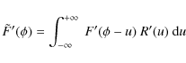 |
(A.12) |
which is just
| (A.13) |
This means that the shifted, dirty Faraday dispersion function is the convolution of the shifted RMSF
A.3 Selection of a restoring beam
The width of the main lobe of the RMSF,
![]() ,
reflects the
fact that we have only limited precision in our determination of the
Faraday depth of a polarized source. This is fundamentally related to
the sampling function. Thus, once we have extracted point source
components during the deconvolution routine, they must be replaced at
a resolution appropriate to the measured frequency domain. In other
words the point source model is convolved with a ``restoring
beam''. How does one choose the form of this restoring function?
,
reflects the
fact that we have only limited precision in our determination of the
Faraday depth of a polarized source. This is fundamentally related to
the sampling function. Thus, once we have extracted point source
components during the deconvolution routine, they must be replaced at
a resolution appropriate to the measured frequency domain. In other
words the point source model is convolved with a ``restoring
beam''. How does one choose the form of this restoring function?
By derotating to
![]() ,
Brentjens & de Bruyn (2005) show that the variation in the
imaginary part of the RMSF is minimized. In a sense, we have selected
a frame which rotates as a function of
,
Brentjens & de Bruyn (2005) show that the variation in the
imaginary part of the RMSF is minimized. In a sense, we have selected
a frame which rotates as a function of ![]() in (Q,U) space
such that the polarization vector stays along the Q axis as much as possible. We would like to choose a restoring function which is
equivalent to zeroing out the residual U response in this rotating
frame: in other words, asserting that we have in fact determined the
true rotation measure of the polarized source. (Recall, this is
equivalent to eliminating the sidelobes of the RMSF). Thus, we set the imaginary part of the restoring function to zero, and the real part to a Gaussian similar to the central lobe of the real part of the RMSF, in the rotating frame
in (Q,U) space
such that the polarization vector stays along the Q axis as much as possible. We would like to choose a restoring function which is
equivalent to zeroing out the residual U response in this rotating
frame: in other words, asserting that we have in fact determined the
true rotation measure of the polarized source. (Recall, this is
equivalent to eliminating the sidelobes of the RMSF). Thus, we set the imaginary part of the restoring function to zero, and the real part to a Gaussian similar to the central lobe of the real part of the RMSF, in the rotating frame
![]() .
Formally, we choose
.
Formally, we choose

a real-valued function, where
A.4 Practical considerations
Formally, this technique is straightforward. In the presence of noise, however, one must take care to properly treat the residuals and the CLEAN components which are returned by the deconvolution algorithm. In practice, the residuals are multiplied by the inverse shift factor (described above) separately. Then, the model is convolved with the restoring beam selected above, multiplied by the inverse shift factor, and added to the residuals. The final result is our deconvolved Faraday dispersion function, as used in this paper.
A final consideration is that the cubes should be reordered prior to
performing the deconvolution routine. This is because the routine
works not on individual image slices, but rather on spectra along the ![]() axis. Therefore it is considerably more efficient for the
routine to be able to read out spectra sequentially, instead of having to read through the full cube to construct each spectrum.
axis. Therefore it is considerably more efficient for the
routine to be able to read out spectra sequentially, instead of having to read through the full cube to construct each spectrum.
This RM-CLEAN algorithm has been implemented by us as a MIRIAD task and has been made publically available![]() . The task
typically takes less than 20 mn to operate on a pair of
(
. The task
typically takes less than 20 mn to operate on a pair of
(![]() ,
,![]() )
cubes with dimensions (
)
cubes with dimensions (
![]() )
on a dual 1.8 GHz Opteron system,
to the cutoff level described in Sect. 2.3.
)
on a dual 1.8 GHz Opteron system,
to the cutoff level described in Sect. 2.3.
References
- Beck, R. 2007, A&A, 470, 539 [NASA ADS] [CrossRef] [EDP Sciences] (In the text)
- Beck, R. 2008, Rev. Mex. Astron. Astrof. [arXiv:0804.4594] (In the text)
- Berkhuijsen, E. M., Horellou, C., Krause, M., et al. 1997, A&A, 318, 700 [NASA ADS] (In the text)
- Boulares, A., & Cox, D. P. 1990, ApJ, 365, 544 [NASA ADS] [CrossRef] (In the text)
- Braun, R. 1995, A&AS, 114, 409 [NASA ADS]
- Braun, R., Oosterloo, T. A., Morganti, R., Klein, U., & Beck, R. 2007, A&A, 461, 455 [NASA ADS] [CrossRef] [EDP Sciences] (In the text)
- Braun, R., Thilker, D., Walterbos, R., & Corbelli, E. 2009, ArXiv e-prints (In the text)
- Brentjens, M. A. 2007, Ph.D. Thesis, Rijksuniversiteit Groningen, Netherlands (In the text)
- Brentjens, M. A., & de Bruyn, A. G. 2005, A&A, 441, 1217 [NASA ADS] [CrossRef] [EDP Sciences] (In the text)
- Broten, N. W., MacLeod, J. M., & Vallee, J. P. 1988, Ap&SS, 141, 303 [NASA ADS] [CrossRef]
- Bureau, M., & Carignan, C. 2002, AJ, 123, 1316 [NASA ADS] [CrossRef]
- Burn, B. J. 1966, MNRAS, 133, 67 [NASA ADS] (In the text)
- Chyzy, K. T. 2008, A&A, 482, 755 [NASA ADS] [CrossRef] [EDP Sciences] (In the text)
- Chyzy, K. T., Soida, M., Bomans, D. J., et al. 2006, A&A, 447, 465 [NASA ADS] [CrossRef] [EDP Sciences] (In the text)
- Chyzy, K. T., Ehle, M., & Beck, R. 2007, A&A, 474, 415 [NASA ADS] [CrossRef] [EDP Sciences] (In the text)
- Condon, J. J., Cotton, W. D., Greisen, E. W., et al. 1998, AJ, 115, 1693 [NASA ADS] [CrossRef] (In the text)
- Dale, D. A., Smith, J. D. T., Armus, L., et al. 2006, ApJ, 646, 161 [NASA ADS] [CrossRef] (In the text)
- de Blok, W. J. G., Walter, F., Brinks, E., et al. 2008, AJ, 136, 2648 [NASA ADS] [CrossRef]
- de Vaucouleurs, G., de Vaucouleurs, A., Corwin, Jr., H. G., et al. 1991, Third Reference Catalogue of Bright Galaxies, 1-3, XII, 2069, 7 Figs. (New York: Springer-Verlag Berlin Heidelberg)
- Dolag, K., Vogt, C., & Enßlin, T. A. 2005, MNRAS, 358, 726 [NASA ADS] [CrossRef]
- Ehle, M., & Beck, R. 1993, A&A, 273, 45 [NASA ADS] (In the text)
- Falcke, H. D., van Haarlem, M. P., de Bruyn, A. G., et al. 2007, Highlights of Astronomy, 14, 386 [NASA ADS] (In the text)
- Gaensler, B. M., Haverkorn, M., Staveley-Smith, L., et al. 2005, Science, 307, 1610 [NASA ADS] [CrossRef] (In the text)
- Gardner, F. F., & Whiteoak, J. B. 1963, Nature, 197, 1162 [NASA ADS] [CrossRef] (In the text)
- Garrington, S. T., Leahy, J. P., Conway, R. G., et al. 1988, Nature, 331, 147 [NASA ADS] [CrossRef]
- Golla, G., & Hummel, E. 1994, A&A, 284, 777 [NASA ADS] (In the text)
- Greisen, E. W. 2003, in Astrophysics and Space Science Library, Astrophys. Space Sci. Libr., ed. A. Heck, 285, 109 (In the text)
- Han, J. L., & Qiao, G. J. 1994, A&A, 288, 759 [NASA ADS]
- Ho, L. C., Filippenko, A. V., & Sargent, W. L. W. 1997, ApJS, 112, 315 [NASA ADS] [CrossRef] (In the text)
- Horellou, C., Beck, R., Berkhuijsen, E. M., Krause, M., & Klein, U. 1992, A&A, 265, 417 [NASA ADS] (In the text)
- Hummel, E., Beck, R., & Dahlem, M. 1991, A&A, 248, 23 [NASA ADS] (In the text)
- Jarrett, T. H., Chester, T., Cutri, R., Schneider, S. E., & Huchra, J. P. 2003, AJ, 125, 525 [NASA ADS] [CrossRef]
- Johnston, S., Taylor, R., Bailes, M., et al. 2008, Exp. Astron., 22, 151 [NASA ADS] [CrossRef] (In the text)
- Jones, T. W., & O'Dell, S. L. 1977, ApJ, 214, 522 [NASA ADS] [CrossRef] (In the text)
- Kamphuis, J., & Briggs, F. 1992, A&A, 253, 335 [NASA ADS]
- Kennicutt, Jr., R. C. 1981, AJ, 86, 1847 [NASA ADS] [CrossRef] (In the text)
- Kennicutt, Jr., R. C., Armus, L., Bendo, G., et al. 2003, PASP, 115, 928 [NASA ADS] [CrossRef] (In the text)
- Laing, R. A. 1988, Nature, 331, 149 [NASA ADS] [CrossRef]
- Laing, R. A., Canvin, J. R., Cotton, W. D., Bridle, A. H., & Parma, P. 2006, Astron. Nachr., 327, 533 [NASA ADS] [CrossRef]
- Longair, M. S. 1994, High energy astrophysics. Vol. 2: Stars, the galaxy and the interstellar medium (In the text)
- McKee, C. F., & Ostriker, E. C. 2007, ARA&A, 45, 565 [NASA ADS] [CrossRef] (In the text)
- Miley, G. 1980, ARA&A, 18, 165 [NASA ADS] [CrossRef] (In the text)
- Murphy, E. J., Helou, G., Braun, R., et al. 2006, ApJ, 651, L111 [NASA ADS] [CrossRef] (In the text)
- Paturel, G., Petit, C., Prugniel, P., et al. 2003, A&A, 412, 45 [NASA ADS] [CrossRef] [EDP Sciences]
- Popping, A., & Braun, R. 2008, A&A, 479, 903 [NASA ADS] [CrossRef] [EDP Sciences] (In the text)
- Rand, R. J. 1994, A&A, 285, 833 [NASA ADS] (In the text)
- Ruzmaikin, A. A., & Sokoloff, D. D. 1979, A&A, 78, 1 [NASA ADS] (In the text)
- Sault, R. J., Teuben, P. J., & Wright, M. C. H. 1995, in Astronomical Data Analysis Software and Systems IV, ed. R. A. Shaw, H. E. Payne, & J. J. E. Hayes, ASP Conf. Ser., 77, 433 (In the text)
- Schwarz, U. J. 1978, A&A, 65, 345 [NASA ADS] (In the text)
- Shetty, R., & Ostriker, E. C. 2006, ApJ, 647, 997 [NASA ADS] [CrossRef] (In the text)
- Soida, M., Urbanik, M., Beck, R., Wielebinski, R., & Balkowski, C. 2001, A&A, 378, 40 [NASA ADS] [CrossRef] [EDP Sciences] (In the text)
- Soida, M., Beck, R., Urbanik, M., & Braine, J. 2002, A&A, 394, 47 [NASA ADS] [CrossRef] [EDP Sciences] (In the text)
- Sokoloff, D. D., Bykov, A. A., Shukurov, A., et al. 1998, MNRAS, 299, 189 [NASA ADS] [CrossRef] (In the text)
- Tamburro, D., Rix, H.-W., Walter, F., et al. 2008, AJ, 136, 2872 [NASA ADS] [CrossRef]
- Tüllmann, R., Dettmar, R.-J., Soida, M., Urbanik, M., & Rossa, J. 2000, A&A, 364, L36 [NASA ADS] (In the text)
- Vogt, C., Dolag, K., & Enßlin, T. A. 2005, MNRAS, 358, 732 [NASA ADS] [CrossRef]
- Walter, F., Brinks, E., de Blok, W. J. G., et al. 2008, AJ, 136, 2563 [NASA ADS] [CrossRef] (In the text)
- Wardle, J. F. C., & Kronberg, P. P. 1974, ApJ, 194, 249 [NASA ADS] [CrossRef] (In the text)
Footnotes
- ... 83
![[*]](/icons/foot_motif.png)
- Morphologically-determined position angle
- ...
(RMSF)
- This function was originally referred to as the rotation measure transfer function (RMTF) by Brentjens & de Bruyn (2005), but has since been relabeled to more accurately reflect its mathematical relationship to the Faraday dispersion function.
- ... available
- The RM-CLEAN procedure is available for download from http://www.astron.nl/~heald/software
All Tables
Table 1: Summary of survey galaxies.
Table 2: Discrete source rotation measures.
Table 3: Characteristics of split RM profiles in galaxy cores.
All Figures
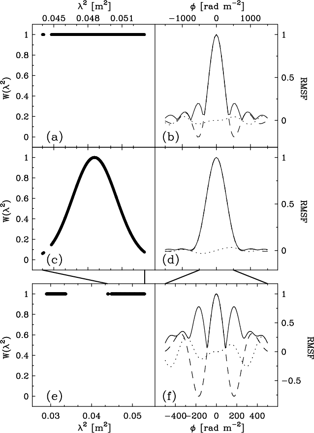 |
Figure 1:
RMSFs corresponding to the frequency coverage in the observations of NGC 628. RMSF values were calculated using the 22 cm band alone (untapered: a),b); tapered: c),d)) and in the combination of the 18 cm and 22 cm bands ( e),f)). In each row, the left panel shows the value of the weight function
|
| In the text | |
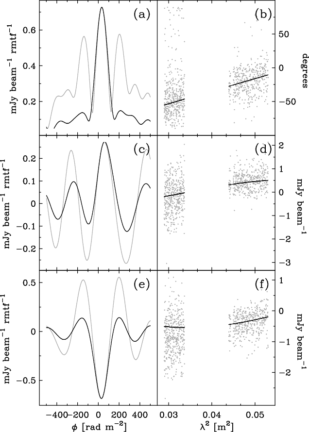 |
Figure 2:
Demonstration of the RM-CLEAN process for a relatively bright point source in the field of NGC 4125. Top: P, middle: Q, bottom: U. Gray lines are the dirty spectra; black lines are the cleaned spectra. A restoring RMSF with FWHM
|
| In the text | |
 |
Figure 3:
Demonstration of the RM-CLEAN process for a relatively bright point source in the field of NGC 7331. Top: P, middle: Q, bottom: U. Gray lines are the dirty spectra; black lines are the cleaned spectra. A restoring RMSF with FWHM
|
| In the text | |
![\begin{figure}
\par\includegraphics[width=15cm,clip]{12240f4a}
\end{figure}](/articles/aa/full_html/2009/32/aa12240-09/img148.png) |
Figure 4:
Images of sample galaxies. Contour levels (white) in Stokes I run from 0.1
|
| In the text | |
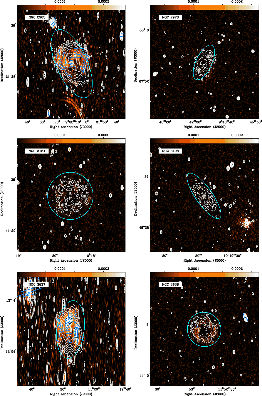 |
Figure 4: continued. |
| In the text | |
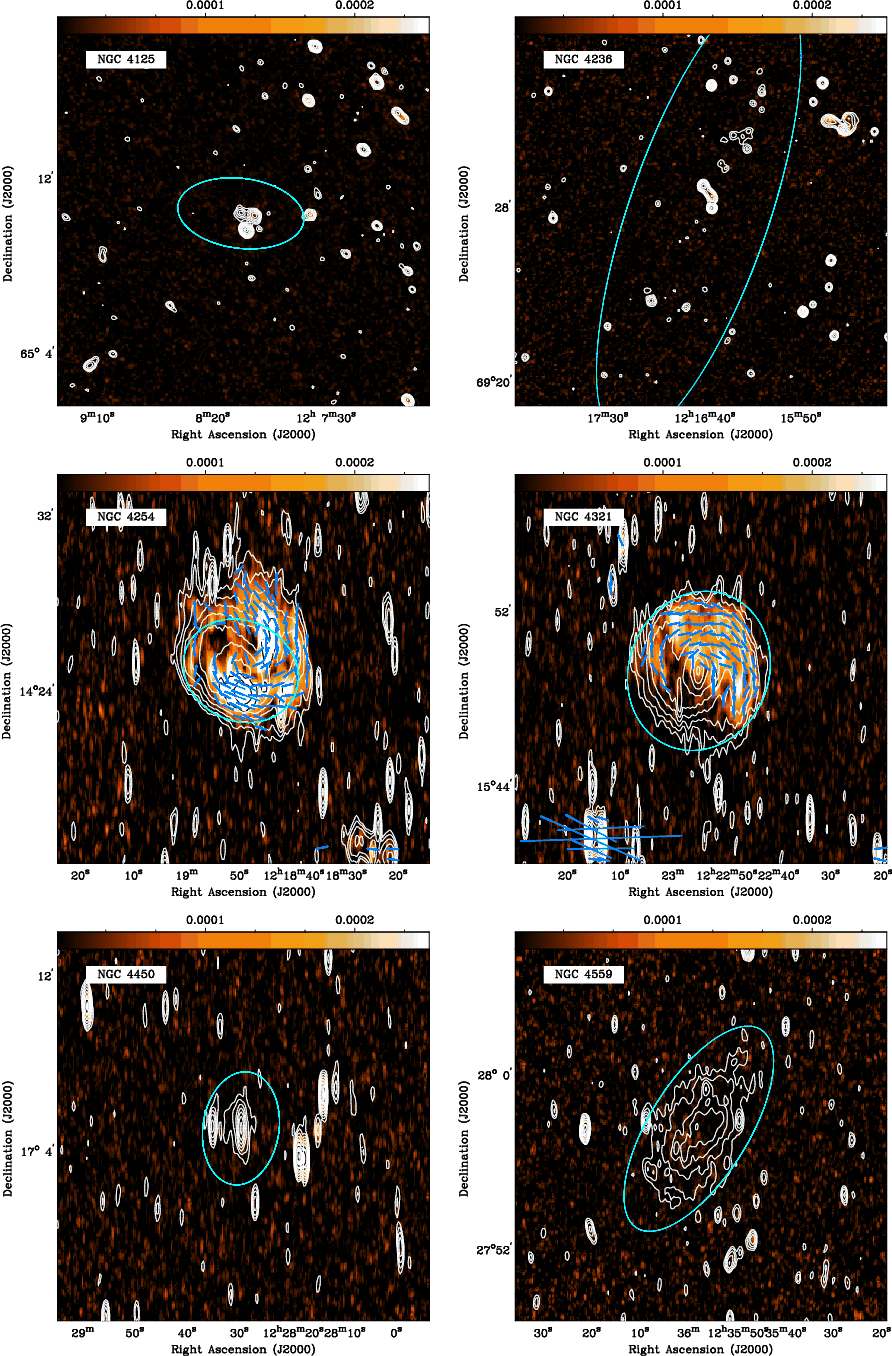 |
Figure 4: continued. |
| In the text | |
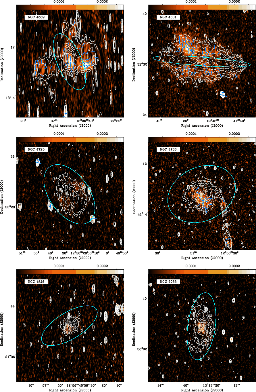 |
Figure 4: continued. |
| In the text | |
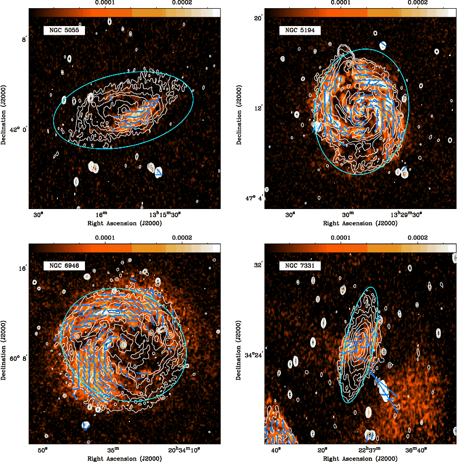 |
Figure 4: continued. |
| In the text | |
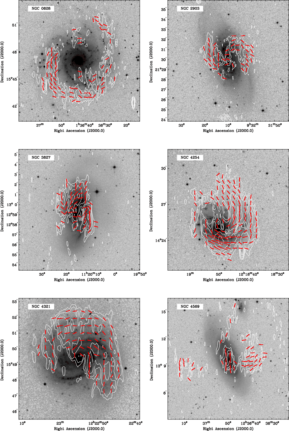 |
Figure 5:
Optical images of sample galaxies with extended polarized flux. The background images are red plates from the DSS-2, and are presented with a square-root color transfer to bring out the faint structures. Contour levels (white) of polarized intensity run from 50
|
| In the text | |
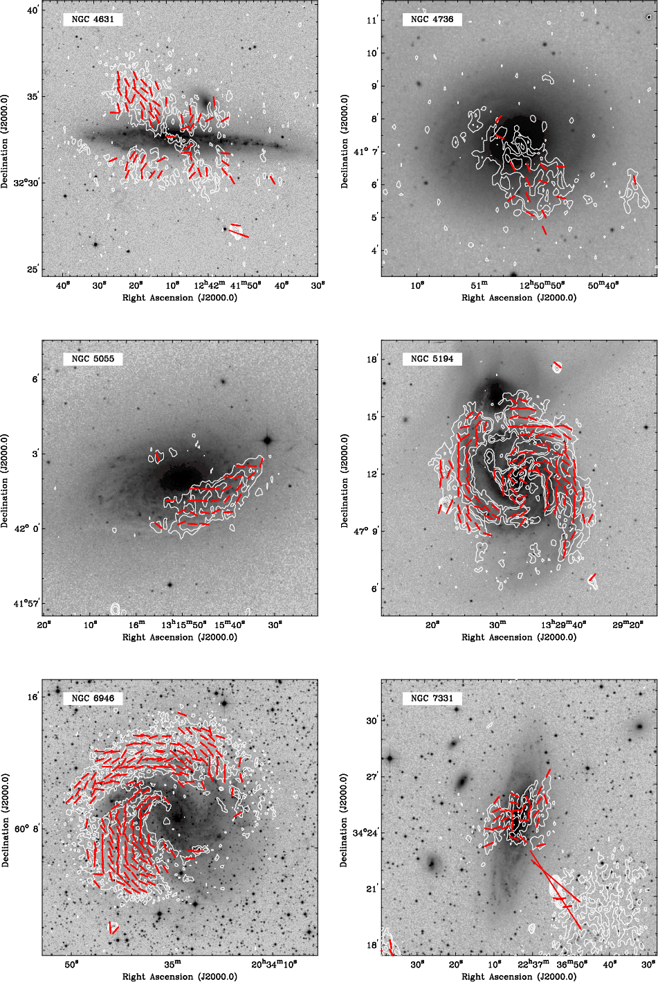 |
Figure 5: continued. |
| In the text | |
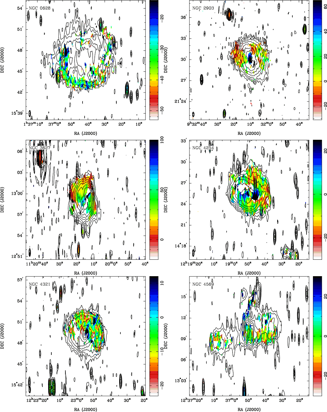 |
Figure 6:
Images of peak |
| In the text | |
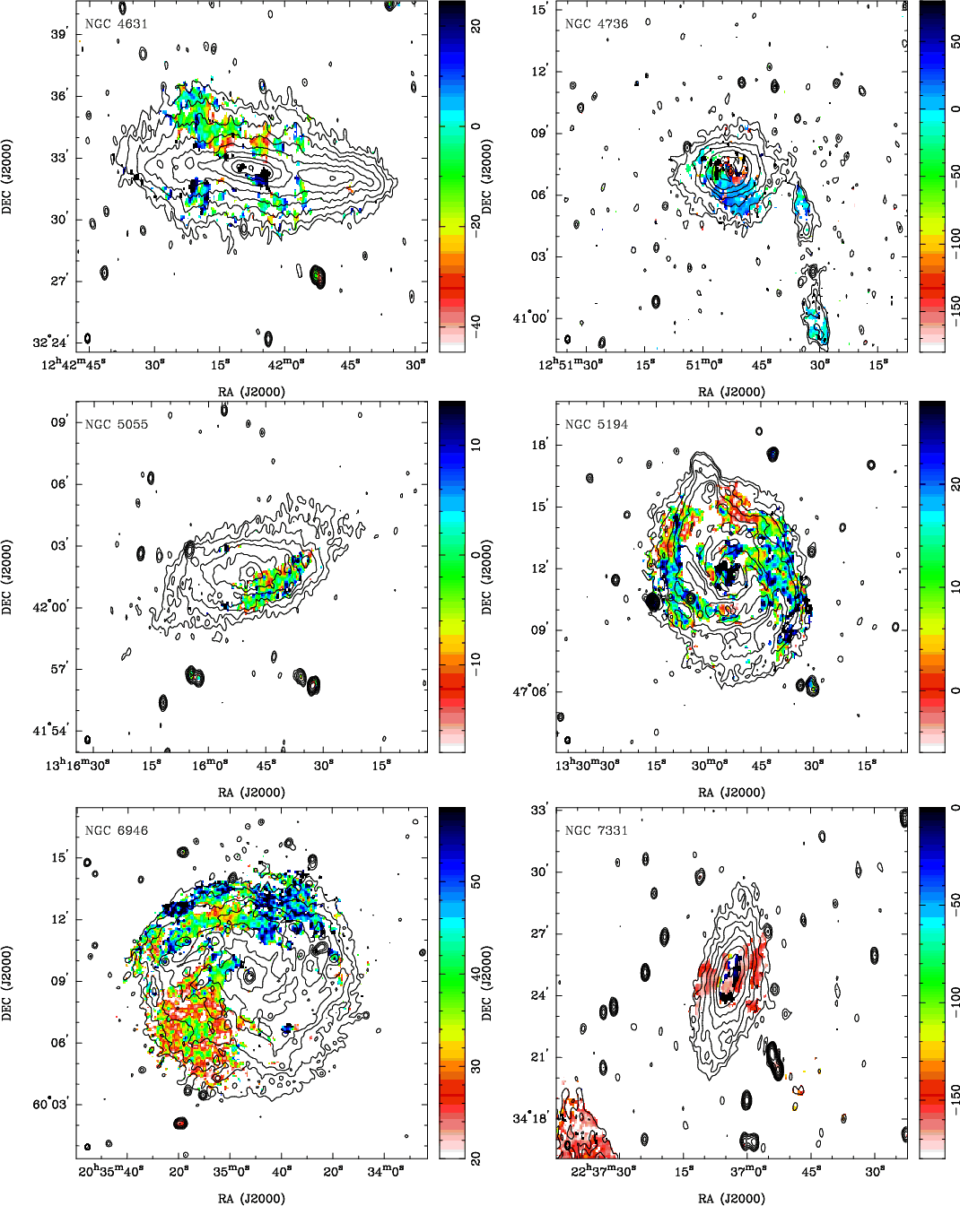 |
Figure 6: continued. |
| In the text | |
| |
Figure 7: RM spectra extracted from the central regions of the indicated galaxies (coordinates are listed in Table 3). Features with tabulated characteristics are indicated with solid lines; the polarization angle at that value of RM is indicated. The Galactic foreground contribution (from Table 1) is indicated with dotted lines. |
| In the text | |
Copyright ESO 2009
Current usage metrics show cumulative count of Article Views (full-text article views including HTML views, PDF and ePub downloads, according to the available data) and Abstracts Views on Vision4Press platform.
Data correspond to usage on the plateform after 2015. The current usage metrics is available 48-96 hours after online publication and is updated daily on week days.
Initial download of the metrics may take a while.