| Issue |
A&A
Volume 503, Number 2, August IV 2009
|
|
|---|---|---|
| Page(s) | 639 - 650 | |
| Section | Catalogs and data | |
| DOI | https://doi.org/10.1051/0004-6361/200810699 | |
| Published online | 15 June 2009 | |
A low-resolution near-infrared spectral library of M-, L-, and T-dwarfs![[*]](/icons/foot_motif.png)
L. Testi1,2
1 - INAF - Osservatorio Astrofisico di Arcetri, Largo E. Fermi 5, 50125 Firenze, Italy
2 -
European Southern Observatory, Karl Schwarzschild str. 2, 85748 Garching, Germany
Received 28 July 2008 / Accepted 6 April 2009
Abstract
We present complete near-infrared (0.85-2.45 ![]() m), low-resolution (
m), low-resolution (
![]() )
spectra of a sample of 54 disk M-, L-, and T-dwarfs with reliable optical or near infrared spectral-type classification from the literature. The observations were obtained with a prism-based optical element, the Amici device, which provides a complete spectrum of the source on the detector. Our observations indicate that low-resolution near-infrared spectroscopy can be used to determine the spectral classification of late-type field dwarfs in a fast but accurate way. We derive a set of near-infrared spectral indices
)
spectra of a sample of 54 disk M-, L-, and T-dwarfs with reliable optical or near infrared spectral-type classification from the literature. The observations were obtained with a prism-based optical element, the Amici device, which provides a complete spectrum of the source on the detector. Our observations indicate that low-resolution near-infrared spectroscopy can be used to determine the spectral classification of late-type field dwarfs in a fast but accurate way. We derive a set of near-infrared spectral indices
Key words: stars: low-mass, brown dwarfs - stars: fundamental parameters - infrared: stars
1 Introduction
We have witnessed an extraordinary evolution in the field of very low-mass stars and brown dwarfs. From being purely hypothetical objects, in only a few years, they have become first a curious oddity, following the first discoveries (Nakajima et al. 1995; Rebolo et al. 1995), then an entirely new class of stellar objects that required the definition of two new spectral classes: L (Martín et al. 1999; Kirkpatrick et al. 1999) and T (Kirkpatrick et al. 1999; Burgasser et al. 2002a; Geballe et al. 2002).
Very low-mass stars and brown dwarfs emit radiation mostly in the far red of the optical spectrum and in the near-infrared. For this reason the most successful strategies for identifying these objects have been based on near-infrared sky surveys, such as 2MASS (Kirkpatrick et al. 1999, 2000; Burgasser et al. 2002a) and DENIS (Delfosse et al. 1997; Tinney et al. 1998), and the red optical data of the SDSS (Fan et al. 2000). All of these surveys combined provide relatively good sensitivity in the appropriate bands and very wide area coverage. These two factors have allowed a sizeable number of nearby L- and T-type objects to be discovered, despite their intrinsic low luminosity.
Optical spectroscopic classification of the L-type objects, although feasible, has proven to be difficult because of the large amount of telescopes time required (Martín et al. 1999; Kirkpatrick et al. 1999). For this reason, several authors have attempted to relate the optical classification schemes to those in the near-infrared (e.g., Reid et al. 2001; Testi et al. 2001, hereafter T01; Geballe et al.2002). For T-dwarfs, optical classification is impractical and only near-infrared classification schemes have been proposed (e.g., Burgasser et al. 2002a, 2003; Geballe et al. 2002; Cushing et al. 2005). Because of the higher brightnesses of objects in the near infrared, these classification schemes, especially those based on low-resolution spectroscopy have proven to be very efficient.
The possibility of deriving a consistent method for near-infrared spectroscopic
classification of atmospheres with spectral types later than mid-M is also
attractive in confirming and classifying young, very low-mass objects in
star-forming regions. The combination of cool atmospheres and
environment extinction prevents the use of optical classification schemes
in many young star-forming regions. As an example, Natta et al. (2002)
and Testi et al. (2002) used low-resolution near-infrared spectroscopic classification methods to classify embedded young brown dwarfs in the ![]() -Ophiuchi star-forming
region.
-Ophiuchi star-forming
region.
In this paper, we present the results of very low-resolution near-infrared observations of 54 field dwarfs with spectral types in the range M3 to T8. The goal of these observations is to show that very low-resolution near-infrared spectroscopy allows one to classify these objects accurately and, by comparison with model atmospheres, to derive a good estimate of the atmospheric effective temperature. This work represents the extension and completion of our earlier work on field L-type dwarfs (T01). Bouvier et al. (2008) applied our spectral library to the classification young T-dwarfs in the Hyades cluster.
The paper is organized as follows. In Sect. 2, we describe the sample selection criteria, in Sect. 3, the observation setup and, in Sect. 4, our near-infrared cool dwarfs spectral library. In Sect. 5, we discuss a set of spectral indices useful to spectral classification. In Sect. 6, a comparison with model atmospheres is presented along with the method used to derive effective temperatures. In Sect. 7, we summarize the main conclusions of this study.
2 The sample
Field dwarfs were selected in order to obtain a coverage of the spectral types from M3V to T8V as uniformly as possible. The M-dwarfs were selected from the samples of Henry et al. (1994) and Kirkpatrick et al. (1995, 1999) according to observability, magnitude, and spectral-type classification. The selection of the L-dwarf sample was described in T01. The T-dwarfs were selected from the samples of Burgasser et al. (2000, 2002a), Leggett et al. (2000), and Strauss et al. (1999). The final sample consists of 54 cool field dwarfs, 17 M type, 26 L type, and 11 T type.
![\begin{figure}
\par\includegraphics[width=8.8cm,clip]{10699fg1.eps}
\end{figure}](/articles/aa/full_html/2009/32/aa10699-08/img14.png) |
Figure 1: Distribution of spectral types of the observed dwarfs. |
| Open with DEXTER | |
Table 1: Observed M-, L-, and T-dwarfs.
Adopted from the literature, the spectral classification of the M- and L-dwarfs is based on optical, red spectroscopy, while the T-dwarf spectral types are based on the near-infrared classification scheme of Burgasser et al. (2004). These authors provided a new classification scheme that refines, solves inconsistencies, and supersedes the previous schemes in Burgasser et al. (2002a) and Geballe et al. (2002). The distribution of spectral types in our sample is shown in Fig. 1. We emphasize that some authors have identified inconsistencies between the optical and infrared classification schemes of late dwarfs (e.g., Geballe et al. 2002); we did not explore these differences in our work but rather related our spectral library to the optical classification (where available). As we show in the following sections, this approach is quite successful and we do not find evidence that the use of our infrared spectral library could lead to ambiguous classification.
We decided not to include the coolest objects discovered most recently (Warren et al. 2007; Delorme et al. 2008) as the spectral classification of these remains uncertain. The possibility of extending the spectral library to the coolest objects will be considered when a larger number of them will be available and an appropriate spectral sequence will have been defined.
3 Observations and data reduction
The observational data were collected at the 3.58 m TNG
with the Near Infrared Camera and Spectrograph (NICS),
a cryogenic focal reducer designed as a near-infrared common-user instrument
for that telescope. The instrument is equipped with a Rockwell 10242HAWAII near-infrared array detector. Among the many imaging and spectroscopic
observing modes (Baffa et al. 2000, 2001), NICS offers a
high throughput, very low-resolution mode with an approximately constant
resolving power of ![]() 50, when the 1
50, when the 1
![]() wide slit is used. In this
mode, a prism-based optical element, the Amici device, is used to obtain a
complete 0.85-2.45
wide slit is used. In this
mode, a prism-based optical element, the Amici device, is used to obtain a
complete 0.85-2.45 ![]() m long-slit spectrum of the
astronomical source on
the detector (Baffa et al. 2001; Oliva 2003).
m long-slit spectrum of the
astronomical source on
the detector (Baffa et al. 2001; Oliva 2003).
The M- and T-dwarfs in our sample were observed
during several observing runs in the June 2001 to May 2003
period (see Table 1). We used the 0.5
![]() wide slit and the resulting
spectra have an effective resolution of
wide slit and the resulting
spectra have an effective resolution of ![]() 100 across the entire spectral range,
similarly the L-dwarfs observations reported in T01.
Integration times on source varied from a few to 25 min, depending on the
source brightness and sky transparency conditions. Wavelength calibration
was performed using an Argon lamp and deep telluric absorption features.
The telluric absorption was then removed by dividing each of the object
spectra by an A0 reference star spectrum observed at similar
airmass; the reference star was generally drawn from the Arnica standards
list (Hunt et al. 1998). Finally, flux normalization was completed using
a theoretical A0 star spectrum smoothed to the appropriate resolution.
No attempt was made to obtain an absolute flux calibration of the
final spectra. All the spectra discussed in this paper were normalized
to the average flux in the region 1.235-1.305
100 across the entire spectral range,
similarly the L-dwarfs observations reported in T01.
Integration times on source varied from a few to 25 min, depending on the
source brightness and sky transparency conditions. Wavelength calibration
was performed using an Argon lamp and deep telluric absorption features.
The telluric absorption was then removed by dividing each of the object
spectra by an A0 reference star spectrum observed at similar
airmass; the reference star was generally drawn from the Arnica standards
list (Hunt et al. 1998). Finally, flux normalization was completed using
a theoretical A0 star spectrum smoothed to the appropriate resolution.
No attempt was made to obtain an absolute flux calibration of the
final spectra. All the spectra discussed in this paper were normalized
to the average flux in the region 1.235-1.305 ![]() m. The shapes of the
final spectra were checked following the procedure outlined in T01.
For all 11 T-dwarfs in our sample and 2 of the L-dwarfs in T01,
low resolution, near-infrared spectra from IRTF/SpeX exist in the literature
(Burgasser et al. 2004; Burgasser 2006; Cruz et al. 2004
m. The shapes of the
final spectra were checked following the procedure outlined in T01.
For all 11 T-dwarfs in our sample and 2 of the L-dwarfs in T01,
low resolution, near-infrared spectra from IRTF/SpeX exist in the literature
(Burgasser et al. 2004; Burgasser 2006; Cruz et al. 2004![]() ).
A comparison shows that the spectra from the two libraries are
consistent within the uncertainties.
).
A comparison shows that the spectra from the two libraries are
consistent within the uncertainties.
4 The Amici spectral library
The primary goal of this work was to provide a library of
low-resolution near-infrared spectra of field dwarfs useful to
spectral classification![]() . In Figs. 2 and 3
we show the spectra of M- and T-dwarfs, respectively; the L-dwarf
spectra were shown already in T01 (their Fig. 1).
Absorption features related to metals (KI, NaI) and molecules
(TiO, FeH, CO) are visible in some of the spectra, depending on the
spectral type and signal-to-noise ratio of the data, but are usually not resolved.
The most prominent features in the spectra are those caused by
water vapour and, for the coolest spectral types, methane absorption.
These features, together with dust and H2 collision induced absorption,
determine the global shape of the spectra, which evolves distinctively from
early M to late T types. These features and their
theoretical interpretation have been discussed at length in the
literature (Allard et al. 2001; Reid et al. 2001;
Leggett et al. 2001; Burgasser et al. 2002a;
Geballe et al. 2002; Tsuji 2002) and are not rediscussed here.
. In Figs. 2 and 3
we show the spectra of M- and T-dwarfs, respectively; the L-dwarf
spectra were shown already in T01 (their Fig. 1).
Absorption features related to metals (KI, NaI) and molecules
(TiO, FeH, CO) are visible in some of the spectra, depending on the
spectral type and signal-to-noise ratio of the data, but are usually not resolved.
The most prominent features in the spectra are those caused by
water vapour and, for the coolest spectral types, methane absorption.
These features, together with dust and H2 collision induced absorption,
determine the global shape of the spectra, which evolves distinctively from
early M to late T types. These features and their
theoretical interpretation have been discussed at length in the
literature (Allard et al. 2001; Reid et al. 2001;
Leggett et al. 2001; Burgasser et al. 2002a;
Geballe et al. 2002; Tsuji 2002) and are not rediscussed here.
An important point for the study in this paper is that, even at this low spectral resolution, the spectra exhibit a smooth but distinctive variation as a function of spectral type. With the possible exception of a few spectra of the lower signal to noise ratio, the library of Amici field dwarf spectra can be used as a source of templates to derive spectral types for faint or embedded cool objects for which higher resolution infrared spectroscopy or optical spectroscopy is impractical. This method was applied with success in deriving spectral classifications of young embedded brown dwarfs (Natta et al. 2002; Testi et al. 2002; Bouvier et al. 2008).
![\begin{figure}
\par\includegraphics[width=17cm,clip]{10699fg2.eps}
\end{figure}](/articles/aa/full_html/2009/32/aa10699-08/img19.png) |
Figure 2:
NICS/Amici 0.85-2.45 |
| Open with DEXTER | |
![\begin{figure}
\par\includegraphics[width=17cm]{10699fg3.eps}
\end{figure}](/articles/aa/full_html/2009/32/aa10699-08/img20.png) |
Figure 3: Same as Fig. 2 (2MASS and SDSS names have been abbreviated). The spectral types are from Burgasser et al. (2002a). |
| Open with DEXTER | |
5 Spectral indices useful for classification
It is more practical to use a set of spectral indices when determining an approximate spectral classification. Many authors have proposed various near-infrared spectral indices that are useful in classifying of M-, L- and T-dwarfs (Reid et al. 2001; Burgasser et al. 2002a; Geballe et al. 2002). In T01, we discussed a set of indices based on our low-resolution near-infrared spectra that measure the slope of the residual continuum and the strength and shape of the main water vapour absorption bands. The numerical values of these indices for to our original sample of L-dwarfs, showed a tight correlation with the optically determined spectral types.
![\begin{figure}
\par\includegraphics[width=8.5cm,clip]{10699fg4.eps}
\end{figure}](/articles/aa/full_html/2009/32/aa10699-08/img21.png) |
Figure 4: Continuum-slope spectral indices, see T01 for the definition. Note that the indices indicate a progressive reddening of the continuum from the early M to the late L types, and a sharp blueing for T-dwarfs (see details in the text). |
| Open with DEXTER | |
![\begin{figure}
\par\includegraphics[width=7.8cm,clip]{10699fg5.eps}
\end{figure}](/articles/aa/full_html/2009/32/aa10699-08/img22.png) |
Figure 5:
Water bands spectral indices, see T01
for the definition. The indices sH2O |
| Open with DEXTER | |
In Figs. 4 and 5, we show the values of the
``continuum'' (sHJ and sKJ) and water-band indices (sH2O![]() ,
sH2O
,
sH2O![]() ,
sH2O
,
sH2O![]() ,
sH2O
,
sH2O![]() )
defined in T01
as a function of spectral type for our complete sample
of M-, L-, and T-dwarfs.
)
defined in T01
as a function of spectral type for our complete sample
of M-, L-, and T-dwarfs.
Both indices measuring the continuum slope (Fig. 4) show a tight correlation from the early M to the late L types corresponding to a progressive reddening of the spectrum. This trend is abruptly reversed for the T-dwarfs, which exhibit a strong blueing of the indices. This is caused by methane absorption and dust distribution in the atmosphere (see Allard et al. 2001). Methane absorption mainly affects the peak of the H and K bands, and our indices measure the depth of the methane absorption more than the continuum spectral slope of T-dwarfs. A similar trend is also evident for the broad-band colors (Kirkpatrick et al. 1999, 2000; Burgasser et al. 2002a),where the progressive reddening from early M to late L types is reversed for the T-dwarfs.
The water indices (Fig. 5) are very well correlated with spectral
type from the early M to the late L dwarfs. With the exception of the
sH2O![]() index, the other indices show a less tight correlation with
spectral type in the T-dwarf range, mainly because of the competing effect
of the methane absorption.
index, the other indices show a less tight correlation with
spectral type in the T-dwarf range, mainly because of the competing effect
of the methane absorption.
As discussed by Burgasser et al. (2002a) and Geballe et al. (2002), the classification of T-dwarfs is based on the spectral
features produced by the methane absorption. It is thus clear that the most
useful spectral classification indices are related to
the methane features. The success of the sH2O![]() index
in classifying T-dwarfs is due to its sensitivity to the
methane feature, which is very close to the water band at 1.15
index
in classifying T-dwarfs is due to its sensitivity to the
methane feature, which is very close to the water band at 1.15 ![]() m.
We do not define new methane indices for the spectral classification of
T-dwarfs, but instead show in Fig. 6 the value of the indices
defined by Burgasser et al. (2002a) computed using our spectra.
The values and correlation with spectral types are similar to the
results of Burgasser et al. and we emphasize here that these same indices
can be used to classify T-dwarfs using NICS/Amici spectra.
m.
We do not define new methane indices for the spectral classification of
T-dwarfs, but instead show in Fig. 6 the value of the indices
defined by Burgasser et al. (2002a) computed using our spectra.
The values and correlation with spectral types are similar to the
results of Burgasser et al. and we emphasize here that these same indices
can be used to classify T-dwarfs using NICS/Amici spectra.
![\begin{figure}
\par\includegraphics[width=9cm,clip]{10699fg6.eps}
\end{figure}](/articles/aa/full_html/2009/32/aa10699-08/img24.png) |
Figure 6:
Run of the H2O |
| Open with DEXTER | |
In Appendix A, we present an example of using two of the most reliable indices for the spectral classification of field dwarfs. Even if the method that we describe is reasonably accurate for many applications, we emphasize that spectral classification is most reliably achieved by comparing the complete spectra of the objects to be classified with the spectra of objects of known spectral type in the library.
5.1 Classification of reddened late-type objects
Low-resolution near-infrared spectroscopy is especially useful to the spectral classification of embedded cool objects, such as young brown dwarfs in star-forming regions (e.g., Testi et al. 2002; Natta et al. 2002). Other authors have discussed the issue of using dwarfs (or luminosity class V) as spectral standards for young pre-main-sequence objects (which have spectral properties of subgiants, or luminosity class IV). Wilking et al. (2003) showed that the spectral index they define for the classification of young M-type brown dwarfs has values closer to those of dwarfs rather than to giants (or luminosity class III). Other authors have highlighted the differences between young objects, field dwarfs, and giants (e.g., Kirkpatrick et al. 2006; Allers et al. 2007), A discussion of this problem is beyond the scope of this paper; we note, however, that, despite the difference in surface gravity, field M- and L-type dwarfs can be used, and indeed have been used, as comparison standards in classifying young embedded very low-mass stars and brown dwarfs (Natta et al. 2002; Testi et al. 2002). The computation of the spectral indices in the previous section for young objects in the SpeX Prism library are indeed consistent with their published spectral types (see Appendix A).
The use of spectral indices as defined in the previous section may be inpractical for reddened objects (see Appendix A). This is because, indices that measure the spectral slope at two wavelengths are systematically affected by extinction and any error in the dereddening of the spectra will be directly reflected in an error in the estimated spectral type.
To circumvent this uncertainty, Wilking et al. (1999) defined
a spectral index, called Q, which measures the strength of the water absorption
bands within the NIR K-band; it is formally insensitive to extinction and
exhibits a very good correlation with M subtypes. In this paper, we call
this index QK.
The use of this index with our Amici spectra is inpractical because it samples
regions of the spectrum close to 2.5 ![]() m that are usually affected
by very high background, detector non-linearity, and low signal-to-noise ratio
(in our Amici setup at the NICS/TNG). Additionally, the effectiveness of the
QK index is significantly reduced once the methane absorption become important
and suppresses the peak emission in the K-band.
m that are usually affected
by very high background, detector non-linearity, and low signal-to-noise ratio
(in our Amici setup at the NICS/TNG). Additionally, the effectiveness of the
QK index is significantly reduced once the methane absorption become important
and suppresses the peak emission in the K-band.
A similar index was defined by Lucas et al. (2001) for the H-band, which we call QH. This index shows a strong correlation between the M and mid-L types and for the late T-types where the methane absorption features in the H-band are more prominent. Its effectiveness is lower between the mid-L and mid-T range, where the correlation with spectral types is not so strong (see Fig. 7).
![\begin{figure}
\par\includegraphics[width=18.0cm]{10699fg7.eps}
\end{figure}](/articles/aa/full_html/2009/32/aa10699-08/img25.png) |
Figure 7:
Run of the IJ, IH, and IK indices as a function of
spectral type. Filled squares show the indices values for a
correct dereddening of the dwarf spectra; for each spectrum, the crosses
represent the value of the index assuming a dereddening with an
error of |
| Open with DEXTER | |
We explored the possibility of defining new indices at J, H, and K band
that are generally insensitive to errors in the determination of
extinction and subsequent dereddening of the observed spectra.
None of the indices that we define is as strictly reddening-independent as the
QH and QK indices defined by Lucas et al. (2001)
and Wilking et al. (1999), so all of them require
an estimate of the reddening and a dereddening of the spectrum before
the computation of the index and the estimate of the resulting spectral type.
The indices are defined as:
 |
(1) |
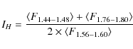 |
(2) |
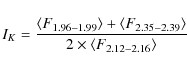 |
(3) |
where, as in T01,
6 Comparison with model atmospheres
Ultimately, the goal of the spectral classification of an observed object is to estimate its atmospheric physical parameters, mainly the effective temperature, surface gravity, and metallicity. Burgasser et al. (2004) showed metallicity differences in low-resolution infrared spectra of late dwarfs, although detailed empirical calibrations and extensive grids of model atmospheres of different metallities are still lacking, we therefore chose not to explore the effects of metallicity in this paper. The comparison of our low-resolution spectra with model libraries allows us to obtain meaningful estimates of effective temperature and surface gravity. To explore this possibility, we devised a procedure for fitting theoretical model spectra to our Amici spectra. The model grids used in this exercise are those of the Lyon group (Allard et al. 2001). The models span a wide range of effective temperatures and surface gravities for solar metallicities and a set of assumptions about both the dust location in the atmosphere and various types of molecular opacities. In our fits, we used three classes of models: the Dusty, Settl, and Cond models with AMES molecular opacities (see Allard et al. 2001; Leggett et al. 2001, 2002, for details on the models).
![\begin{figure}
\par\includegraphics[width=14.5cm,clip]{10699fg8.eps}
\end{figure}](/articles/aa/full_html/2009/32/aa10699-08/img32.png) |
Figure 8:
Effective temperature of the best-fit atmospheric
model as a function of spectral type. The triangles are obtained using
the ``q-estimator'' fitting method (Leggett et al. 2002), while
the crosses are the
results of a standard |
| Open with DEXTER | |
The atmosphere model fits to the observed spectra were performed following
a procedure similar to that of Leggett et al. (2002). For a given
observed spectrum, the model spectra were smoothed to the appropriate
resolution using a Gaussian function kernel
and resampled on the same wavelength grid as the observational data;
the model data were then scaled to the average flux of the observed spectrum
and two merit figures were computed: the ``q-estimator'' defined by Leggett
et al. (2002), and a classical ![]() .
For each observed spectrum, we
extracted the model spectra with the minimum value of ``q'' and
.
For each observed spectrum, we
extracted the model spectra with the minimum value of ``q'' and ![]() ;
in
general, with a few exceptions, the two best-fit models are either the
same or have very similar physical parameters. To avoid problems with low
signal-to-noise ratios and/or poor telluric correction, only spectral regions
outside the worse telluric absorption windows were used for all the steps
described above. This procedure was followed for the three class of models
considered: Dusty, Settl, and Cond.
;
in
general, with a few exceptions, the two best-fit models are either the
same or have very similar physical parameters. To avoid problems with low
signal-to-noise ratios and/or poor telluric correction, only spectral regions
outside the worse telluric absorption windows were used for all the steps
described above. This procedure was followed for the three class of models
considered: Dusty, Settl, and Cond.
The results of the three classes of atmospheric model fits were inspected for each object. With some individual exceptions, the general trend was consistent with the expectations: the Dusty models offer more reliable fits than the other classes, for M-type and early L-type dwarfs; the Settl models appear to be the most appropriate for late L-type and early T-type dwarfs; while the late type T-dwarf spectra are best fit by Cond models. We defined the ranges of applicability of the three classes of models as follows: Dusty for M to L4 dwarfs, Settl for L5 through T2, and Cond for T3 through T8. These boundaries were chosen in an arbitrary way, the different classes of models usually providing equivalent fits to the transition types. Some examples of the fit results are shown in Appendix B along with a table of the best-fit model parameters derived from the two methods.
In Fig. 8, we show the variation in the effective temperature of the
best-fit models as a function of the spectral type of the observed dwarf.
We find a generally good correlation and conclude that our model fitting
procedure can be used to estimate the effective temperature of the
observed dwarfs with an uncertainty of ![]() 100-150 K. This, of course,
neglects any possible systematic model uncertainties.
100-150 K. This, of course,
neglects any possible systematic model uncertainties.
In Fig. 8, we also show the results of our studies for the
L-dwarf range only (Marley et al. 2002; Burgasser 2001) and
down to the T-dwarf regime (Nakajima et al. 2004). All of these authors
derived the effective temperatures based on objects with known parallaxes
and by applying appropriate bolometric corrections to the measured magnitudes, and
derived the effective temperatures from the bolometric luminosities and
expected radius. It is comforting to verify that by fitting model atmospheres to the
observed spectra, we derive values that are in reasonable agreement with these
estimates. There are some possible systematic differences around the early and,
more noticeably, late L types. The effective temperatures that we derive for the
late L objects appear to be systematically ![]() 200 K above the other estimates.
We note that the L to T transition region is critical to the models;
in this range, it is indeed expected that the formation and vertical location of dust
clouds in the atmosphere will drastically affect the emerging near-infrared spectrum
(see e.g., the discussion in Ackerman & Marley 2001;
Burgasser et al. 2002b; and in Tsuji
et al. 2004). It is clear that to obtain a satisfactory description of
the atmospheres for these spectral types, the models need to take into
account the complicated physics of cloud formation and stratification (see e.g.,
Tsuji et al. 2004).
200 K above the other estimates.
We note that the L to T transition region is critical to the models;
in this range, it is indeed expected that the formation and vertical location of dust
clouds in the atmosphere will drastically affect the emerging near-infrared spectrum
(see e.g., the discussion in Ackerman & Marley 2001;
Burgasser et al. 2002b; and in Tsuji
et al. 2004). It is clear that to obtain a satisfactory description of
the atmospheres for these spectral types, the models need to take into
account the complicated physics of cloud formation and stratification (see e.g.,
Tsuji et al. 2004).
The surface gravity is far less tightly constrained by these types of fits than
to the effective temperatures. Our best-fit model parameters are within the ranges
expected for old field dwarfs (mostly
![]() ,
in cgs units). Significant
differences in the fits are expected for much lower gravity objects, such as
young very low-mass stars in star-forming regions or late-type Giants.
,
in cgs units). Significant
differences in the fits are expected for much lower gravity objects, such as
young very low-mass stars in star-forming regions or late-type Giants.
Even if our results are very consistent with other studies, we note that
our derivation of the photospheric parameters are also affected by the
uncertainties in the model atmospheres that we have used. As an example, using
different atmosphere models, Cushing et al. (2008) derived photospheric
temperatures for two of the T-dwarfs in our sample that are significantly lower
(![]() 300 K) than our estimates (and also lower than the Golimowski et al. 2004, fit).
300 K) than our estimates (and also lower than the Golimowski et al. 2004, fit).
7 Conclusions
We have presented a library of very low resolution, complete near-infrared spectra of M-, L-, and T-dwarfs in the solar neighborhood. We have confirmed and extended our earlier suggestions that low-resolution near-infrared spectroscopy is a powerful method for confirming and classifying faint dwarfs.
We have proposed a set of spectral indices that can be used to perform an accurate classification of faint dwarfs based on low-resolution spectra. Some of these indices are defined in such a way as to mitigate the effects of an incorrect or incomplete correction of the observed spectra for the effects of interstellar extinction.
The results of theoretical model atmosphere fits to our observed spectra have shown that the comparison between models and observations at this spectral resolution allows us to derive a reasonably accurate estimate of the effective temperature of the photospere. The values of the surface gravity derived from these model fits are within the expectations for old field dwarfs. Quantitative comparison with lower gravity objects is required to assess whether very low resolution spectra allow this additional atmospheric parameter to be constrained.
Acknowledgements
I would like to acknowledge early contributions to this work from F. Ghinassi, J. Licandro, A. Magazzù, A. Natta, E. Oliva, F. D'Antona, C. Baffa, G. Comoretto, S. Gennari, and F. Lisi. I also thank F. Allard for allowing the use of the cool dwarf atmosphere model spectra. This research has benefitted from the SpeX Prism Spectral Libraries, maintained by Adam Burgasser at http://www.browndwarfs.org/spexprism. This work has been partly supported by the MIUR grant 2002028843_001. Support from ASI grants ARS-99-15 and 1/R/27/00 to the Osservatorio di Arcetri is also gratefully acknowledged. It is a pleasure to thank the Arcetri and TNG technical staff and the TNG operators for their assistance during NICS commissioning and observing runs.
Appendix A: Example of spectral classification using the spectral indices
![\begin{figure}
\par\includegraphics[width=8.5cm]{10699fg9.eps}
\end{figure}](/articles/aa/full_html/2009/32/aa10699-08/img34.png) |
Figure A.1:
Spectral types estimated using the spectral indices (see text) compared with the catalogued spectral index for the SpeX spectra of field dwarfs. The solid line marks the locus of identical types, the dotted and dashed lines show interval representing
differences of |
| Open with DEXTER | |
![\begin{figure}
\par\includegraphics[width=8.5cm]{10699fg10.eps}
\end{figure}](/articles/aa/full_html/2009/32/aa10699-08/img35.png) |
Figure A.2: As Fig. A.1 but for young braown dwarfs in star forming regions. Note the different range in spectral types, which in this case only cover the range M6-M9. |
| Open with DEXTER | |
![\begin{figure}
\par\includegraphics[width=8.65cm]{10699fg11t.eps}\vspace*{1.5mm}
\includegraphics[width=8.65cm]{10699fg11b.eps}
\end{figure}](/articles/aa/full_html/2009/32/aa10699-08/img36.png) |
Figure A.3:
Top panel: as Fig. A.1 with added the derived spectral types assuming a dereddening error of
|
| Open with DEXTER | |
In this Appendix, we describe a possible pplicationof the spectral indices we have investigated in this paper in classifying cool photospheres. We note that spectral classification is by definition a process of classifying photospheres using global spectral properties. The use of spectral indices can only provide an approximate estimate of the spectral class of a given object and whenever possible a classification based on a direct comparison of the full spectrum with template spectra (such as those provided in our spectral library) should be used.
As an illustration, we use the indices sH2O![]() and sHJ to estimate the
spectral types of the field dwarfs in the SpeX Prism
library
and sHJ to estimate the
spectral types of the field dwarfs in the SpeX Prism
library![]() .
The procedure that we used is the following. We first estimated the spectral type using
the water index: if the derived spectral type was in the M- or L-type range this
provided directly the estimated spectral type of the object; if the estimated type was
in the T-type range, we used the sHJ index to estimate the spectral type.
In both cases to perform the spectral type estimate, we used quadratic fits to the
datapoints in our Amici spectral library (i.e., the points shown in
Figs. 4 and 5).
.
The procedure that we used is the following. We first estimated the spectral type using
the water index: if the derived spectral type was in the M- or L-type range this
provided directly the estimated spectral type of the object; if the estimated type was
in the T-type range, we used the sHJ index to estimate the spectral type.
In both cases to perform the spectral type estimate, we used quadratic fits to the
datapoints in our Amici spectral library (i.e., the points shown in
Figs. 4 and 5).
In Fig. A.1, we show the results of this procedure for the SpeX spectra of field M-, L-, and T-dwarfs. The procedure is able to assign a spectral type that is accurate to within one subclass for the majority of objects. No systematic offset or error is evident, even though very few objects show a discrepancy of more than two subclasses.
We have also tested the procedure for the SpeX spectra of young objects (see Fig. A.2), which are all in the very narrow range M6-M9. The classification using the spectral index is remarkably accurate with all the objects classified being within one spectral subclass of their assigned spectral type.
As noted in Sect. 5 of the main text, the values of the spectral indices
are affected by extinction. To illustrate the effect
of an incorrect correction for the extinction on the estimated spectral types, we
performed the same
computation as above for the SpeX dwarfs spectra but assuming an error in dereddening
of
![]() mag (and assuming the Cardelli et al. 1989, extinction
law). The results, shown in Fig. A.3 top panel, show that
the error introduced into the estimate of the spectral type is very large, making
the use of the spectral indices essentially useless. In contrast, if the estimate
of the spectral type is made using a quadratic fit to the reddening independent
index IH (as derived from our Amici spectral library), the
effect of the erroneous correction for extinction is essentially negligible
(Fig. A.3 bottom panel).
mag (and assuming the Cardelli et al. 1989, extinction
law). The results, shown in Fig. A.3 top panel, show that
the error introduced into the estimate of the spectral type is very large, making
the use of the spectral indices essentially useless. In contrast, if the estimate
of the spectral type is made using a quadratic fit to the reddening independent
index IH (as derived from our Amici spectral library), the
effect of the erroneous correction for extinction is essentially negligible
(Fig. A.3 bottom panel).
Table A.1:
Model atmospheres fitting results. For each object we
provide the effective temperature and the surface
gravity of the best fitting model with the ![]() and the q methods (see text).
and the q methods (see text).
Appendix B: Results and examples of model fits
We present in tabular format the results of the model atmosphere
fits to the observed spectra. We also provide some examples of the details of
the model fits and the ![]() surfaces.
surfaces.
![\begin{figure}
\par\includegraphics[width=17.0cm]{10699fg12.eps}
\end{figure}](/articles/aa/full_html/2009/32/aa10699-08/img39.png) |
Figure B.1:
Examples of model atmosphere fits to our observed near-infrared spectra.
Left panel: the observed spectra are shown as solid line, the best-fit model
is shown as a dotted line. The names and spectral types of the dwarfs are marked
together with the best-fit model atmosphere parameters. Right panel: |
| Open with DEXTER | |
![\begin{figure}
\par\includegraphics[width=17.0cm]{10699fg13.eps}
\end{figure}](/articles/aa/full_html/2009/32/aa10699-08/img40.png) |
Figure B.2:
``Dusty'' and ``Settl'' models fitted to an L5 and an L6 dwarf.
Left panel: the observed spectrum is shown as a solid line, the ``Dusty''
models as dotted lines and the ``Settl'' models as dashed lines.
The name of the dwarfs and the model parameters are marked on each panel.
Right panel: |
| Open with DEXTER | |
In Table B.1, we report for each star the best-fit model effective
temperature and surface gravity for both the ![]() and the q methods. The
results are presented for the range of applicability of the various models.
We also provide (in parentheses) the results of each class of models for
objects one subclass beyond their range of applicability.
and the q methods. The
results are presented for the range of applicability of the various models.
We also provide (in parentheses) the results of each class of models for
objects one subclass beyond their range of applicability.
![\begin{figure}
\par\includegraphics[width=17.0cm]{10699fg14.eps}
\end{figure}](/articles/aa/full_html/2009/32/aa10699-08/img41.png) |
Figure B.3:
``Settl'' and ``Cond'' models fitted to a T2 and a T3 dwarf.
Left panel: the observed spectrum is shown as a solid line, the ``Settl''
models as dotted lines and the ``Cond'' models as dashed lines.
The name of the dwarfs and the model parameters are marked on each panel.
Right panel: |
| Open with DEXTER | |
In Fig. B.1, we show the results of fitting the Lyon model
atmospheres to the observations of dwarfs well within the range of applicability
of the various models: ``Dusty'' models for an M 8.5 dwarf, ``Settl'' models for a
T1 dwarf, and ``Cond'' models for a T8 dwarf. The fits derived with the ![]() method
are shown; as noted in Sect. 6, no major differences appear if the
``q''-method is used. In the same figure, we also show the
method
are shown; as noted in Sect. 6, no major differences appear if the
``q''-method is used. In the same figure, we also show the ![]() surfaces for a
grid of models spanning a suitable range of effective temperatures and surface
gravities. We note that the effective temperature is more tightly
constrained by these fits than the surface gravity. It is not the purpose here to
discuss how well the models fit the observations and which observed
features are more difficult to reproduce. A comprehensive discussion of
these issues is provided in the series of papers by Allard et al. (2001),
Leggett et al. (2001, 2002), and Cushing et al. (2008).
What is useful to note is that our
spectral library can also be a useful benchmark for identifying shortcomings in
the models. As an example, the models cannot adequately fit the peak near 1.05
surfaces for a
grid of models spanning a suitable range of effective temperatures and surface
gravities. We note that the effective temperature is more tightly
constrained by these fits than the surface gravity. It is not the purpose here to
discuss how well the models fit the observations and which observed
features are more difficult to reproduce. A comprehensive discussion of
these issues is provided in the series of papers by Allard et al. (2001),
Leggett et al. (2001, 2002), and Cushing et al. (2008).
What is useful to note is that our
spectral library can also be a useful benchmark for identifying shortcomings in
the models. As an example, the models cannot adequately fit the peak near 1.05 ![]() m
in the late T-dwarfs, while they provide an excellent fit throughout the
remainder of the near-infrared domain.
m
in the late T-dwarfs, while they provide an excellent fit throughout the
remainder of the near-infrared domain.
In Figs. B.2 and B.3, we show examples of fits to dwarfs close to the transition of applicability of different classes of models. In these ranges, the different classes of models offer similar fits, each class with different types of shortcomings or successes. The model parameters, especially the effective temperature, do not differ significantly, except in the case of the T2 dwarf, where the ``Cond'' models offer a very poor fit to the observed spectrum.
References
- Ackerman, A. S., & Marley, M. S. 2001, ApJ, 556, 872 [NASA ADS] [CrossRef] (In the text)
- Allard, F., Hauschildt, P. H., Alexander, D. R., Tamanai, A., & Schweitzer, A. 2001, ApJ, 556, 357 [NASA ADS] [CrossRef] (In the text)
- Allers, K. N., Jaffe, D. T., Luhman, K. L., et al. 2007, ApJ, 657, 511 [NASA ADS] [CrossRef] (In the text)
- Baffa, C., Gennari, S., Lisi, F., et al. 2000, in The Scientific Dedication of the Telescopio Nazionale Galileo, Conference held in Santa Cruz de La Palma on November 3-5, 2000 (In the text)
- Baffa, C., Comoretto, G., Gennari, S., et al. 2001, A&A, 378, 722 [NASA ADS] [CrossRef] [EDP Sciences] (In the text)
- Basri, G., Mohanty, S., Allard, F., et al. 2000, ApJ, 538, 363 [NASA ADS] [CrossRef]
- Bouvier, J., Kendall, T., Meeus, G., et al. 2008, A&A, 481, 661 [NASA ADS] [CrossRef] [EDP Sciences] (In the text)
- Burgasser, A. J. 2001, Ph.D. Thesis, California Institute of Technology (In the text)
- Burgasser, A. J. 2006, AJ, 134, 1330 [NASA ADS] [CrossRef] (In the text)
- Burgasser, A. J., Kirkpatrick, J. D., Cutri, R. M., et al. 2000, ApJ, 531, L57 [NASA ADS] [CrossRef] (In the text)
- Burgasser, A. J., Kirkpatrick, J. D., Brown, M. E., et al. 2002a, ApJ (In the text)
- Burgasser, A. J., Marley, M. S., Ackerman, A. S., et al. 2002b, ApJ, 571, L151 [NASA ADS] [CrossRef] (In the text)
- Burgasser, A. J., Kirkpatrick, J. D., Liebert, J., & Burrows, A. 2003, ApJ, 594, 510 [NASA ADS] [CrossRef] (In the text)
- Burgasser, A. J., McElwain, M. W., Kirkpatrick, J. D., et al. 2004, AJ, 127, 2856 [NASA ADS] [CrossRef] (In the text)
- Burgasser, A. J., Geballe, T. R., Leggett, S. K., Kirkpatrick, J. D., & Golimowski, D. A. 2007, ApJ, 637, 1067 [NASA ADS] [CrossRef]
- Cardelli, J. A., Clayton, G. C., & Mathis, J. S. 1989, ApJ, 345, 245 [NASA ADS] [CrossRef] (In the text)
- Cruz, K. L., Burgasser, A. J., Reid, I. N., & Liebert, J. 2004, ApJ, 604, L61 [NASA ADS] [CrossRef] (In the text)
- Cushing, M. C., Rayner, T. J., & Vacca, W. D. 2005, ApJ, 623, 1115 [NASA ADS] [CrossRef] (In the text)
- Cushing, M. C., Marley, M. S., Saumon, D., et al. 2008, ApJ, 678, 1372 [NASA ADS] [CrossRef] (In the text)
- Delfosse, X., Tinney, C. G., Forveille, T., et al. 1997, A&A, 327, L25 [NASA ADS] (In the text)
- Delorme, P., Delfosse, X., Albert, L., et al. 2008, A&A, 482, 961 [NASA ADS] [CrossRef] [EDP Sciences] (In the text)
- Fan, X., Knapp, G. R., Strauss, M. A., et al. 2000, AJ, 119, 928 [NASA ADS] [CrossRef] (In the text)
- Geballe, T. R., Knapp, G. R., Leggett, S. K., et al. 2002, ApJ, 564, 466 [NASA ADS] [CrossRef] (In the text)
- Golimowski, D. A., Knapp, G. R., Strauss, M. A., et al. 2004, AJ, 127, 3516 [NASA ADS] [CrossRef] (In the text)
- Hunt, L. K., Mannucci, F., Testi, L., et al. 1998, AJ, 115, 2594 [NASA ADS] [CrossRef] (In the text)
- Henry, T. J., Kirkpatrick, J. D., & Simons, D. A. 1994, AJ, 108, 1437 [NASA ADS] [CrossRef] (In the text)
- Kirkpatrick, J. D., Henry, T. J., & Simons, D. A. 1995, AJ, 109, 797 [NASA ADS] [CrossRef] (In the text)
- Kirkpatrick, J. D., Reid, I. N., Liebert, J., et al. 1999, ApJ, 519, 802 [NASA ADS] [CrossRef] (In the text)
- Kirkpatrick, J. D., Reid, I. N., Liebert, J., et al. 2000, AJ, 120, 447 [NASA ADS] [CrossRef] (In the text)
- Kirkpatrick, J. D., Barman, T. S., Burgasser, A. J., et al. 2006, ApJ, 639, 1120 [NASA ADS] [CrossRef] (In the text)
- Leggett, S. K., Geballe, T. R., Fax, X., et al. 2000, ApJ, 536, L35 [NASA ADS] [CrossRef] (In the text)
- Leggett, S. K., Allard, F., Geballe, T. R., Hauschildt, P. H., & Schweitzer, A. 2001, ApJ, 548, 908 [NASA ADS] [CrossRef] (In the text)
- Leggett, S. K., Hauschildt, P. H., Allard, F., Geballe, T. R., & Baron, E. 2002, MNRAS, 332, 78 [NASA ADS] [CrossRef] (In the text)
- Lucas, P. W., Roche, P. F., Allard, F., & Hauschildt, P. H. 2001, MNRAS, 326, 695 [NASA ADS] [CrossRef] (In the text)
- Marley, M. S., Seager, S., Saumon, D., et al. 2002, ApJ, 568, 335 [NASA ADS] [CrossRef] (In the text)
- Martín, E. L., Delfosse, X., Basri, G., et al. 1999, AJ, 118, 2466 [NASA ADS] [CrossRef] (In the text)
- Nakajima, T., Oppenheimer, B. R., Kulkarni, S. R., et al. 1995, Nature, 378, 463 [NASA ADS] [CrossRef] (In the text)
- Nakajima, T., Tsuji, T., & Yanagisawa, K. 2004, ApJ, 607, 499 [NASA ADS] [CrossRef] (In the text)
- Natta, A., Testi, L., Comerón, F., et al. 2002, A&A, 393, 597 [NASA ADS] [CrossRef] [EDP Sciences] (In the text)
- Oliva, E. 2003, Mem. Sc. Astr. It., 74, 118 [NASA ADS] (In the text)
- Rebolo, R., Zapatero-Osorio, M. R., & Martín, E. 1995, Nature, 377, 129 [NASA ADS] [CrossRef] (In the text)
- Reid, I. N., Burgasser, A. J., Cruz, K. L., Kirkpatrick, J. D., & Gizis, J. E. 2001, AJ, 121, 1710 [NASA ADS] [CrossRef] (In the text)
- Strauss, M. A., Fan, X., Gunn, J. E., et al. 1999, ApJ, 522, L61 [NASA ADS] [CrossRef] (In the text)
- Testi, L., D'Antona, F., Ghinassi, F., et al. 2001, ApJ, 552, L147 [NASA ADS] [CrossRef] (T01) (In the text)
- Testi, L., Natta, A., Oliva, E., et al. 2002, ApJ, 571, L155 [NASA ADS] [CrossRef] (In the text)
- Tinney, C. G., Delfosse, X., Forveille, T., & Allard, F. 1998, A&A, 338, 1066 [NASA ADS] (In the text)
- Tokunaga, A., & Kobayashi, N. 1999, AJ, 117, 1010 [NASA ADS] [CrossRef] (In the text)
- Tsuji, T. 2002, ApJ, 575, 264 [NASA ADS] [CrossRef] (In the text)
- Tsuji, T., Nakajima, T., & Yanagisawa, K. 2004, ApJ, 607, 511 [NASA ADS] [CrossRef] (In the text)
- Warren, S. J., Mortlock, D. J., Leggett, S. K., et al. 2007, MNRAS, 381, 1400 [NASA ADS] [CrossRef] (In the text)
- Wilking, B. A., Greene, T. P., & Meyer, M. R. 1999, AJ, 117, 469 [NASA ADS] [CrossRef] (In the text)
- Wilking, B. A., Mikhail, A., Carlson, G., Meyer, M. R., & Greene, T. P. 2003, in Brown Dwarfs, ed. E. L. Martín, IAU Symp., 211, 97 (In the text)
Footnotes
- ... T-dwarfs
- All the spectra presented in this paper are only available in electronic form at the CDS via anonymous ftp to cdsarc.u-strasbg.fr (130.79.128.5) or via http://cdsweb.u-strasbg.fr/cgi-bin/qcat?J/A+A/503/639
- ...2004
- Available at http://www.browndwarfs.org/spexprism
- ... classification
- The complete Amici spectral library, including the data published in T01, is available at CDS, see footnote to the frontpage of this paper.
- ...
library
- http://www.browndwarfs.org/spexprism
All Tables
Table 1: Observed M-, L-, and T-dwarfs.
Table A.1:
Model atmospheres fitting results. For each object we
provide the effective temperature and the surface
gravity of the best fitting model with the ![]() and the q methods (see text).
and the q methods (see text).
All Figures
| |
Figure 1: Distribution of spectral types of the observed dwarfs. |
| Open with DEXTER | |
| In the text | |
| |
Figure 2:
NICS/Amici 0.85-2.45 |
| Open with DEXTER | |
| In the text | |
| |
Figure 3: Same as Fig. 2 (2MASS and SDSS names have been abbreviated). The spectral types are from Burgasser et al. (2002a). |
| Open with DEXTER | |
| In the text | |
| |
Figure 4: Continuum-slope spectral indices, see T01 for the definition. Note that the indices indicate a progressive reddening of the continuum from the early M to the late L types, and a sharp blueing for T-dwarfs (see details in the text). |
| Open with DEXTER | |
| In the text | |
| |
Figure 5:
Water bands spectral indices, see T01
for the definition. The indices sH2O |
| Open with DEXTER | |
| In the text | |
| |
Figure 6:
Run of the H2O |
| Open with DEXTER | |
| In the text | |
| |
Figure 7:
Run of the IJ, IH, and IK indices as a function of
spectral type. Filled squares show the indices values for a
correct dereddening of the dwarf spectra; for each spectrum, the crosses
represent the value of the index assuming a dereddening with an
error of |
| Open with DEXTER | |
| In the text | |
| |
Figure 8:
Effective temperature of the best-fit atmospheric
model as a function of spectral type. The triangles are obtained using
the ``q-estimator'' fitting method (Leggett et al. 2002), while
the crosses are the
results of a standard |
| Open with DEXTER | |
| In the text | |
| |
Figure A.1:
Spectral types estimated using the spectral indices (see text) compared with the catalogued spectral index for the SpeX spectra of field dwarfs. The solid line marks the locus of identical types, the dotted and dashed lines show interval representing
differences of |
| Open with DEXTER | |
| In the text | |
| |
Figure A.2: As Fig. A.1 but for young braown dwarfs in star forming regions. Note the different range in spectral types, which in this case only cover the range M6-M9. |
| Open with DEXTER | |
| In the text | |
| |
Figure A.3:
Top panel: as Fig. A.1 with added the derived spectral types assuming a dereddening error of
|
| Open with DEXTER | |
| In the text | |
| |
Figure B.1:
Examples of model atmosphere fits to our observed near-infrared spectra.
Left panel: the observed spectra are shown as solid line, the best-fit model
is shown as a dotted line. The names and spectral types of the dwarfs are marked
together with the best-fit model atmosphere parameters. Right panel: |
| Open with DEXTER | |
| In the text | |
| |
Figure B.2:
``Dusty'' and ``Settl'' models fitted to an L5 and an L6 dwarf.
Left panel: the observed spectrum is shown as a solid line, the ``Dusty''
models as dotted lines and the ``Settl'' models as dashed lines.
The name of the dwarfs and the model parameters are marked on each panel.
Right panel: |
| Open with DEXTER | |
| In the text | |
| |
Figure B.3:
``Settl'' and ``Cond'' models fitted to a T2 and a T3 dwarf.
Left panel: the observed spectrum is shown as a solid line, the ``Settl''
models as dotted lines and the ``Cond'' models as dashed lines.
The name of the dwarfs and the model parameters are marked on each panel.
Right panel: |
| Open with DEXTER | |
| In the text | |
Copyright ESO 2009
Current usage metrics show cumulative count of Article Views (full-text article views including HTML views, PDF and ePub downloads, according to the available data) and Abstracts Views on Vision4Press platform.
Data correspond to usage on the plateform after 2015. The current usage metrics is available 48-96 hours after online publication and is updated daily on week days.
Initial download of the metrics may take a while.