Corrections of Sun-as-a-star p-mode frequencies for effects of the solar cycle

A.-M. Broomhall; W. J. Chaplin; Y. Elsworth; S. T. Fletcher; R. New

doi:10.1051/0004-6361/200912286

Home

All issues

Volume 503 / No 1 (August III 2009)

A&A, 503 1 (2009) 241-245

Full HTML

Free Access

Issue		A&A Volume 503, Number 1, August III 2009


Page(s)		241 - 245
Section		The Sun
DOI		https://doi.org/10.1051/0004-6361/200912286
Published online		23 June 2009

Corrections of Sun-as-a-star p-mode frequencies for effects of the solar cycle
(Research Note)

A.-M. Broomhall¹ - W. J. Chaplin¹ - Y. Elsworth¹ - S. T. Fletcher² - R. New²

1 - School of Physics and Astronomy, University of Birmingham, Edgbaston, Birmingham B15 2TT, UK
2 - Faculty of Arts, Computing, Engineering and Sciences, Sheffield Hallam University, Sheffield S1 1WB, UK

Received 6 April 2009 / Accepted 10 June 2009

Abstract
Solar p-mode frequencies vary with solar activity. It is important to take this into account when comparing the frequencies observed from epochs that span different regions of the solar cycle. We present details of how to correct observed p-mode frequencies for the effects of the solar cycle. We describe three types of correction. The first allows mode frequencies to be corrected to a nominal activity level, such as the canonical quiet-Sun level. The second accounts for the effect on the observed mode frequencies, powers, and damping rates of the continually varying solar cycle and is pertinent to frequencies obtained from very long data sets. The third corrects for Sun-as-a-star observations not seeing all components of the modes. Suitable combinations of the three correction procedures allow the frequencies obtained from different sets of data to be compared and enable activity-independent inversions of the solar interior. As an example of how to apply the corrections we describe those used to produce a set of definitive Sun-as-a-star frequencies.

Key words: methods: data analysis - Sun: activity - Sun: helioseismology - Sun: oscillations

1 Introduction

The Birmingham Solar Oscillations Network (BiSON) observes Sun-as-a-star Doppler velocities. BiSON data can, therefore, be used to determine the frequencies of low-degree (low-l) oscillations. Low-l oscillations are particularly important as they are the only p modes that penetrate the solar core.

Accurate and precise solar p-mode frequencies are often determined from time series that contain many years of data. One drawback to examining such long data sets is that, because of the 11-yr solar cycle, they must span a wide range of different activity levels. Since solar p-mode frequencies, lifetimes, powers, and peak asymmetries all vary systematically with solar activity (Howe 2008, and references therein) care must be taken when analysing the mode parameters obtained from long sets of data. For example, between solar maximum and minimum the frequency of a low-l mode at approximately $3000~\rm\mu Hz$ can change by as much as $1~\rm\mu Hz$ , an amount that is far greater than the errors associated with frequency estimates.

Broomhall et al. (2009) has recently published a list of definitive low-l frequencies that were obtained from $8640~\rm d$ of BiSON data. The authors list the raw frequencies, which were determined directly from the data by fitting profiles to the frequency-power spectrum. Broomhall et al. also quote frequencies that have been corrected for various solar cycle effects. This paper describes, in detail, how these corrections were made in a manner that will allow the reader to reproduce the corrections with their own data. This will allow comparisons between the frequencies obtained from data sets that were observed at different epochs and consequently different activity levels.

We begin, in Sect. 2, by describing the well-known linear solar cycle correction that can be used to correct mode frequencies to a nominal activity level. Then, in Sect. 3, we describe how to determine the ``devil-in-the-detail'' correction that accounts for cross-talk between the variations of different mode parameters with the solar cycle, and the distribution of activity levels over the period of observations. Finally, Sect. 4 describes a correction that is necessary when using Sun-as-a-star observations because not all mode components are detectable.

2 Linear solar cycle correction

The raw frequencies determined for two sets of data will be different if they were observed at different epochs. To allow frequencies from different periods of time to be compared, a solar cycle correction must be performed. This correction also allows the frequencies that would have been observed at the canonical quiet Sun level to be determined. The correction is based on the assumption that variations in global activity indices can be used as proxies for low-l frequency shifts. We also assume that the correction can be parameterised as a linear function of the chosen activity measure. For the 10.7-cm radio flux (Tapping & Detracey 1990), these assumptions are robust (Chaplin et al. 2004c) at the level of precision of the data. Chaplin et al. (2007) find that the NOAA Mg II H core-to-wing ratio (Viereck et al. 2001) is predominantly a better proxy for making solar cycle corrections. However, we found that the fill of the Mg II data was too sparse to use here.

Let $\nu_{n,l}$ be the set of fitted frequencies determined using data that were observed during a time when the mean activity level was $\langle A(t)\rangle$ . For example, the mean 10.7-cm radio flux observed in the 8640-d time series examined by Broomhall et al. (2009) was $\langle A(t)\rangle=118$ $\times$ $10^{-22}~\rm W~m^{-2}~Hz^{-1}$ . (For the remainder of this paper we refer to $10^{-22}~\rm W~m^{-2}~Hz^{-1}$ as radio flux units, RFU.) This value of $\langle A(t)\rangle$ has been calculated taking into account any gaps that were present in the BiSON time series (e.g. due to inclement weather and very occasionally instrumental problems). Let $\langle A(t) \rangle_{\rm c}$ be the activity level we wish to correct to. For example, Broomhall et al. quote frequencies that have been corrected to the canonical quiet-Sun value of the radio flux, which is fixed, from historical observations, at $\langle A(t)\rangle_{\rm c}=64~\rm RFU$ (Tapping & Detracey 1990). The linear solar cycle correction, $\delta\nu_{n,l}$ , is given by

$\begin{displaymath}% \delta\nu_{n,l}=-g_l\mathcal{F}(\nu)\left[\langle A(t)\rangle-\langle A(t)\rangle_{\rm c}\right], \end{displaymath}$

(1)

where g_l are l-dependent factors that calibrate the size of the shift and were determined in the manner described below. The $\mathcal{F}(\nu)$ in Eq. (1) is a function that allows for the dependence of the shift on mode frequency. We have used the same frequency dependence as was determined by Chaplin et al. (2004c,b). The calculated $\delta\nu_{n,l}$ can be added to the set of frequencies, $\nu_{n,l}$ , to obtain frequencies that are corrected to a mean activity level of $\langle A(t) \rangle_{\rm c}$ .

Table 1: Values of g_l used to make the linear solar cycle corrections in Broomhall et al. (2009).

To determine g_l the 8640-d set of BiSON data was split into 20 contiguous $432~\rm d$ segments. To uncover the dependence of the solar-cycle frequency shifts on the 10.7-cm radio flux mode frequencies were determined for each of these 20 time series in the manner described by Chaplin et al. (2004c). The gradient of the linear relationship between activity and frequency varies significantly with l because of the spatial dependence of the surface activity. Table 1 gives the values of g_l used in Broomhall et al. (2009). Figure 1 shows the linear frequency shifts, $\delta\nu_{n,l}$ , that were applied to the 8640-d BiSON data to correct the frequencies to a mean activity level of $64~\rm RFU$ .

The errors on $\delta\nu_{n,l}$ are dominated by the uncertainties associated with g_l. These errors need to be propagated through to the corrected frequencies and so the corrected uncertainties are of the order of 10 per cent larger than those associated with the raw fitted frequencies, $\nu_{n,l}$ .

$\begin{figure} \par\includegraphics[height=4cm, clip]{12286fg1} \end{figure}$	Figure 1: Linear corrections that were applied to the frequencies observed in the 8640-d time series, where the average activity level was $118~\rm RFU$ , to obtain frequencies correct for the canonical quiet-Sun level of $64~\rm RFU$ .
Open with DEXTER

It is possible that the true relationship between the observed frequency shifts and solar activity is quadratic or even of higher order. However, we do not find a higher-order relationship when we analyse the BiSON frequency shifts i.e., a linear relationship provides the best fit, given the precision in the BiSON frequency shifts. In order to ensure our correction procedure is internally consistent, we use BiSON shifts and a linear calibration.

An alternative approach is to use separate corrections for the rising and falling phases of the cycle. Chaplin et al. (2004c) show that there is a significant difference in the slope of the linear relationship between the rising and falling phases of the solar cycle. More recently, Jain et al. (2009) found, when studying modes of intermediate degree, that different slopes are required to accurately describe the observed changes in frequency when the cycle is split into different phases. Such an approach would be worthwhile if the data for which the solar cycle corrections are being made span only a rising or a falling phase.

However, the time series considered by Broomhall et al. (2009) spans 8640 d, including two rising phases and two falling phases. To test whether it was advantageous to fit the phases separately we have split the $432~\rm d$ time series into two sets, one for the rising phases and one for the falling phases. A linear fit between frequency shift and activity was performed for each set. A weighted mean of the linear corrections for the two phases was then calculated, where the weights corresponded to the proportion of the 8640 d spent in each phase. We found that for theoretical modes at $3000~\rm\mu Hz$ with l in the range 0-3 the two-phase frequency correction was in good agreement (within $1\sigma$ ) of the corrections found when a single linear fit was applied. Furthermore, the error bars associated with the two different correction approaches were similar in size. In other words, when considering a long time series that spans both rising and falling phases of the cycle it is more than adequate to use a single linear fit because the differences between the rising and falling phases are averaged.

3 Devil-in-the-detail and activity distribution correction

3.1 A description of the devil-in-the-detail effect

The linear solar cycle correction assumes that the observed mode frequencies correspond to an unweighted average of the time-varying frequencies. However, Chaplin et al. (2008) found that when analysing long data sets this is not the case. Long time series span, at the very least, a sizeable fraction of the 11-yr solar activity cycle. The data examined by Broomhall et al. (2009) is a good example of such a time series as it spans more than two complete solar cycles. Chaplin et al. (2008) find that the frequencies observed in long time series are biased by a cross-talk effect that has its origins in the simultaneous variations of mode frequencies, powers, and linewidths over the solar cycle. Chaplin et al. call this bias to the observed frequencies the ``devil-in-the-detail'' effect and we now describe in detail why this effect is observed.

Consider a simplistic scenario where only the mode frequencies change with time. The observed frequency of a mode is then determined by the activity levels observed over the total period of observations and the unshifted frequency of the mode in question. Now consider the fictitious scenario where we have 100 d of data and on 99 of the days the solar activity level is constant. Then on the $100{\rm th}$ day the activity level doubles.

The final observed profile of a mode is well represented by the sum of the mode profiles observed on each of the 100 d, normalised by the length of the observations. For the first 99 d of our fictitious time series the same profile is observed. However, on the last day the peak frequency of the mode profile will be shifted by an amount, given by Eq. (1), which is dependent on the mode's degree and frequency. The influence of the final day on the peak frequency of the integrated mode profile will depend on the size of the frequency shift experienced by the mode and the mode's linewidth. If the frequency shift is significantly smaller than the mode linewidth the final-day profile will be approximately equal to the unweighted average of the daily mode frequencies. However, if the frequency shift of the mode is large compared to its linewidth the peak of the profile for the final day will be situated in the wing of the integrated mode profile. Consequently, the integrated profile's peak frequency will not equal the unweighted average of the daily mode frequencies. Effectively, the final peak frequency of the integrated profile is a weighted average of the time-varying frequencies, where the weights are a function of the frequency shift observed on each day and the width of the mode profile.

The above example is extreme and the described effect is not important if the activity levels observed during the period of observations are uniformly distributed. However, as can be seen from Fig. 2 the activity distribution over the 8640-d observations examined by Broomhall et al. (2009) is heavily skewed towards low activity levels. At low activity levels the observed frequencies are at a minimum. Therefore the frequency of the integrated profile will be smaller than that expected from an unweighted average of the instantaneous frequencies.

$\begin{figure} \par\includegraphics[height=4cm, clip]{12286fg2} \end{figure}$	Figure 2: Distribution of the 10.7-cm radio flux over the 8640-d time series examined by Broomhall et al. (2009). The solid line shows the flux distribution and the dashed line indicates the mean flux of the complete time series once the BiSON window function has been accounted for (i.e. $118~\rm RFU$ ).
Open with DEXTER

This is not the only effect that influences the final observed frequency. As mentioned, it is simplistic to assume that only the mode frequencies change with activity. In fact the heights and widths of the mode profiles also vary throughout the solar cycle and this means that the data observed at different epochs have varying contributions to the final peak profile. For typical low-l modes, as the surface activity increases the mode frequencies and widths increase but the mode heights decrease. Data samples from times when the mode is more prominent (i.e. at low activity levels) carry proportionately larger weights in the final peak profile than times when the mode is less prominent (i.e. at times of high activity). Therefore, data samples from times when the frequencies are lower carry proportionately larger weights in determining the final peak profile and so the final observed frequency is biased towards a lower frequency than would be observed in an unweighted mean. The size of the effect is dependent on the comparative time variations in frequency and power.

We now describe how the magnitudes of both of these effects were determined for the 8640-d time series examined by Broomhall et al. (2009)

3.2 How the devil-in-the-detail correction was determined

Chaplin et al. (2008) find that the final mode profile observed in a long data set is well described by the integral over time of the instantaneous Lorentzian profiles sampled at time, t, which have the appropriate frequency, power, and damping rate for that time and activity level, and so

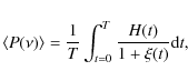
$\begin{displaymath}% \langle P(\nu)\rangle=\frac{1}{T}\int_{t=0}^T\frac{H(t)}{1+\xi(t)}{\rm d}t, \end{displaymath}$

(2)

where

$\begin{displaymath}% \xi(t)=\frac{2\left[\nu-\nu(t)\right]}{\Delta(t)}\cdot \end{displaymath}$

(3)

Here, H(t) is the instantaneous peak height of the profile, T is the total observing time, $\nu(t)$ is the frequency of the mode at time, t, and $\Delta(t)$ is the instantaneous width of the mode profile.

To determine the size of the frequency bias that occurs because of the distribution of activity levels we consider the simplistic case of a single mode whose peak height, H(t), and width, $\Delta(t)$ , remain constant with time. However, we take the peak frequency of the profile, $\nu(t)$ , to be a linear function of the activity at time, t.

For each day in the 8640-d time series we have produced a mode profile whose frequency was determined by the 10.7-cm radio flux observed on that day i.e. we use Eq. (1) to determine the frequency of the mode at time, t. We then summed the individual day Lorentzians to produce a single profile that was representative of the profile observed over a long time series. We found that the frequency of the final profile was not equal to the unweighted average of its time-varying frequency. Figure 3 shows the frequency correction applied to correct the observed frequency to the unweighted average frequency when H(t) and $\Delta(t)$ were constant. As can be seen the correction is significant and structured.

$\begin{figure} \par\includegraphics[height=4cm, clip]{12286fg3} \end{figure}$	Figure 3: Corrections applied to the 8640-d frequencies that occur due to the skewed distribution of the observed activity level i.e. the devil-in-the-detail corrections calculated when the mode heights and widths are kept constant with time.
Open with DEXTER

To understand this effect in more detail we consider the following ratio

$\begin{displaymath}% R=\frac{\delta\nu_{n,l}}{\Delta_{n,l}}, \end{displaymath}$

(4)

where $\delta\nu_{n,l}$ was determined using Eq. (1) for $\langle A(t)\rangle-\langle A(t)\rangle_{\rm c}=(118-64)~\rm RFU=54~\rm RFU$ . Figure 4 shows R plotted as a function of the mode frequency. Comparison with Fig. 3 shows that R has a similar structure to the observed frequency shift. Hence, the larger the shift experienced relative to the width of a mode the greater is the difference in the integrated profile frequency and the unweighted-mean frequency.

$\begin{figure} \par\includegraphics[height=4cm, clip]{12286fg4} \end{figure}$	Figure 4: Variation in R with mode frequency.
Open with DEXTER

In reality the above example is simplistic as the heights and widths of the mode profiles also vary with the solar cycle. To determine the size of the frequency shift due to both the distribution of the activity and the cross-talk between the cycle varying mode parameters we systematically altered the mode profile widths and heights with activity.

Between solar minimum and maximum mode widths are observed to increase by up to 17.5 per cent and mode heights are observed to decrease by twice this amount (Chaplin et al. 2000; Salabert et al. 2007). The variations in mode widths and heights are also functions of frequency. We have modelled the change in profile widths and heights in the manner shown in Fig. 5. Note that the size of the variation also depends linearly on the level of activity and the profiles shown in Fig. 5 represent the maximum changes in width and height respectively, which occur when the solar activity is at a maximum. We have varied the frequency of the mode in the same manner as before. We have then produced instantaneous profiles of a mode for each day in the 8640-d time series and we have used these profiles to produce an integrated profile which represents that observed in a long time series.

$\begin{figure} \par\mbox{\includegraphics[width=4.4cm, clip]{12286f5a}\includegraphics[width=4.4cm, clip]{12286f5b} }\end{figure}$	Figure 5: Left panel: model of how the percentage change in the mode profile width, $\Delta _{n,l}$ , changes with frequency. Right panel: model of how the percentage change in the mode profile height, H, changes with frequency. Both panels represent the maximum change expected and so are applicable when the activity level is at a maximum.
Open with DEXTER

The total devil-in-the-detail corrections applied to the 8640-d BiSON data are plotted in Fig. 6. These corrections include both the effect of the distribution of the activity level and the cross-talk between the variations in mode frequency, width, and height over the observation period. Comparison with Fig. 3 implies that the distribution of the activity level accounts for approximately half of the total devil-in-the-detail correction. The frequency corrections shown in Fig. 6 should be added to the observed frequencies, $\nu_{n,l}$ , to obtain frequencies that have been corrected for the devil-in-the-detail effect. For the 8640-d data set considered here the maximum devil-in-the-detail corrections are of the order of 5 times larger than the errors associated with the raw fitted frequencies.

$\begin{figure} \par\includegraphics[height=4cm, clip]{12286fg6} \end{figure}$	Figure 6: Devil-in-the-detail corrections that were used in Broomhall et al. (2009).
Open with DEXTER

4 Sun-as-a-star correction

Sun-as-a-star observations are taken from a perspective where the plane of the Sun's rotation axis is nearly perpendicular to the line-of-sight. Therefore, only modes where l+m is even have a non-negligible visibility in Sun-as-a-star observations. Furthermore, estimates of the centroid frequencies are dominated by the |m|=l components, which are the most prominent components observed in the multiplets. It can, therefore, be difficult to estimate the true centroid frequency of a mode.

The difference between the centroid and fitted frequencies depends on the level of activity over the period the observations were made. When the solar activity is at a minimum the components are observed to be in a near-symmetrical arrangement and so the fitted centroid frequency is close to the true centroid frequency. However, at moderate to high activity levels this is not the case as the mode components are not arranged symmetrically. Take, for example, an l=2 mode. The |m|=2 components will experience a larger shift at high activity levels than the m=0 component. The magnitude of observed asymmetry is related to the inhomogeneous distribution of the solar activity over the surface and the spherical harmonic associated with each visible m component. Therefore, the fitted frequencies differ from the true centroids by an amount that is dependent on l.

Appourchaux & Chaplin (2007) describe how to make a ``Sun-as-a-star'' correction, which is determined using the so called a coefficients that are found from fits for an unresolved Sun. The a coefficients were obtained from MDI data (Schou et al. 1998), which had the same activity levels as the BiSON data (Chaplin et al. 2004a). It is important to make this correction as the centroid frequency contains information on the spherically symmetric component of the internal structure and so is the required input for hydrostatic structure inversions. Furthermore, resolved solar observations are able to offer direct estimates of the centroid frequencies and so, to compare the frequencies determined using resolved and Sun-as-a-star data, the Sun-as-a-star correction should be employed.

Figure 7 shows the Sun-as-a-star corrections applied to the 8640-d BiSON data set. As can be seen, except for l=0 modes these corrections are similar in magnitude but opposite in sign to the devil-in-the-detail corrections. As the variation with frequency is different for the two different corrections it is still necessary to use both when examining the frequencies observed in long time series. The correction to the l=0 modes is zero as there is only one component to observe and by definition this is the centroid frequency.

$\begin{figure} \par\includegraphics[height=4cm, clip]{12286fg7} \end{figure}$	Figure 7: Sun-as-a-star corrections that were used in Broomhall et al. (2009).
Open with DEXTER

5 Summary

All three of the corrections described in this paper are dependent on the solar activity level over the period of the observations and so should be used when comparing the frequencies determined from data observed at different epochs. The linear solar cycle correction allows frequencies to be determined for a nominal activity level. The devil-in-the-detail correction accounts for the distribution of activity levels over the period of observations and the fact that mode profile heights, widths, and frequencies all vary with solar activity. This correction should be used when comparing frequencies obtained from data sets of different lengths, although the correction is only significant when the data sets are long. The Sun-as-a-star correction allows for the fact that only components where l+m is even can be detected in Sun-as-a-star data and should be used when comparing the frequencies obtained from resolved and Sun-as-a-star data. This is because, at times of high-activity, the m-components of a mode are not arranged symmetrically, and so, because not all components are visible, Sun-as-a-star observations measure a frequency that is slightly different to the centroid frequency.

Acknowledgements

We thank the anonymous referee for insightful comments. This paper utilises data collected by the Birmingham Solar-Oscillations Network (BiSON). We thank the members of the BiSON team, both past and present, for their technical and analytical support. We also thank P. Whitelock and P. Fourie at SAAO, the Carnegie Institution of Washington, the Australia Telescope National Facility (CSIRO), E. J. Rhodes (Mt. Wilson, Californa) and members (past and present) of the IAC, Tenerife. BiSON is funded by the Science and Technology Facilities Council (STFC).

References

Appourchaux, T., & Chaplin, W. J. 2007, A&A, 469, 1151 [NASA ADS] [CrossRef] [EDP Sciences] (In the text)
Broomhall, A.-M., Chaplin, W. J., Davies, G. R., et al. 2009, MNRAS, 396, L100 [NASA ADS] (In the text)
Chaplin, W. J., Elsworth, Y., Isaak, G. R., Miller, B. A., & New, R. 2000, MNRAS, 313, 32 [NASA ADS] [CrossRef]
Chaplin, W. J., Appourchaux, T., Elsworth, Y., et al. 2004a, A&A, 424, 713 [NASA ADS] [CrossRef] [EDP Sciences] (In the text)
Chaplin, W. J., Appourchaux, T., Elsworth, Y., et al. 2004b, A&A, 416, 341 [NASA ADS] [CrossRef] [EDP Sciences]
Chaplin, W. J., Elsworth, Y., Isaak, G. R., Miller, B. A., & New, R. 2004c, MNRAS, 352, 1102 [NASA ADS] [CrossRef] (In the text)
Chaplin, W. J., Elsworth, Y., Miller, B. A., Verner, G. A., & New, R. 2007, ApJ, 659, 1749 [NASA ADS] [CrossRef] (In the text)
Chaplin, W. J., Jiménez-Reyes, S. J., Eff-Darwich, A., Elsworth, Y., & New, R. 2008, MNRAS, 385, 1605 [NASA ADS] [CrossRef] (In the text)
Howe, R. 2008, Adv. Space Res., 41, 846 [NASA ADS] [CrossRef] (In the text)
Jain, K., Tripathy, S. C., & Hill, F. 2009, ApJ, 695, 1567 [NASA ADS] [CrossRef] (In the text)
Salabert, D., Chaplin, W. J., Elsworth, Y., New, R., & Verner, G. A. 2007, A&A, 463, 1181 [NASA ADS] [CrossRef] [EDP Sciences]
Schou, J., Antia, H. M., Basu, S., et al. 1998, ApJ, 505, 390 [NASA ADS] [CrossRef] (In the text)
Tapping, K. F., & Detracey, B. 1990, Sol. Phys., 127, 321 [NASA ADS] [CrossRef] (In the text)
Viereck, R., Puga, L., McMullin, D., et al. 2001, Geophys. Res. Lett., 28, 1343 [NASA ADS] [CrossRef] (In the text)

All Tables