| Issue |
A&A
Volume 502, Number 3, August II 2009
|
|
|---|---|---|
| Page(s) | 1043 - 1049 | |
| Section | Numerical methods and codes | |
| DOI | https://doi.org/10.1051/0004-6361/200810982 | |
| Published online | 15 June 2009 | |
Time-dependent radiative transfer with PHOENIX
D. Jack1 - P. H. Hauschildt1 - E. Baron1,2
1 - Hamburger Sternwarte, Gojenbergsweg 112, 21029 Hamburg, Germany
2 - Homer L. Dodge Department of Physics and Astronomy, University of Oklahoma, 440 W Brooks, Rm 100, Norman, OK 73019-2061, USA
Received 18 September 2008 / Accepted 3 April 2009
Abstract
Aims. We present first results and tests of a time-dependent extension to the general purpose model atmosphere code PHOENIX. We aim to produce light curves and spectra of hydro models for all types of supernovae.
Methods. We extend our model atmosphere code PHOENIX to solve time-dependent non-grey, NLTE, radiative transfer in a special relativistic framework. A simple hydrodynamics solver was implemented to keep track of the energy conservation of the atmosphere during free expansion.
Results. The correct operation of the new additions to PHOENIX were verified in test calculations.
Conclusions. We have shown the correct operation of our extension to time-dependent radiative transfer and will be able to calculate supernova light curves and spectra in future work.
Key words: stars: supernovae: general - radiative transfer - methods: numerical
1 Introduction
All types of supernovae are important for the role that they play in understanding stellar evolution and galactic nucleosynthesis and as cosmological probes. Type Ia supernovae are of particular cosmological interest, e.g., because the dark energy was discovered with type Ia supernovae (Perlmutter et al. 1999; Riess et al. 1998).
In dark energy studies, the goal now is to characterize the nature of the dark energy as a function of redshift. While there are other probes that will be used (gravitational lensing, baryon acoustic oscillations), a JDEM or Euclid mission will likely consider supernovae in some form. In planning for future dark energy studies both from space and from the ground, it is important to know whether the mission will require spectroscopy of modest resolution, or whether pure imaging or grism spectroscopy will be adequate. Several purely spectral indicators of peak luminosity have been proposed (Bongard et al. 2006; Nugent et al. 1995; Bronder et al. 2008; Le Du et al. 2009; Hachinger et al. 2006; Foley et al. 2008). What is required is an empirical and theoretical comparison of both light curve shape luminosity indicators (Pskovskii 1977; Phillips 1993; Goldhaber et al. 2001; Riess et al. 1996) and spectral indicators.
To make this comparison one needs to know more about the physics going on in a supernova explosion and to be able to calculate light curves and spectra self-consistently. Thus, we need to extend our code to time-dependent problems. While our primary focus is on type Ia supernovae, the time-dependent radiative transfer code is applicable to all types of supernovae, as well as to other objects, e.g., stellar pulsations.
In the following we present the methods we used to implement time dependence. First we focus on solving the energy equation (first law) and then turn our attention to time-dependent radiative transfer.
2 Equation of energy conservation
To compute light curves we extended PHOENIX with a time-dependent solution of the non-grey, NLTE radiative transfer problem in special relativistic environments and a simple hydrodynamic code to solve the free expanding case relevant to supernova light curves. The idea is to keep track of the conservation of energy for the gas and radiation together and to allow for different time scales for the gas and the radiation.
For the time-dependent radiative transfer problem we extended our
existing radiative transfer code PHOENIX (Hauschildt & Baron 2004b,1999).
The change in the energy density of a radiating material is given by
Eq. (96.15) in Mihalas & Mihalas (1984)
where E is the total energy density. All quantities are considered in the comoving frame. Pr is not the pressure, but rather mechanical power on the sphere of a radius r. Equation (1) is only valid to first order in v/c, and thus lacks the full special relativistic accuracy of PHOENIX. This is adequate for the velocities found in supernovae. The total energy density of a radiating fluid consists of the sum of the energy density of the material, the energy density of the radiation field, the kinetic energy density of the material, and the gravitational energy density:
 |
(2) |
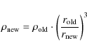
For supernovae in the free expansion phase, the gravitational energy density
With the assumption of homology, the velocity of a given matter
element is then constant as
is the kinetic energy
density. Thus, we can neglect the kinetic energy term
![]() .
So for our approach, we only have to consider the energy
densities of the radiation field and the material. For the material,
this includes effects such as an energy deposition due to radioactive
decay of nickel and cobalt in an SN Ia envelope.
.
So for our approach, we only have to consider the energy
densities of the radiation field and the material. For the material,
this includes effects such as an energy deposition due to radioactive
decay of nickel and cobalt in an SN Ia envelope.
The other possible cause of a change in the energy density is the
structure term. This term is given by (Cooperstein et al. 1986)
![\begin{displaymath}\frac{\partial}{\partial
M_{r}}\left(P_{r}+L_{r}\right)=\frac...
...ft\{4\pi
r^{2}\left[u\left(p+P_{0}\right)+F_{0}\right]\right\}
\end{displaymath}](/articles/aa/full_html/2009/30/aa10982-08/img6.png) |
(3) |
where p is the pressure of the material and P0the radiation pressure, u the velocity of the expanding gas, the radiative flux is represented by F0, and the mass inside of the radius r of a layer is given by Mr. The radiation pressure is a result of the solution of the detailed radiative transfer equation and given by
 |
(4) |
with K the second moment of the radiation field. The change of the energy density is given by the two quantities
| (5) |
and
 |
(6) |
If the atmosphere is in radiative equilibrium, the structure term is zero and the energy density stays constant if there is no additional energy source and the atmosphere is not expanding.
All the quantities required for the structure term can be derived from
thermodynamics or the solution of the radiative transfer problem. We
need the energy density of the material
![]() and the energy density of
the radiation field
and the energy density of
the radiation field
![]() .
For the latter, we have to
solve the radiative transfer equation for the radiation field and the
radiative energy. We use our radiative transfer code PHOENIX to solve
the time-independent radiative transfer equation.
The energy of the radiation field is given by
.
For the latter, we have to
solve the radiative transfer equation for the radiation field and the
radiative energy. We use our radiative transfer code PHOENIX to solve
the time-independent radiative transfer equation.
The energy of the radiation field is given by
 |
(7) |
where J is the mean intensity and c the speed of light.
The energy density of the material is given by
 |
(8) |
with the mean molecular weigh
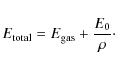
The change in this total energy density is given by Eq. (1). So the equation to calculate the new energy density
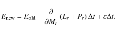
We now have all the needed equations to calculate a simple light curve. One problem for the calculation is that we can only determine the change in the total energy density for the next time step. However, the total energy change is divided into a change in the gas energy density and the energy density of the radiation field. To obtain the correct distribution of the gas and radiative energy, one has to iterate for each time step by solving the radiative transfer equation to compute the correct new temperature at the next time step.
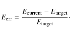
To get the correct new temperature we apply the following
iteration scheme.
The error in the energy density,
![]() is given by
is given by
 |
(11) |
Here,
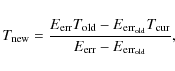 |
(12) |
where
3 Test light curves
For the first test calculations we have solved the radiative transfer equation for a grey test atmosphere. Test model atmospheres are divided in 100 layers and we consider here time independent radiative transfer (in Sect. 4 below we discuss time dependent radiative transfer).
As a first test we applied our time evolution code to a static atmosphere. The test atmosphere is not expanding and no energy sources are present. Inside the test atmosphere we used a ``lightbulb'' radiating with a constant luminosity to simulate the internal energy flow from a star. We assumed an approximate temperature structure for t=0 and then let the atmosphere evolve towards radiative equilibrium. The atmosphere changed until it reaches steady state and the luminosity is constant in both space and time. The resulting final temperature structure should be identical to the structure for radiative equilibrium computed directly.
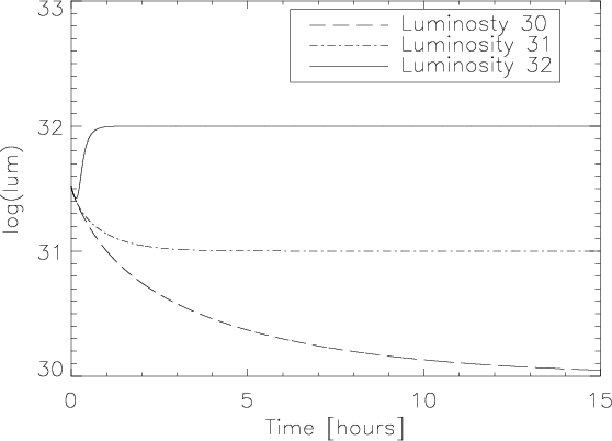 |
Figure 1: Three different light curves for the evolution to a stationary state. The three models have different luminosities produced by differentinner ``lightbulbs''. |
| Open with DEXTER | |
In Fig. 1 we show the light curves for three different static models. We can observe the model on its way towards radiative equilibrium. All calculations were started from the same temperature structure. After a certain time, the radiative relaxation time scale, each atmosphere has the (constant) luminosity of the lightbulb throughout the configuration.
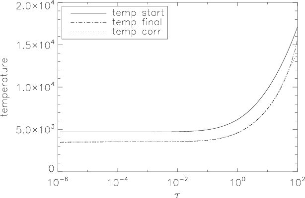 |
Figure 2: The final temperature structures of the time evolution calculations. |
| Open with DEXTER | |
The final temperature structure of the model atmosphere with the lightbulb with a luminosity of 1031 erg/s is displayed in Fig. 2. Also shown is the result of a calculation using the temperature correction procedure of PHOENIX (Hauschildt et al. 2003) to directly compute the radiative equilibrium structure of the configuration. As one can clearly see, the resulting temperature structure of both methods agrees very well, and the maximum deviation of the temperature structure is less than one percent. Only the inner three layers have a deviation of up to 10 percent due to the implicit assumption of a diffusion approximation (and not a lightbulb) in the static calculation.
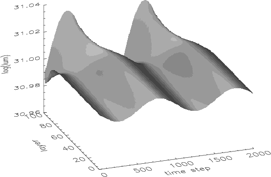 |
Figure 3: The flux in every layer at each time step. |
| Open with DEXTER | |
The next test is to look at time varying atmospheres. As an example we considered an atmosphere with a sinusoidally varying lightbulb inside. The resulting luminosity in each layer at each time point is plotted in Fig. 3. The luminosity in each layer is sinusoidal. It takes some time for the radiation to reach the outside boundary of the atmosphere and this results in a phase shift compared to the lightbulb.
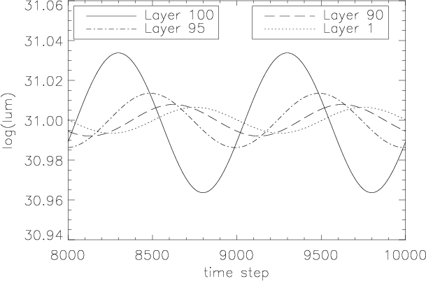 |
Figure 4:
The result for a sinusoidal varying lightbulb.
Shown here is the luminosity in different layers. The phase
shift between the lightbulb and the emergent flux is roughly |
| Open with DEXTER | |
We now take a look at the luminosity in different layers. These are plotted in Fig. 4. One can see the phase shift of the sine in each layer. As expected, the luminosity from the central source needs time to move through the atmosphere.
One can also see that the amplitude of the sine decreases with increasing radius. What one would expect is that the amplitude is the same in every layer. The radiation is moving outwards and the incoming varying luminosity from the lightbulb should move through every layer and therefore the amplitude is supposed to be the same in each layer. If we integrate the luminosity over a whole sine, it stays constant in every layer. In the plot one can see that the mean luminosity is at the same level, so the luminosity is preserved. But why does the amplitude decrease? A possible explanation is that the radiation moving through the atmosphere is going backwards when the sine is declining, so this smears out the amplitude. If the sine varying radiation is moving through a very thick atmosphere, the amplitude at the top of the atmosphere is finally flat. An observer sees the mean luminosity.
For the next test we consider an atmosphere with an internal energy source. The initial structure is the radiative equilibrium structure of the static model with the lightbulb with a luminosity of 1031 erg/s. We assume a constant energy deposition rate in each layer of the model atmosphere. The luminosity is expected to increase over time and towards the outside. Figure 5 shows a plot of the light curve of this test atmosphere. The luminosity increases in time because of the energy deposition.
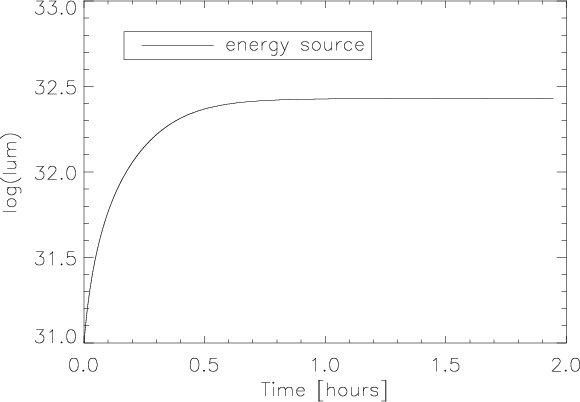 |
Figure 5: The light curve of an lightbulb with an additional energy source. An energy source in each layer causes an increasing luminosity of the model atmosphere. |
| Open with DEXTER | |
3.1 Expansion
In the case of SN Ia, homologous expansion is a good assumption after
the initial breakout. In our test model each layer has a
constant velocity,
![]() ,
to simulate a freely expanding
envelope. The new radius
,
to simulate a freely expanding
envelope. The new radius
![]() of a layer is, therefore,
determined by
of a layer is, therefore,
determined by
| (13) |
for a time step
 |
(14) |
where
| (15) |
where p is the pressure and
 |
(16) |
The mass m of a layer is given by its volume and density
| (17) |
In our approach to a homologous expanding supernova of the type Ia, we consider each layer has a constant mass, so the derivative
 |
(18) |
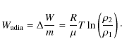
Together with the equation of state
 |
(19) |
we obtain the work for the adiabatic expansion as
 |
(20) |
For differences in a time step
 |
(21) |
For the first test of a light curve for a supernova with an expanding atmosphere, we neglect the interaction between the layers, meaning the structure term is equal to the work of the adiabatic expansion so that
 |
(22) |
As we now consider expanding atmospheres, we use more supernova-like structures for the tests. We set the maximum velocity to 30 000 km s-1and use a radius of
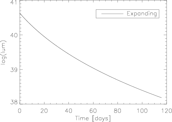 |
Figure 6: Light curve of an atmosphere that is just expanding. |
| Open with DEXTER | |
Figure 6 shows a plot of the light curve of supernova test atmosphere that is simply expanding. We considered time-independent radiative transfer and a grey atmosphere. As one can see, the luminosity is decreasing, because the atmosphere is cooling down adiabatically.
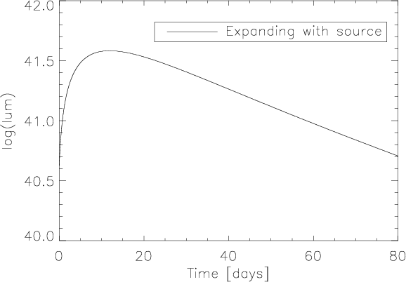 |
Figure 7: Light curve of an atmosphere that is expanding and has an energy source. It has the typical shape of a light curve of a SN Ia. The luminosity rises due to the energy deposition. After the maximum we see the decline resulting from the expansion. |
| Open with DEXTER | |
Now we test a setup more closely resembling a real supernova light curve. Therefore, we take an initial atmosphere structure and add an energy source (radioactive decay) in each layer. The energy source exponentially decreases to simulate declining activity of the radioactive species. Figure 7 shows the plot of the light curve of this test, resulting in a light curve with a supernova-like shape. We have a rising part of the light curve at the beginning because of the energy deposition. After the maximum, the luminosity decreases due to the ongoing expansion and decreasing energy deposition. Of course this light curve is far from correct because the assumption of a grey atmosphere is a bad assumption for an SN Ia. But the tests show that the code behaves as expected.
3.2 Entropy
We calculated the entropy to test the code. Because energy is moving through the atmosphere, entropy is not conserved. Nevertheless, testing entropy conservation is an important test of the correctness of the code. Therefore, we calculated the entropy change in the case of pure adiabatic expansion. For testing, we neglected interaction between layers and gamma ray deposition and calculated the entropy change for a time step for the just expanding case.
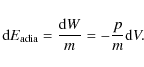
To be consistent with our hydrodynamics equations, we deduced the entropy from the first law of
thermodynamics.
A change in the entropy during a time step is therefore
given by
 |
(23) |
where 2 is the index of quantities at the new time and 1 the one of the old. For the integration of the temperature and the density term, we kept
The entropy given here is only the entropy of the gas, so to check that the expansion worked right we had to neglect the radiation energy density in our energy density conservation equation. Furthermore we ignored the interaction between the layers and neglected the structure term. We now have only a change in the energy due to the adiabatic expansion.
With this setup we calculated a few time steps and checked the
entropy. Even for a long time step of 1000 s the entropy stays almost constant.
The relative change of the entropy was ![]() 10-6.
10-6.
4 Time-dependent radiative transfer
So far, our radiative transfer code only solves the time-independent
radiative transfer equation. For an implementation of the time
dependence in the radiative transfer itself, the spherical symmetric
special relativistic radiative transfer equation (SSRTE) for expanding
atmospheres (Hauschildt & Baron 1999) is extended so that the additional time
dependent term is given by
 |
(24) |
where
 |
(25) |
where
 |
(26) |
Along the characteristics the equation has the form
 |
(27) |
where
4.1 Discretization of the time derivative
We used the first discretization as described in Hauschildt & Baron (2004a) and added
the time dependent term. We discretized the time-dependent, as well as
the wavelength, derivative in the SSRTE with an fully implicit method.
The discretization of the time dependent term is given by
 |
(28) |
so the SSRTE including the time discretization can be written as
 |
(29) |
where I is the intensity at wavelength point
 |
(30) |
Introducing the source function
 |
(31) |
We now have a modification of the source function and a new definition of the optical depth scale along a ray. With this redefinition of the optical depth and the source function, one can now proceed with the formal solution as described in Hauschildt & Baron (2004a).
4.2 Test calculations: time-dependent radiative transfer
For the test of the time-dependent radiative transfer, we used a static atmosphere structure to see the direct effects of the time dependence of the radiative transfer. Therefore, the temperature, radius, and density are all constant in time. For the test we then changed the inner boundary condition for the radiation (the ``lightbulb'') to initiate a perturbation of the radiation field, which then moves through the atmosphere via the time-dependent radiation transfer.
For the first test we switched on an additional light source inside the atmosphere. This light source has a luminosity of 109 times higher then the inner lightbulb.
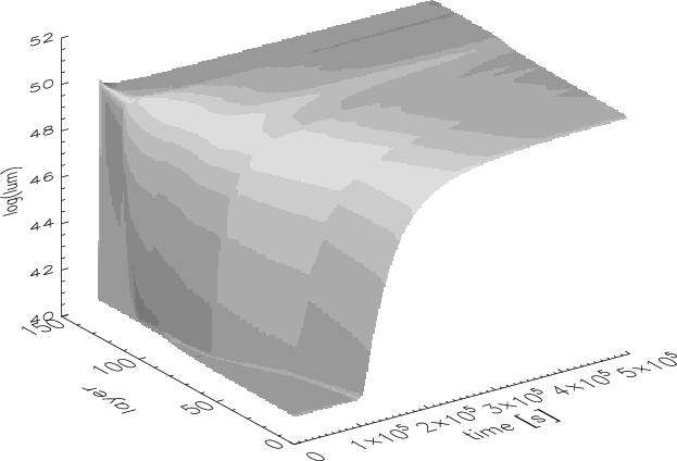 |
Figure 8: Luminosity of each layer and time step of our test atmosphere. |
| Open with DEXTER | |
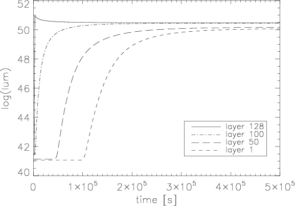 |
Figure 9: The light curves of a few layers. In this case the atmosphere has an additional light source switching on inside. The radiation needs time to get to the outer layers. |
| Open with DEXTER | |
We compared our time scale to the radiation diffusion time scale.
Assuming a random-walk process the mean free path for a photon is given by
![]() ,
where
,
where
![]() is the mean opacity.
For a travel distance l the time
is the mean opacity.
For a travel distance l the time ![]() a photon needs is given by
a photon needs is given by
 |
(32) |
where c is the speed of light. For the mean opacity
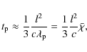
An important test is also to check that the results of the time-dependent radiative transfer calculation depend on the size of the time step. We tested this with a model that has a small perturbation inside that is moving outwards. This was calculated with two different time steps. In Fig. 10 the results of calculations with two different time steps are shown. As one can see, the result does not depend on the size of the time step.
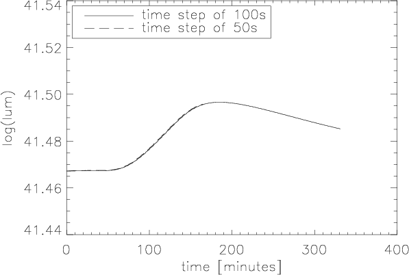 |
Figure 10: The light curve of an atmosphere where a small perturbation moves outwards. The two plotted light curves of layer 110 were calculated with different time steps. |
| Open with DEXTER | |
In the next test we put a sinusoidally varying light bulb inside of our test atmosphere. In Fig. 11, we show a plot of the luminosity for each time step. After a while, the luminosity of the whole atmosphere varies sinusoidally and steady state is reached.
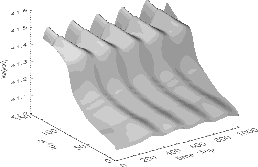 |
Figure 11: Luminosity in each layer and time step. The light source inside the atmosphere varies sinusoidally. |
| Open with DEXTER | |
5 Conclusion
We have implemented a time evolution code into our general-purpose model atmosphere code PHOENIX, which keeps track of the energy conservation. Because a homologous expansion is a good assumption for supernovae in general and particularly for type Ia supernovae, we considered adiabatic free expansion for our code. With first test calculations, we reproduced the expected behavior of the test cases. Static atmospheres adopted the luminosity of an internal lightbulb and perturbations of the lightbulb moved outwards in time. We also calculated a light curve that had the shape of a typical supernovae Ia light curve.
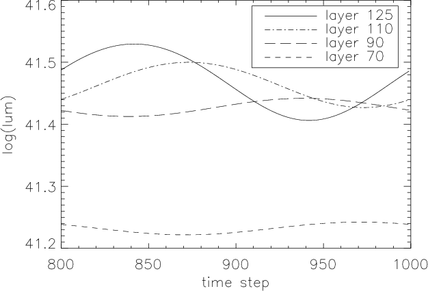 |
Figure 12: Flux at different radii of a sinusoidally varying atmosphere. |
| Open with DEXTER | |
To complete the physics of time-dependent processes in a supernova
atmosphere, we extended our code even further. PHOENIX now solves the time
dependent radiative transfer equation. We presented the new
discretization scheme of the time dependent
![]() term. We checked our code with a series of tests. A
perturbation can be followed on its way through the atmosphere. We
ran a test model with a sinusoidal source. In steady state the whole
atmosphere was varying sinusoidally, responding to the source.
A phase shift between the inner and outer
layers could also be observed. All tests indicate that our extended
code works fine.
term. We checked our code with a series of tests. A
perturbation can be followed on its way through the atmosphere. We
ran a test model with a sinusoidal source. In steady state the whole
atmosphere was varying sinusoidally, responding to the source.
A phase shift between the inner and outer
layers could also be observed. All tests indicate that our extended
code works fine.
Future work is to calculate realistic light curves for type Ia supernova hydro models. As a first step we can consider the atmosphere to be in LTE, but including detailed opacities and treating full line blanketing.
Also with our time-dependent radiative transfer, we can address a longstanding debate about the importance of time dependence in calculating the spectra of type Ia supernovae (Eastman & Pinto 1993; Baron et al. 1996). One challenge is the computation time needed for a whole light curve with more complex NLTE radiative transfer.
Acknowledgements
This work was supported in part by the Deutsche Forschungsgemeinschaft (DFG) via the SFB 676, NASA grant NAG5-12127, NSF grant AST-0707704, and US DOE Grant DE-FG02-07ER41517. This research used resources of the National Energy Research Scientific Computing Center (NERSC), which is supported by the Office of Science of the U.S. Department of Energy under Contract No. DE-AC02-05CH11231, and the Höchstleistungs Rechenzentrum Nord (HLRN). We thank all these institutions for generous allocations of computer time.
References
- Baron, E., Hauschildt, P. H., & Mezzacappa, A. 1996, MNRAS, 278, 763 [NASA ADS]
- Bongard, S., Baron, E., Smadja, G., Branch, D., & Hauschildt, P. 2006, ApJ, 647, 480 [NASA ADS] [CrossRef]
- Bronder, T. J., Hook, I. M., Astier, P., et al. 2008, A&A, 477, 717 [NASA ADS] [CrossRef] [EDP Sciences]
- Cooperstein, J., van den Horn, L. J., & Baron, E. 1986, ApJ, 309, 653 [NASA ADS] [CrossRef] (In the text)
- Eastman, R., & Pinto, P. 1993, ApJ, 412, 731 [NASA ADS] [CrossRef]
- Foley, R. J., Filippenko, A. V., & Jha, S. W. 2008, A&A [ArXiv:0803.1181]
- Goldhaber, G., Groom, D. E., Kim, A., et al. 2001, ApJ, 558, 359 [NASA ADS] [CrossRef]
- Hachinger, S., Mazzali, P. A., & Benetti, S. 2006, MNRAS, 370, 299 [NASA ADS]
- Hauschildt, P. H., & Baron, E. 1999, J. Comp. Appl. Math., 109, 41 [NASA ADS] [CrossRef]
- Hauschildt, P. H., & Baron, E. 2004a, A&A, 417, 317 [NASA ADS] [CrossRef] [EDP Sciences] (In the text)
- Hauschildt, P. H., & Baron, E. 2004b, Mitteilungen der Mathematischen Gesellschaft in Hamburg, 24, 1
- Hauschildt, P. H., Barman, T. S., Baron, E., & Allard, F. 2003, in Stellar Atmospheric Modeling, ed. I. Hubeny, D. Mihalas, & K. Werner (San Francisco: ASP), 227 (In the text)
- Le Du, J., et al. 2009, preprint
- Mihalas, D., & Mihalas, B. W. 1984, Foundations of Radiation Hydrodynamics (Oxford: Oxford University) (In the text)
- Nugent, P., Phillips, M., Baron, E., Branch, D., & Hauschildt, P. 1995, ApJ, 455, L147 [NASA ADS] [CrossRef]
- Perlmutter, S., Aldering, G., Goldhaber, G., et al. 1999, ApJ, 517, 565 [NASA ADS] [CrossRef]
- Phillips, M. M. 1993, ApJ, 413, L105 [NASA ADS] [CrossRef]
- Pinto, P. A., & Eastman, R. G. 2000, ApJ, 530, 744 [NASA ADS] [CrossRef] (In the text)
- Pskovskii, I. P. 1977, Sov. Astron., 21, 675 [NASA ADS]
- Riess, A., Filippenko, A. V., Challis, P., et al. 1998, AJ, 116, 1009 [NASA ADS] [CrossRef]
- Riess, A. G., Press, W. H., & Kirshner, R. P. 1996, ApJ, 473, 88 [NASA ADS] [CrossRef]
- Woosley, S. E., Kasen, D., Blinnikov, S., & Sorokina, E. 2007, ApJ, 662, 487 [NASA ADS] [CrossRef] (In the text)
All Figures
| |
Figure 1: Three different light curves for the evolution to a stationary state. The three models have different luminosities produced by differentinner ``lightbulbs''. |
| Open with DEXTER | |
| In the text | |
| |
Figure 2: The final temperature structures of the time evolution calculations. |
| Open with DEXTER | |
| In the text | |
| |
Figure 3: The flux in every layer at each time step. |
| Open with DEXTER | |
| In the text | |
| |
Figure 4:
The result for a sinusoidal varying lightbulb.
Shown here is the luminosity in different layers. The phase
shift between the lightbulb and the emergent flux is roughly |
| Open with DEXTER | |
| In the text | |
| |
Figure 5: The light curve of an lightbulb with an additional energy source. An energy source in each layer causes an increasing luminosity of the model atmosphere. |
| Open with DEXTER | |
| In the text | |
| |
Figure 6: Light curve of an atmosphere that is just expanding. |
| Open with DEXTER | |
| In the text | |
| |
Figure 7: Light curve of an atmosphere that is expanding and has an energy source. It has the typical shape of a light curve of a SN Ia. The luminosity rises due to the energy deposition. After the maximum we see the decline resulting from the expansion. |
| Open with DEXTER | |
| In the text | |
| |
Figure 8: Luminosity of each layer and time step of our test atmosphere. |
| Open with DEXTER | |
| In the text | |
| |
Figure 9: The light curves of a few layers. In this case the atmosphere has an additional light source switching on inside. The radiation needs time to get to the outer layers. |
| Open with DEXTER | |
| In the text | |
| |
Figure 10: The light curve of an atmosphere where a small perturbation moves outwards. The two plotted light curves of layer 110 were calculated with different time steps. |
| Open with DEXTER | |
| In the text | |
| |
Figure 11: Luminosity in each layer and time step. The light source inside the atmosphere varies sinusoidally. |
| Open with DEXTER | |
| In the text | |
| |
Figure 12: Flux at different radii of a sinusoidally varying atmosphere. |
| Open with DEXTER | |
| In the text | |
Copyright ESO 2009
Current usage metrics show cumulative count of Article Views (full-text article views including HTML views, PDF and ePub downloads, according to the available data) and Abstracts Views on Vision4Press platform.
Data correspond to usage on the plateform after 2015. The current usage metrics is available 48-96 hours after online publication and is updated daily on week days.
Initial download of the metrics may take a while.