| Issue |
A&A
Volume 502, Number 1, July IV 2009
|
|
|---|---|---|
| Page(s) | 189 - 197 | |
| Section | Interstellar and circumstellar matter | |
| DOI | https://doi.org/10.1051/0004-6361/200912076 | |
| Published online | 27 May 2009 | |
Abundances in planetary nebulae: NGC 2792![[*]](/icons/foot_motif.png)
S. R. Pottasch1 - R. Surendiranath2 - J. Bernard-Salas3 - T. L. Roellig4
1 - Kapteyn Astronomical Institute, P.O. Box 800, NL 9700 AV Groningen, The Netherlands
2 -
Indian Institute of Astrophysics, Koramangala II Block, Bangalore-560034, India
3 -
Center for Radiophysics and Space Research, Cornell University, Ithaca, NY 14853, USA
4 -
NASA Ames Research Center, MS 245-6, Moffett Field, CA 94035-1000, USA
Received 16 March 2009 / Accepted 15 May 2009
Abstract
The mid-infrared spectrum of the rather circular planetary
nebula NGC 2792 taken with the Spitzer Space
Telescope is presented. This spectrum is combined with the
ultraviolet IUE spectrum and with the spectrum in the visual
wavelength region to obtain a complete, extinction corrected,
spectrum. The chemical composition of the nebula is then
calculated in two ways. First by directly calculating and adding
individual ion abundances, and secondly by building a model nebula
that attempts to reproduce the observed spectrum. Because it is now
possible to include the nebular temperature gradient, the chemical
composition is more accurate than has been given
earlier in the literature. Discussion of both the central star and
the evolution of the star-nebula is then given.
Key words: ISM: abundances - planetary nebulae: individual: NGC 2792 - infrared: ISM - ISM: lines and bands
1 Introduction
NGC 2792 (PK 265.7+04.1) is a rather average planetary nebula. An image
in visible light is shown as Fig. 1. The nebula is usually classified
as elliptical although it is almost circular in shape. In addition it
contains several structural details. A halo is present as
has been measured by Corradi et al. (2003). These authors
measure a radius of 5.5
![]() for the bright inner part of the
nebula, which is surrounded by a fainter nebula which decreases in
brightness to about a radius of 10
for the bright inner part of the
nebula, which is surrounded by a fainter nebula which decreases in
brightness to about a radius of 10
![]() .
The halo continues at a
very low surface brightness (less than 10-3 of the brightness of
the main nebula) until a radius of about 37
.
The halo continues at a
very low surface brightness (less than 10-3 of the brightness of
the main nebula) until a radius of about 37
![]() .
.
![\begin{figure}
\par\includegraphics[width=8.4cm,height=9cm]{fig1.ps}
\end{figure}](/articles/aa/full_html/2009/28/aa12076-09/img5.png) |
Figure 1: HST image of NGC 2792; Credits: Howard Bond; HST archived exposures catalog (STSCI, 2007). |
| Open with DEXTER | |
The distance of the nebula is very uncertain. Statistical distances
are between 1.4 kpc and 3 kpc. By equating the
![]() density with
the forbidden line density, a value of d=1.5 kpc is found and used
when necessary throughout this paper. This distance is close to the
value of 1.9 kpc found by the extinction method by Gathier et al. (1986). Adopting this value, the nebula is thus about 100 pc above
the galactic plane.
density with
the forbidden line density, a value of d=1.5 kpc is found and used
when necessary throughout this paper. This distance is close to the
value of 1.9 kpc found by the extinction method by Gathier et al. (1986). Adopting this value, the nebula is thus about 100 pc above
the galactic plane.
The purpose of this paper is to obtain accurate abundances for this nebula. This is achieved in two ways. First by including the mid-infrared spectrum taken with the IRS spectrograph of the Spitzer Space Telescope (Werner et al. 2004). The reasons for this have been discussed in earlier papers (e.g. see Pottasch & Beintema 1999; Pottasch et al. 2000, 2001; Bernard Salas et al. 2001), and can be summarized as follows: 1) the intensity of the infrared lines is not very sensitive to the electron temperature nor to possible extinction effects; 2) use of the infrared line intensities enable a more accurate determination of the electron temperature for use with the visual and ultraviolet lines; 3) the number of observed ionization stages is doubled.
The second method of improving the abundances is by using a nebular model to determine them. This has several advantages. First it provides a physical basis for the electron temperature determination. Secondly it permits abundance determination for elements which are observed in only one, or a limited number of ionic stages. This is true of Mg, Si, and Cl, which would be less reliably determined without a model. A further advantage of modeling is that it provides information on the central star and other properties of the nebula.
A disadvantage of modeling is that there are more unknowns than observations and some assumptions must be made; for example, concerning the geometry, we will assume that the nebula is spherical and that no clumping exists. The observed circular form and smooth emission make these assumptions reasonable. Furthermore we are limited in the form of the radiation field of the exciting star. Other assumptions are discussed in Sect. 4.1.
Abundance determination for this nebula has been made earlier. The most extensive are the works of Milingo et al. (2002a,b; see also Henry et al. 2005), and Kingsburgh & Barlow (1994). A more limited number of elements have been studied by Torres-Peimbert & Peimbert (1977) and by de Freitas Pacheco et al. (1992). These authors give differing and incomplete abundance values; our purpose is to bring order in this situation.
This paper is structured as follows. First the spectrum of NGC 2792 is discussed (in Sect. 2). Section 3 discusses the simple approach to determining the chemical composition and presents the resultant abundances. In Sect. 4. the model assumptions are detailed and the results are presented. The results of the model are discussed in detail in Sect. 5. The abundances determined are compared with those in the literature in Sect. 6, which also includes a discussion of the errors. In Sect. 7 a discussion of the central star and the evolutionary state of the nebula is given. Finally, our conclusions are given in Sect. 8.
2 The spectrum of NGC 2792
2.1 The infrared spectrum
Observations of NGC 2792 were made using the Infrared Spectrograph (IRS, Houck et al. 2004) on board the Spitzer Space Telescope with AOR keys of 4111104 (on target) and 4111360 (background). The reduction started from the droop images which are equivalent to the most commonly used Basic Calibrated Data (bcd) images but lack stray-cross removal and flat-field. The data were processed using the s15.3 version of the pipeline and using a script version of Smart (Higdon et al. 2004). The tool irsclean was used to remove rogue pixels. The different cycles for a given module were combined to enhance the S/N. At this point the background images were subtracted to remove the sky contribution. We note that since we are interested in line fluxes the removal of background is irrelevant for our analysis except for aiding in the removal of any rogue pixel that may have been left out by the irsclean tool (i.e. those with low flux). Then the resulting high-resolution modules (HR) were extracted using full aperture measurements.
The IRS high resolution spectra have a spectral resolution of about 600, which is a factor of between 2 and 5 less than the resolution of the ISO SWS spectra. The mid-infrared measurements are made with several different diaphragm sizes. Because the diaphragms are smaller than the size of the nebulae and are all of differing size, we first discuss how the different spectra are placed on a common scale.
![\begin{figure}
\par\includegraphics[width=6.3cm,angle=90]{plot_n2792.eps}
\end{figure}](/articles/aa/full_html/2009/28/aa12076-09/img7.png) |
Figure 2:
The IRS spectrum of NGC/,2792. The SH intensity (from 9.9 |
| Open with DEXTER | |
Two of the three diaphragms used have high resolution: the short high module
(SH) measures from 9.9 ![]() m to
19.6
m to
19.6 ![]() m and the long high module (LH) from 18.7
m and the long high module (LH) from 18.7 ![]() m to
37.2
m to
37.2 ![]() m. The SH has a diaphragm size of 4.7
m. The SH has a diaphragm size of 4.7
![]()
![]() 11.3
11.3
![]() ,
while the LH is 11.1
,
while the LH is 11.1
![]()
![]() 22.3
22.3
![]() .
If the nebulae are
uniformly illuminating then the ratio of the intensities would
simply be the ratio of the areas measured by the two diaphragms.
Since this is not so, we may use the ratio of the continuum intensity
in the region of wavelength overlap at 19
.
If the nebulae are
uniformly illuminating then the ratio of the intensities would
simply be the ratio of the areas measured by the two diaphragms.
Since this is not so, we may use the ratio of the continuum intensity
in the region of wavelength overlap at 19 ![]() m. These continua are equal
when the SH intensities are increased by a factor of 2.65. The third
diaphragm is a long slit which is
4
m. These continua are equal
when the SH intensities are increased by a factor of 2.65. The third
diaphragm is a long slit which is
4
![]() wide and extends over the entire nebula. This SL module measures in
low resolution and measures between 5.5
wide and extends over the entire nebula. This SL module measures in
low resolution and measures between 5.5 ![]() m and 14
m and 14 ![]() m. These spectra
are normalized by making the lines in common between the SL and SH
modules to agree. Especially important is the agreement of the
[S IV] line at 10.51
m. These spectra
are normalized by making the lines in common between the SL and SH
modules to agree. Especially important is the agreement of the
[S IV] line at 10.51 ![]() m. The spectrum is shown in Fig. 2.
m. The spectrum is shown in Fig. 2.
The IRS measurement of NGC 2792 was centered at RA(2000)
09![]() 12
12![]() 26.63
26.63![]() and Dec(2000)
-42°25
and Dec(2000)
-42°25![]() 40.1
40.1
![]() .
This is almost exactly the same as the
value measured by Kerber et al. (2003) of RA(2000)
09
.
This is almost exactly the same as the
value measured by Kerber et al. (2003) of RA(2000)
09![]() 12
12![]() 26.60
26.60![]() and Dec(2000)
-42°25
and Dec(2000)
-42°25![]() 39.9
39.9
![]() ,
which is presumably the coordinate of
the central star. Thus the IRS measurement was well centered on the
nebula. The fluxes were measured using the Gaussian
line-fitting routine. The measured emission line intensities are given in
Table 1, after correcting the SH measurements by the factor 2.65 and the SL
measurements by a factor of 5.5, in the
column labeled ``intensity''. The H
,
which is presumably the coordinate of
the central star. Thus the IRS measurement was well centered on the
nebula. The fluxes were measured using the Gaussian
line-fitting routine. The measured emission line intensities are given in
Table 1, after correcting the SH measurements by the factor 2.65 and the SL
measurements by a factor of 5.5, in the
column labeled ``intensity''. The H![]() flux found from the infrared
hydrogen lines (especially the lines at 12.37
flux found from the infrared
hydrogen lines (especially the lines at 12.37 ![]() m) using the theoretical
ratios of Hummer & Storey (1987),
is
m) using the theoretical
ratios of Hummer & Storey (1987),
is
![]() erg cm-2 s-1, which is about 95% of the total
H
erg cm-2 s-1, which is about 95% of the total
H![]() intensity. This is reasonable since the well-centered LH diaphragm
coves much of the nebula.
intensity. This is reasonable since the well-centered LH diaphragm
coves much of the nebula.
Table 1: IRS spectrum of NGC 2792.
2.2 The visual spectrum
The visual spectrum has been measured by four authors. We list here the results. The line intensities listed have been corrected by each author for a value of extinction determined by them to obtain a theoretically correct Balmer decrement. The results are listed in Table 2, where the last column lists the average value which we have used. No attempt has been made to use a common extinction correction because then the Balmer decrement will be incorrect. The value of extinction C which the individual authors found is listed at the bottom of the table. None of the spectra measure the weaker lines very well. The errors may be judged by the agreement (or disagreement) of the various measures and appear to be within 20% for the stronger lines and probably much worse for the weaker lines.
2.3 The IUE ultraviolet spectrum
Only three IUE observations of NGC 2792 were made. Two were
short-wavelength measurements, SWP16018 and SWP16032, and a
long-wavelength measurement, LWR12326. All of them were made at the
position RA(2000) 09![]() 12
12![]() 26.74
26.74![]() and Dec(2000)
-42°25
and Dec(2000)
-42°25![]() 31.6
31.6
![]() ,
which is about 8
,
which is about 8
![]() from the center
of the nebula, so that only part of the nebula was seen. In order to
account for the missing radiation and for the extinction a
correction was made in the
short-wavelength region by assuming a theoretical ratio for
the He II line ratio
from the center
of the nebula, so that only part of the nebula was seen. In order to
account for the missing radiation and for the extinction a
correction was made in the
short-wavelength region by assuming a theoretical ratio for
the He II line ratio ![]() 1640/
1640/![]() 4686 Å at
T=15 000 K and an
4686 Å at
T=15 000 K and an ![]() of 103 cm-3. The ratio of
of 103 cm-3. The ratio of
![]() 1640 to H
1640 to H![]() can then be found using the
can then be found using the
![]() 4686/H
4686/H![]() ratio in Table 2. A further correction for
extinction relative to
ratio in Table 2. A further correction for
extinction relative to ![]() 1640 Å is then made using the
reddening curve of Fluks et al. (1994) and a value of the
extinction constant C=0.80 (see below). For the long-wavelength
region essentially the same procedure was carried out, the only
difference being that an average value for the He II lines at
1640 Å is then made using the
reddening curve of Fluks et al. (1994) and a value of the
extinction constant C=0.80 (see below). For the long-wavelength
region essentially the same procedure was carried out, the only
difference being that an average value for the He II lines at
![]() 2733 Å and
2733 Å and ![]() 3204 Å were used. This has the
consequence that the correction for diaphragm size is somewhat
different in the two wavelength regions, probably because the actual
position of the measurements were slightly different. The value of
the intensity of the C III
3204 Å were used. This has the
consequence that the correction for diaphragm size is somewhat
different in the two wavelength regions, probably because the actual
position of the measurements were slightly different. The value of
the intensity of the C III ![]() 1906 Å line, which was
measured in both wavelength regions, is found to have the same ratio
with respect to H
1906 Å line, which was
measured in both wavelength regions, is found to have the same ratio
with respect to H![]() in both regions. The uncertainties in the
intensities are estimated to be 30% for the stronger lines and 50%
for the weaker lines. The results are shown in the last two columns
of Table 3, where the measured intensities are given in Col. 3, the
intensities corrected for diaphragm size and for extinction are found
in Col. 4, and the last column gives the ratio of the intensity to
H
in both regions. The uncertainties in the
intensities are estimated to be 30% for the stronger lines and 50%
for the weaker lines. The results are shown in the last two columns
of Table 3, where the measured intensities are given in Col. 3, the
intensities corrected for diaphragm size and for extinction are found
in Col. 4, and the last column gives the ratio of the intensity to
H![]() ,
normalized to
,
normalized to
![]() .
.
Table 2: Visual spectrum of NGC 2792.
Table 3: IUE spectrum of NGC 2792.
![\begin{figure}
\par\includegraphics[width=9cm,clip]{fig2.ps}
\end{figure}](/articles/aa/full_html/2009/28/aa12076-09/img19.png) |
Figure 3: The input density profile. The ordinate is the electron density. |
| Open with DEXTER | |
2.4 Extinction
The two methods which can be used for obtaining the extinction are:
(1) comparison of radio emission with H![]() flux, and (2)
comparison of observed and theoretical Balmer decrement. The four
values of the extinction correction C(H
flux, and (2)
comparison of observed and theoretical Balmer decrement. The four
values of the extinction correction C(H![]() )
which are found in the
literature are given in Table 2, and are seen to have a rather large
range. Let us discuss the radio emission and the H
)
which are found in the
literature are given in Table 2, and are seen to have a rather large
range. Let us discuss the radio emission and the H![]() flux.
flux.
2.4.1 The 6 cm radio emission and the H flux
flux
The 6 cm flux density has been measured by Gregory et al. (1994) as 127 mJy and by Wright et al.
(1994) as 139 mJy. We use an average value of 133 mJy.
This implies an H![]() flux of
flux of
![]() erg cm-2 s-1. Given an observed H
erg cm-2 s-1. Given an observed H![]() flux of
flux of
![]() erg cm-2 s-1 (see Cahn et al. 1992) yields an extinction constant of
erg cm-2 s-1 (see Cahn et al. 1992) yields an extinction constant of
![]() or
EB-V=0.55. This is quite similar to the average value
found from the Balmer decrement and listed in Table 2. This value
will be used when necessary in the remainder of this paper together
with the extinction curve of Fluks et al. (1994).
or
EB-V=0.55. This is quite similar to the average value
found from the Balmer decrement and listed in Table 2. This value
will be used when necessary in the remainder of this paper together
with the extinction curve of Fluks et al. (1994).
3 Chemical composition of NGC 2792 from simplified analysis
The method of analysis is the same as used in the papers cited in the introduction. First the electron density and temperature as function of the ionization potential are determined. Then the ionic abundances are determined, using density and temperature appropriate for the ion under consideration, together with Eq. (1). Then the element abundances are found for those elements in which a sufficient number of ion abundances have been derived.
3.1 Electron density
The ions used to determine
![]() are listed in the first
column of Table 4. The ionization potential required to reach that
ionization stage, and the wavelengths of the lines used, are given in
Cols. 2 and 3 of the table. Note that the wavelength units are
Å when 4 ciphers are given and microns when 3 ciphers are shown. The
observed ratio of the lines is given in the fourth column; the
corresponding
are listed in the first
column of Table 4. The ionization potential required to reach that
ionization stage, and the wavelengths of the lines used, are given in
Cols. 2 and 3 of the table. Note that the wavelength units are
Å when 4 ciphers are given and microns when 3 ciphers are shown. The
observed ratio of the lines is given in the fourth column; the
corresponding
![]() is given in the fifth column. The
temperature used is discussed in the following section, but is
unimportant since these line ratios are essentially determined by the
density.
is given in the fifth column. The
temperature used is discussed in the following section, but is
unimportant since these line ratios are essentially determined by the
density.
The electron density appears to be about 2000 to 3000 cm-3 but
the value is not well determined because several of the measured
ratios are poorly measured. There is no indication that the electron
density varies with ionization potential in a systematic way. It is
interesting to compare this value of the density with the rms density
found from the H![]() line. This depends on the distance of the
nebula which isn't accurately known, and on the angular size of the
nebula. If a distance of 1.5 kpc is used together with an angular
radius of 5.5
line. This depends on the distance of the
nebula which isn't accurately known, and on the angular size of the
nebula. If a distance of 1.5 kpc is used together with an angular
radius of 5.5
![]() an uncertain rms density of 1200 cm-3 is
found. The density is probably not uniform, which together with the
uncertain measurements is the cause of this difference. A density of 2500 cm-3 is used in the abundance determination in Table 6, but none of the
abundances listed in the table is sensitive when the density is in the above
range.
an uncertain rms density of 1200 cm-3 is
found. The density is probably not uniform, which together with the
uncertain measurements is the cause of this difference. A density of 2500 cm-3 is used in the abundance determination in Table 6, but none of the
abundances listed in the table is sensitive when the density is in the above
range.
Table 4: Electron density indicators in NGC 2792.
Table 5: Electron temperature indicators in NGC 2792.
3.2 Electron temperature
A number of ions have lines originating from energy levels far enough
apart that their ratio is sensitive to the electron temperature. These
are listed in Table 5, which is arranged similarly to the previous
table. The electron temperature seems to increase as a function of
ionization potential. There is some scatter when these values are plotted as
function of the ionization potential. No temperature is given
for the [N II] lines because only two of the four spectra
showed the ![]() 5755 Å line and these two measurements gave very
different intensities for the line. The Ne V temperature is
very uncertain because the intensity of the line at
5755 Å line and these two measurements gave very
different intensities for the line. The Ne V temperature is
very uncertain because the intensity of the line at ![]() 3425 Å is badly determined. From the above plot we are able to determine a
temperature for each ion considered. For an extension of the plot to low
values of ionization potential we have relied on information given by the
model. Because of uncertainty of the electron temperature due to scatter we
have given more weight to the abundances found from the infrared lines
which are insensitive to the electron temperature.
3425 Å is badly determined. From the above plot we are able to determine a
temperature for each ion considered. For an extension of the plot to low
values of ionization potential we have relied on information given by the
model. Because of uncertainty of the electron temperature due to scatter we
have given more weight to the abundances found from the infrared lines
which are insensitive to the electron temperature.
3.3 Ionic and element abundances
The ionic abundances have been determined using the following equation:
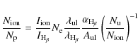
where
The results are given in Table 6, where the first column lists the ion
concerned, and the second column the line used for the abundance
determination. The third column gives the intensity of the line used
relative to
![]() .
The fourth column gives the temperature used
for the ion, the fifth column shows the ionic abundances, and the
sixth column gives the Ionization Correction Factor (ICF). This has
been determined empirically, usually by looking at the ionization potential
of the missing ion. Notice that the ICF is unity for all elements except for
Ar, S and Cl where it is close to unity. The exception to this is for Si and
Mg where only single
ionization stages are measured. In these two cases the ICF is
estimated with the help of the model described below. In the other
cases the element abundances, given in the last column, are probably
well determined. The abundance of carbon is more uncertain than the
other elements because both, the C III] and C IV lines, are quite
sensitive to the electron temperature.
.
The fourth column gives the temperature used
for the ion, the fifth column shows the ionic abundances, and the
sixth column gives the Ionization Correction Factor (ICF). This has
been determined empirically, usually by looking at the ionization potential
of the missing ion. Notice that the ICF is unity for all elements except for
Ar, S and Cl where it is close to unity. The exception to this is for Si and
Mg where only single
ionization stages are measured. In these two cases the ICF is
estimated with the help of the model described below. In the other
cases the element abundances, given in the last column, are probably
well determined. The abundance of carbon is more uncertain than the
other elements because both, the C III] and C IV lines, are quite
sensitive to the electron temperature.
Table 6: Ionic concentrations and chemical abundances in NGC 2792.
4 Model
In order to obtain as nearly a correct model as possible, the star as well as the nebula must be considered. Modeling the nebula-star complex will allow characterizing not only the central star's temperature but other stellar parameters as well (i.e., log g and luminosity). It can determine distance and other nebular properties, especially the composition, including the composition of elements that are represented by a single stage of ionization, which cannot be determined by the simplified analysis above. This method can take the presence of dust and molecules into account in the nebular material, when there is any there, making it a very comprehensive approach. While the line ratio method is simple and fast, the ICFs rest on uncertain physics. To this end, modeling serves as an effective means, and the whole set of parameters are determined in a unified way, assuring self consistency. Also, in this way one gets good physical insight into the PN, the method and the observations. Thus, modeling is a good approach to an end-to-end solution to the problem.
It is with this in mind that we have constructed a photoionization model for NGC 2792 with the code Cloudy, using the latest version C08.00 of Aug. 2008. (Ferland et al. 1998). Information on the updates in this version can be found on Cloudy's website.
4.1 Assumptions
Looking at the HST visual image shown in Fig. 1, it is reasonable to assume that the nebula is nearly spherical. We then determined its angular radius as 10 arcsec from this image. Initially we also assumed in the model that the spatial variation of density is minimal so a constant density model would be sufficient. But later, after some trial runs, we thought it appropriate to use a model in which the density varies radially across the nebula. The HST image being a broadband visual one, H-alpha images give a better estimate of the actual density (N(H)/cc). Therefore we used the H-alpha image of this PN from http://astro.uni-tuebingen.de/groups/pn/. This image was downloaded and used as is, since no additional information was available about it. We could import it into the IRAF facility and about 30 cross-cuts (i.e., density profiles) were taken over several clock positions and averaged. It should be noted that at this stage this average profile represents neither an emission measure nor true density. It is simply a count vs. pixel profile since the original image does not have any information on whether it is fully processed and intensity calibrated. This profile was then smoothed, used as a template, and converted to density vs angular radius using a radius of 10 arcsec for the nebula, since the template only gives counts vs pixels. The counts were then normalized to N(H)/cc assuming a nominal value of 3000/cc for the peak of the profile. Later in the actual modeling process, we not only allowed the distance to be a free parameter (affecting the radial profile since any change in distance changes the linear radius) but also varied the density by enhancing or decreasing the actual N(H)/cc value at each radial point. The profile used in the final model is shown in Fig. 3. Because determinating the density is difficult using line ratios, the above method was thought to be the best alternative. We have included dust grains mixed with gas in the nebula, so that we could compare model dust grain emission continua with the Spitzer observations. To represent the central star's ionizing radiation, we experimented with several model atmospheres available within the built-in library of Cloudy. We also tried pure black-body radiation in some test models.
4.2 Results
The general method of applying the code Cloudy to model NGC 2792 is the same as in Surendiranath et al. (2004). We ran a number of models and each time the output was carefully scrutinized before running the next model with changed input parameters. We tried to match the observed spectral fluxes of about 70 lines and we relied on physical intuition rather than any of the optimization techniques provided in Cloudy. The results are presented in Tables 7 and 8 and discussed in more detail in the following section, where we treat the abundances determined by the empirical (ICF) method as our final values for this PN.
Table 7: Parameters representing the final model.
5 Discussion
After a number of models were computed as discussed in the previous
section, it gradually became clear that it was very difficult to
reproduce the observed emission line fluxes, especially those of
He II, C III] in the UV and [O IV] in the IR
region. The observed absolute H![]() flux could be reproduced
well. See the final model output spectra in Table 8. This was the
best that could be done with the many models we tested. The
corresponding input parameters are listed in Table 7. In the final
model, we used the Rauch (2003) model atmosphere to represent
the central star's ionizing radiation. We recommend the abundances as
determined by the empirical line ratio method for this PN and discuss some
important implications of our modeling exercise below.
flux could be reproduced
well. See the final model output spectra in Table 8. This was the
best that could be done with the many models we tested. The
corresponding input parameters are listed in Table 7. In the final
model, we used the Rauch (2003) model atmosphere to represent
the central star's ionizing radiation. We recommend the abundances as
determined by the empirical line ratio method for this PN and discuss some
important implications of our modeling exercise below.
Table 8:
The emission line fluxes (
![]() ).
).
5.1 Possible causes for non-convergence of the model
The basic problem is that none of our models tested could reproduce
the apparently very high level of emitted flux in lines of certain
ions mentioned above. Because of this high level of excitation we tried
modeling with first a binary and then with a very high temperature star.
As a binary for the CSPN we inputted
the energies of two different model atmospheres together, but this
did not help. We then tried a black-body model atmosphere of
![]() K and this also could not reproduce the line of
He II and [O IV] among others. The diagnostic lines
did not agree well with observed values. Changing other parameters
also did not work. Our final model was the best
we could achieve. One possibility for non-convergence of the
model output spectrum with the observations could be that the slits used to
obtain the various spectra are different and the combining of these various
spectra introduces errors which differ with the different lines. While this
must play a small role, most of the observations cover a substantial part
of the nebula, and, as already discussed, are always normalized to the same
H
K and this also could not reproduce the line of
He II and [O IV] among others. The diagnostic lines
did not agree well with observed values. Changing other parameters
also did not work. Our final model was the best
we could achieve. One possibility for non-convergence of the
model output spectrum with the observations could be that the slits used to
obtain the various spectra are different and the combining of these various
spectra introduces errors which differ with the different lines. While this
must play a small role, most of the observations cover a substantial part
of the nebula, and, as already discussed, are always normalized to the same
H![]() .
The optical measurements are generally made with a long
slit which is about 5
.
The optical measurements are generally made with a long
slit which is about 5
![]() wide and thus integrate about half of the
nebular light. The infrared LH measurement covers an even larger region of
the nebula (judging from the hydrogen lines more than 90% of the nebula
is seen) but the infrared SH covers a smaller region. Finally the UV
measurements cover only about one half of the nebula because they are not
well centered. However because all measurements integrate along the
line-of-sight we doubt that this is the cause of the discrepancy. Other
explanations include the possibility that this PN
has a central star that emits an unusual or peculiar energy spectrum,
such that no currently available model atmosphere can represent it. While
this cannot be ruled out it seems to us unlikely that such a hot star would
deviate substantially from a blackbody.
An alternative possibility is that the model's assumed geometry
is wrong. We had assumed a spherical shell based on the
visual image. The PN could possibly have a different geometry and still
have a circular appearance because the axis of symmetry is in the
line-of-sight. But no models with axi-symmetric geometry have been studied
in the literature so the effect of a different geometry cannot be
ascertained. Only dynamical studies will shed more light on a possible
axi-symmetric geometry for the nebula.
wide and thus integrate about half of the
nebular light. The infrared LH measurement covers an even larger region of
the nebula (judging from the hydrogen lines more than 90% of the nebula
is seen) but the infrared SH covers a smaller region. Finally the UV
measurements cover only about one half of the nebula because they are not
well centered. However because all measurements integrate along the
line-of-sight we doubt that this is the cause of the discrepancy. Other
explanations include the possibility that this PN
has a central star that emits an unusual or peculiar energy spectrum,
such that no currently available model atmosphere can represent it. While
this cannot be ruled out it seems to us unlikely that such a hot star would
deviate substantially from a blackbody.
An alternative possibility is that the model's assumed geometry
is wrong. We had assumed a spherical shell based on the
visual image. The PN could possibly have a different geometry and still
have a circular appearance because the axis of symmetry is in the
line-of-sight. But no models with axi-symmetric geometry have been studied
in the literature so the effect of a different geometry cannot be
ascertained. Only dynamical studies will shed more light on a possible
axi-symmetric geometry for the nebula.
The UV line at
![]() Å, could be due to [Fe IV] but this assumption required a very high iron abundance and hence we doubt its identification with that ion. This is true with regard to the line ratio method as well. The final model's input and output are
shown in tables only for the purpose of illustration of the
difficulties faced. It reproduced both the absolute H
Å, could be due to [Fe IV] but this assumption required a very high iron abundance and hence we doubt its identification with that ion. This is true with regard to the line ratio method as well. The final model's input and output are
shown in tables only for the purpose of illustration of the
difficulties faced. It reproduced both the absolute H![]() flux
(Table 8) and the grain emitted continuum in the IR (not shown here)
very well.
flux
(Table 8) and the grain emitted continuum in the IR (not shown here)
very well.
6 Comparison with other abundance determinations
Table 9 shows a comparison of our abundances with the most important determinations in the past 20 years. The agreement is not very good, differences of a factor of three or more are common. The probable reasons for this are discussed in the following subsection. A comparison is also made with the solar abundance (Grevesse et al. 2007) and is given in the last column.
The helium abundance has been derived using the theoretical work of
Benjamin et al. (1999) and Porter et al. (2005).
For recombination of singly ionized helium, most weight is given to
the ![]() 5875 Å line, because the theoretical determination of
this line is the most reliable.
5875 Å line, because the theoretical determination of
this line is the most reliable.
6.1 Errors
It is difficult to determine the errors in the abundance
determination. The reason for this is the following. The error can
occur at several stages in the determination. An error can occur in
the intensity determination and this can be specified: it is
probably less than 30% and may be lower for the stronger lines. An
error may occur in correcting for the extinction, either because the
extinction is incorrect or the average reddening law is not
applicable. We have tried to minimize this possibility by making
use of known atomic constants to relate the various parts of the
spectrum. Thus the ratio of the infrared spectrum to the visible
spectrum is fixed by the ratio of infrared hydrogen lines to H![]() which
is essentially an atomic constant.
which
is essentially an atomic constant.
In Table 1 the measurements of three hydrogen lines are given as well as the
observed ratio of these lines to H![]() .
We may compare these observed
ratios with the theoretical ratios for an electron temperature of 15 000 K.
Because the 12.368
.
We may compare these observed
ratios with the theoretical ratios for an electron temperature of 15 000 K.
Because the 12.368 ![]() m line is used to derive the observed H
m line is used to derive the observed H![]() the
ratio automatically agrees. The 7.478
the
ratio automatically agrees. The 7.478 ![]() m line which measures the 6-5, 8-6
and 17-8 transitions is expected to have a ratio of 2.67 compared to the
14% higher observed value of 3.05. The 11.309
m line which measures the 6-5, 8-6
and 17-8 transitions is expected to have a ratio of 2.67 compared to the
14% higher observed value of 3.05. The 11.309 ![]() m line is expected to have
a value of 0.253 whereas the observed value is 0.33. While this is a
difference of 30% the line is among the weakest observed and thus the
highest expected error.
m line is expected to have
a value of 0.253 whereas the observed value is 0.33. While this is a
difference of 30% the line is among the weakest observed and thus the
highest expected error.
Table 9: Comparison of abundances in NGC 2792.
6.2 Reasons for the difference
The most important reason that the abundances we obtain differ from
the earlier results in the literature is our ability to recognize
that a gradient of the electron temperature exists in the nebula.
This is easiest to see in the case of oxygen. All the earlier
results give an electron temperature from the O III line
ratio in the visual spectrum. Values are found for the temperature
between 12 000 and 14 200 K. From the same lines we find a similar
value, between 14 000 K and 15 000 K (see Table 5). Consequently we
find a value of the
![]() abundance which is similar to the
earlier results. The difference in the total oxygen abundance occurs
because in the earlier work this same temperature is used to
determine the
abundance which is similar to the
earlier results. The difference in the total oxygen abundance occurs
because in the earlier work this same temperature is used to
determine the
![]() abundance from the UV line at
1400 Å which gives a very high abundance for this ion. We are able
to use the infrared
abundance from the UV line at
1400 Å which gives a very high abundance for this ion. We are able
to use the infrared
![]() line, which is almost temperature
insensitive, to determine the
line, which is almost temperature
insensitive, to determine the
![]() abundance and find that
it really has a much lower value. The high nitrogen and carbon
abundance found by Kingsburgh & Barlow (1994) has the same
origin: too low an electron temperature was used in conjunction with
the ultraviolet lines of N III, N IV, C III and
C IV, which are all very temperature-sensitive. This emphasizes the
importance of using the temperature insensitive infrared lines. Notice that
our results demonstrate that the carbon abundance is only about half of the
oxygen abundance, while the work of Kingsburgh & Barlow (1994)
find carbon to be 50% higher than oxygen.
abundance and find that
it really has a much lower value. The high nitrogen and carbon
abundance found by Kingsburgh & Barlow (1994) has the same
origin: too low an electron temperature was used in conjunction with
the ultraviolet lines of N III, N IV, C III and
C IV, which are all very temperature-sensitive. This emphasizes the
importance of using the temperature insensitive infrared lines. Notice that
our results demonstrate that the carbon abundance is only about half of the
oxygen abundance, while the work of Kingsburgh & Barlow (1994)
find carbon to be 50% higher than oxygen.
A further error may be introduced by the correction for unseen stages of ionization. This varies with the element, but is usually small because very many ionization stages are observed. When the model is included the error due to missing stages of ionization becomes quite small.
7 Stellar evolution
The modeling exercise provides some clues regarding the nature of the
stellar energy distribution and the stellar luminosity and effective
temperature (see Table 7). These values may be compared to more
conventional methods. The
![]() found from the Zanstra method by
Gathier & Pottasch (1988) gives a hydrogen Zanstra
temperature of 82 000 K and a HeII Zanstra temperature of 135 000 K,
using a magnitude V=17.04. The Energy Balance method using the line
intensities in the first three tables of this paper and the theory of
Preite-Martinez & Pottasch (1983) leads to a temperature of
about 100 000 K. It is rather difficult to deduce a precise value of
the temperature. Ignoring the hydrogen Zanstra temperature because the
nebula may be optically thin to ionizing radiation, a reasonable, though
uncertain, average value is
found from the Zanstra method by
Gathier & Pottasch (1988) gives a hydrogen Zanstra
temperature of 82 000 K and a HeII Zanstra temperature of 135 000 K,
using a magnitude V=17.04. The Energy Balance method using the line
intensities in the first three tables of this paper and the theory of
Preite-Martinez & Pottasch (1983) leads to a temperature of
about 100 000 K. It is rather difficult to deduce a precise value of
the temperature. Ignoring the hydrogen Zanstra temperature because the
nebula may be optically thin to ionizing radiation, a reasonable, though
uncertain, average value is
![]() K. Using this value of
temperature and the above stellar magnitude and distance, the stellar radius is
0.068 R
K. Using this value of
temperature and the above stellar magnitude and distance, the stellar radius is
0.068 R![]() .
Combined with the above temperature, the luminosity
of the star is
.
Combined with the above temperature, the luminosity
of the star is
![]() L
L![]() .
This is a factor of 2 higher than
the value used in the modeling and is listed in Table 7. These two
values have been determined independently of each other, and
considering the uncertainties in their determination they agree within
a factor of two.
.
This is a factor of 2 higher than
the value used in the modeling and is listed in Table 7. These two
values have been determined independently of each other, and
considering the uncertainties in their determination they agree within
a factor of two.
The abundances in NGC 2792 are similar to the solar abundance and to
other PNe which are thought to originate from low mass stars. The
abundances are almost identical to those of IC 2448 (Guiles et al. 2007), the only differences larger than a factor of two
are the lower carbon and higher sulfur abundances in NGC 2792. Other
PNe with similar abundances are NGC 6210, NGC 6369 and NGC 7662.
All these nebulae have a low helium abundance, similar to the Sun, as
well as nitrogen abundances whose low values indicate that very little
nitrogen has been formed in the course of evolution. This is in
agreement with theoretical calculations of the evolution of stars
whose initial mass is close to 1 M![]() ,
e.g. Karakas
(2003).
,
e.g. Karakas
(2003).
8 Conclusions
New IR spectra of NGC 2792 from the Spitzer Space Telescope have been presented and are analyzed in conjunction with other archival spectra in the UV and optical range. The abundances of He, C, N, O, S, Ar, Ne and Cl are found by the empirical method.
We have attempted a photoionization model for this nebula and found that the observed spectra could not be reproduced fully satisfactorily and hence recommend the abundances determined by the empirical method although the differences are small. Abundances of Si and Mg were found using the ionization levels found by the model. We have speculated on possible causes for the non-convergence of the model which could be either because the central star radiation is difficult to determine (i.e., non-representable by current model atmospheres) or because the geometry of the nebula complicated (i.e., it may be bipolar) and hence spherical symmetry is non-applicable. The central star's parameters became difficult to determine from the model because of this. Nevertheless the model is useful in two ways. First, when used together with the observed spectrum it provides insight into the electron temperature gradient in the nebula. Second, it makes it possible to correct for the missing ionization stages, especially in the cases of Mg and Si, and thus makes meaningful abundance determinations possible for these elements.
The abundances found have been compared with those previously determined for this nebula. We show that rather large differences exist and are due largely to neglect of being able to recognize electron temperature gradients in the nebula in previous work.
The central star is also discussed. The temperature and luminosity of
the star have been determined. Together with the nebular abundances we
show that this star evolved from an initial mass close to 1 M![]() .
.
Acknowledgements
We duly acknowledge the use of SIMBAD and ADS in this research work. We have used the IUE spectra archive at the STSCI and we wish to thank the archive unit for the same.
References
- Benjamin, R. A., Skillman, E. D., & Smits, D. P. 1999, ApJ, 514, 307 [NASA ADS] [CrossRef] (In the text)
- Bernard Salas, J., Pottasch, S. R., Beintema, D. A., & Wesselius, P. R. 2001, A&A, 367, 949 [NASA ADS] [CrossRef] [EDP Sciences] (In the text)
- Cahn, J. H., Kaler, J. B., & Stanghellini, L. 1992, A&AS, 94, 399 [NASA ADS] (In the text)
- Corradi, R. L. M., Schonberner, D., Steffen, M., et al. 2003, MNRAS, 340, 417 [NASA ADS] [CrossRef] (In the text)
- Condon, J. J., & Kaplan, D. L. 1998, ApJS 117, 361
- Davey, A. R., Storey, P. J., & Kisielius, R. 2000, A&AS, 142, 85 [NASA ADS] [CrossRef] [EDP Sciences]
- Ferland, G. J., Korista, K. T., Verner, D. A., et al. 1998, PASP, 110, 761 [NASA ADS] [CrossRef] (In the text)
- Fluks, M. A., Plez, B., de Winter, D., et al. 1994, A&AS, 105, 311 [NASA ADS] (In the text)
- de Freitas Pacheco, J. A., Maciel, W. J., & Costa, R. D. D. 1992, A&A, 261, 579 [NASA ADS] (In the text)
- Gathier, R., & Pottasch, S. R. 1988, A&A, 197, 266 [NASA ADS] (In the text)
- Gathier, R., Pottasch, S. R., & Pel, J. W. 1986, A&A, 157, 171 [NASA ADS] (In the text)
- Grevesse, N., Asplund, M., & Sauval, A. J. 2007, Sp. Sci. Rev., 130, 105 [NASA ADS] [CrossRef] (In the text)
- Gregory, P. C., Vavasour, J. D., Scott, W. K., et al. 1994, ApJS, 90, 173 [NASA ADS] [CrossRef] (In the text)
- Guiles, S., Bernard-Salas, J., Pottasch, S. R., et al. 2007, ApJ, 660, 1282 [NASA ADS] [CrossRef] (In the text)
- Henry, R. B. C., Kwitter, K. B., & Balick, B. 2005, AJ, 127, 2284 [NASA ADS] [CrossRef] (In the text)
- Higdon, S. J. U., Devost, D., Higdon, J. L., et al. 2004, PASP, 116, 975 [NASA ADS] [CrossRef] (In the text)
- Houck, J. R., Appleton, P. N., Armus, L., et al. 2004, ApJS, 154, 18 [NASA ADS] [CrossRef] (In the text)
- Hummer, D. G., & Storey, P. J. 1987, MNRAS, 224, 801 [NASA ADS] (In the text)
- Karakas, A. I. 2003, Thesis, Monash Univ. Melbourne (see also Karakas, A., & Lattanzio, J. C. 2007, PASA 24, 103) (In the text)
- Kerber, F., Mignani, R. P., Guglielmetti, F., & Wicenec, A. 2003, A&A, 408, 1029 [NASA ADS] [CrossRef] [EDP Sciences] (In the text)
- Kingsburgh, R. L., & Barlow, M. J. 1994, MNRAS, 271, 257 [NASA ADS] (In the text)
- Milingo, J. B., Kwitter, K. B., Henry, R. B. C., et al. 2002a, ApJS, 138, 279 [NASA ADS] [CrossRef] (In the text)
- Milingo, J. B., Henry, R. B. C., & Kwitter, K. B. 2002b, ApJS, 138, 285 [NASA ADS] [CrossRef]
- Porter, R. L., Bauman, R. P., Ferland, G. J., et al. 2005, ApJ, 622, L73 [NASA ADS] [CrossRef] (In the text)
- Pottasch, S. R., & Acker, A. 1989, A&A, 221, 123 [NASA ADS]
- Pottasch, S. R., & Beintema, D. A. 1999, A&A, 347, 974 (In the text)
- Pottasch, S. R., Wesselius, P. R., Wu, C. C., et al. 1977, A&A, 54, 435 [NASA ADS]
- Pottasch, S. R., Dennefeld, M., & Mo, J.-E. 1986a, A&A, 155, 397 [NASA ADS]
- Pottasch, S. R., Preite-Martinez, A., Olnon, F. M., et al. 1986b, A&A, 161, 363 [NASA ADS]
- Pottasch, S. R., Beintema, D. A., & Feibelman, W. A. 2000, A&A, 363, 767 [NASA ADS] (In the text)
- Pottasch, S. R., Beintema, D. A., Bernard Salas, J., & Feibelman, W. A. 2001, A&A, 380, 684 [NASA ADS] [CrossRef] [EDP Sciences] (In the text)
- Pottasch, S. R., Beintema, D. A., Bernard Salas, J., et al. 2002, A&A, 393, 285 [NASA ADS] [CrossRef] [EDP Sciences]
- Preite-Martinez, A., & Pottasch, S. R. 1983 A&A, 126, 31 (In the text)
- Rauch, T. 2003, A&A, 403, 709 [NASA ADS] [CrossRef] [EDP Sciences] (In the text)
- Surendiranath, R., Pottasch, S. R., & García-Lario, P. 2004, A&A, 421, 1051 [NASA ADS] [CrossRef] [EDP Sciences] (In the text)
- Torres-Peimbert, S., & Peimbert. M. 1977, RMxAA, 2, 181 [NASA ADS] (In the text)
- Wright, A. E., Griffith, M. R., Burke, B. F., & Ekers, R. D. 1994, ApJS, 91, 111 [NASA ADS] [CrossRef] (In the text)
Footnotes
- ... NGC 2792
- Based on observations with the Spitzer Space Telescope, which is operated by the Jet Propulsion Laboratory, California Institute of Technology.
All Tables
Table 1: IRS spectrum of NGC 2792.
Table 2: Visual spectrum of NGC 2792.
Table 3: IUE spectrum of NGC 2792.
Table 4: Electron density indicators in NGC 2792.
Table 5: Electron temperature indicators in NGC 2792.
Table 6: Ionic concentrations and chemical abundances in NGC 2792.
Table 7: Parameters representing the final model.
Table 8:
The emission line fluxes (
![]() ).
).
Table 9: Comparison of abundances in NGC 2792.
All Figures
| |
Figure 1: HST image of NGC 2792; Credits: Howard Bond; HST archived exposures catalog (STSCI, 2007). |
| Open with DEXTER | |
| In the text | |
| |
Figure 2:
The IRS spectrum of NGC/,2792. The SH intensity (from 9.9 |
| Open with DEXTER | |
| In the text | |
| |
Figure 3: The input density profile. The ordinate is the electron density. |
| Open with DEXTER | |
| In the text | |
Copyright ESO 2009
Current usage metrics show cumulative count of Article Views (full-text article views including HTML views, PDF and ePub downloads, according to the available data) and Abstracts Views on Vision4Press platform.
Data correspond to usage on the plateform after 2015. The current usage metrics is available 48-96 hours after online publication and is updated daily on week days.
Initial download of the metrics may take a while.