| Issue |
A&A
Volume 502, Number 1, July IV 2009
|
|
|---|---|---|
| Page(s) | 401 - 408 | |
| Section | Astronomical instrumentation | |
| DOI | https://doi.org/10.1051/0004-6361/200912006 | |
| Published online | 27 May 2009 | |
Robust correlators
P. Fridman
ASTRON, Oudehoogeveensedijk 4, Dwingeloo, 7991PD, The Netherlands
Received 8 March 2009 / Accepted 19 April 2009
Abstract
Context. Radio frequency interference (RFI) already limits the sensitivity of existing radio telescopes in several frequency bands and may prove to be an even greater obstacle for future generation instruments to overcome.
Aims. I aim to create a structure of radio astronomy correlators which will be statistically stable (robust) in the presence of interference.
Methods. A statistical analysis of the mixture of system noise + signal noise + RFI is proposed here which could be incorporated into the block diagram of a correlator. Order and rank statistics are especially useful when calculated in both temporal and frequency domains.
Results. Several new algorithms of robust correlators are proposed and investigated here. Computer simulations and processing of real data demonstrate the efficacy of the proposed algorithms.
Key words: instrumentation: interferometers - methods: data analysis - methods: statistical
1 Introduction
Correlators are central to the signal processing system of radio interferometer, (Thompson et al. 2001). Signals received from radio sources mixed with system noise (sky noise + receiver noise) can be represented as stochastic processes with a Gaussian (normal) distribution. Each pair of random numbers at the input of the correlator
is described as a bivariate random value (X,Y) with the distribution
![]() where
where
![]() are the mean values,
are the mean values,
![]() and
and
![]() are variances proportional to the intensity of the input noise and
are variances proportional to the intensity of the input noise and ![]() is the correlation coefficient (normalized visibility for a particular baseline). From the sequences
x1,...,xN and
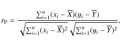
y1,...,yN the correlator calculates the so-called Pearson's correlation coefficient
is the correlation coefficient (normalized visibility for a particular baseline). From the sequences
x1,...,xN and
y1,...,yN the correlator calculates the so-called Pearson's correlation coefficient
 |
(1) |
where
The sample correlation coefficient ![]() is very sensitive to outliers (samples which are not consistent with the normal distribution
is very sensitive to outliers (samples which are not consistent with the normal distribution
![]() ,
.i.e., the estimate (1) is not statistically robust (Gnanadesikan 1997; Huber 1981).
Radio frequency interference (RFI) can produce considerable outliers, yielding a bias of
,
.i.e., the estimate (1) is not statistically robust (Gnanadesikan 1997; Huber 1981).
Radio frequency interference (RFI) can produce considerable outliers, yielding a bias of ![]() and increasing the standard deviation (rms) of
and increasing the standard deviation (rms) of ![]() .
In this paper the terms ``RFI'' and ``outliers'' are interchangeable.
.
In this paper the terms ``RFI'' and ``outliers'' are interchangeable.
Methods of robust statistics allow stable estimates to be obtained in the presence of outliers in several radio-astronomical applications (Fridman 2008). Here these methods are applied to correlation measurements of radio interferometers.
There are different types of RFI (Fridman & Baan 2001) and they differ significantly over the radio astronomy frequency band. Strong and impulse-like RFI on the time-frequency plane are visible in practically all frequency bands of LOFAR, and these types of RFI are considered here because data from the LOFAR Core Station (CS1) are used as examples later in this paper. Figure 1 gives an impression of the types of interferences in one sub-band: the auto-spectrum of the system noise + RFI from the LOFAR CS1 is represented in this figure with high spectral and time resolution.
![\begin{figure}
\par\includegraphics[width=8cm,clip]{12006fg1.eps}
\end{figure}](/articles/aa/full_html/2009/28/aa12006-09/img37.png) |
Figure 1:
Autospectrum of system noise + RFI from LOFAR CS1 at the central frequency
f0=217.1875 MHz, bandwidth
|
| Open with DEXTER | |
The following approximate classification is proposed for the strong RFI visible at LOFAR:
- a)
- narrow-band and persistent RFI;
- b)
- narrow impulses (<1 s, <100 Hz) on the time-frequency plane;
- c)
- impulse-like RFI in the time domain (several seconds) which are also wide-band (5-10 MHz);
- d)
- random-form bursts on the time-frequency plane.
Several types of robust correlators that are able to mitigate the impulse-like, strong RFI in both temporal and frequency domains have been studied in this paper. They are used in applications where input data are contaminated with outliers, and these correlators are statistically more stable than correlator (1). Some of them could be used in radio astronomy, especially in radio interferometric systems with software correlators where the calculation of visibilities is carried out on general-purpose computers, as in LOFAR (2009) and JIVE (Kruithof2009). Software correlators are, by definition, much more flexible than traditional hardware correlators: any algorithm adapted or modified for a particular observation can be optionally downloaded as a subroutine.
There are two operations in the numerator of (1): multiplication of the input samples of X and Y and summation (averaging). Here it is proposed that they be modified to make the correlator more robust.
The new features can be introduced in the first operation to analyze the statistics of X and Y and to introduce a type of editing in order to eliminate outliers.
The second operation, summation, which is considered as post-correlation averaging, can be divided into three steps: primary averaging over a time interval which is not too long to smooth RFI bursts appearing at this stage above the noise level, RFI mitigation and secondary averaging to the required time interval depending on the observational specifications (wavelength, baseline, radio source properties), see end of Sect. 3 and Figs. 13-15.
Different types of correlators described in the following section are compared with Pearson's correlator (1) using two criteria:
- 1.
- the bias of the estimate
 produced by RFI compared to the input correlation coefficient
  ;
;
- 2.
- the effectiveness of an estimator is judged by the rms at the output of the correlator in both the presence and in the absence of outliers.
2 Estimators of the correlation coefficient
There are two classic estimators of correlation coefficients using ranks of samples instead of the samples themselves, (Kendall 1970).
Let two input sample sequences
x1,...xn and
y1,...yn be sorted in ascending order:
![]() and
and
![]() .
The ith value x(i) is called ith-order statistic. Each sample xj has its kth position in the sorted series
x(1),...x(n). This number k is the rank of the sample xj and is denoted by pj(=k). Similarly, the rank of yj is denoted by qj. Let
(xi,yi) and
(xj,yj) with i=1,...n and
j=i+1,...n be two data pairs from the original data sequences. If
pj-pi and
qj-qi have the same sign, these two data pairs are said to be concordant, otherwise, they are discordant. Let
.
The ith value x(i) is called ith-order statistic. Each sample xj has its kth position in the sorted series
x(1),...x(n). This number k is the rank of the sample xj and is denoted by pj(=k). Similarly, the rank of yj is denoted by qj. Let
(xi,yi) and
(xj,yj) with i=1,...n and
j=i+1,...n be two data pairs from the original data sequences. If
pj-pi and
qj-qi have the same sign, these two data pairs are said to be concordant, otherwise, they are discordant. Let ![]() be the number of concordant pairs and
be the number of concordant pairs and ![]() the number of discordant pairs. It is clear that
the number of discordant pairs. It is clear that
![]() .
.
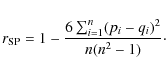
2.1 Spearman's correlator
The Spearman's correlation coefficient is calculated by
 |
(2) |
The bivariate correlation coefficient corresponding to Pearson's
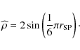 |
(3) |
2.2 Kendall's correlator
Kendall's correlation coefficient is calculated by
 |
(4) |
The bivariate correlation coefficient corresponding to Pearson's
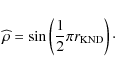 |
(5) |
2.3 Correlator using sums and differences
One of the first constructions of a robust correlator is based on the quarter square identity (Gnanadesikan & Kettenring 1972; Huber 1981):
| (6) |
where cov denotes covariance and var denotes variance. The correlation coefficient can be obtained with
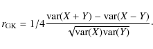 |
(7) |
Therefore, any robust estimators of variance can be used for this correlator (Fridman 2008). Several of them are applied here to (7).
2.3.1 Trimming
Samples
Z1 = X + Y and
Z2 = X - Y are sorted in ascending order:
z(1),...z(n). Let ![]() denote the chosen amount of trimming,
denote the chosen amount of trimming,
![]() and
and
![]() .
Sample-trimmed variance is computed by removing k of the largest and k of the smallest data and using the values that remain:
.
Sample-trimmed variance is computed by removing k of the largest and k of the smallest data and using the values that remain:
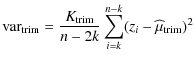 |
(8) | ||
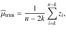 |
where
2.3.2 Winsorization
A sample Z is sorted in ascending order. For the chosen
![]() and
and
![]() ,
Winsorization
of the sorted data consists of setting
,
Winsorization
of the sorted data consists of setting
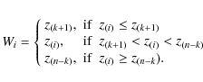 |
(9) |
The Winsorized sample mean is
 |
(10) |
The essence of Winsorization is to replace the k of the lowest and k of the highest samples of the sorted data z by the values of their nearest neighbors z(k+1) and z(n-k), respectively.
2.3.3 Median absolute deviation (MAD)
This estimate of the variance of sorted data
![]() is defined by
is defined by
 |
(11) |
where
Using
2.3.4 Qn estimate
This estimate is proposed in Rousseuw & Croux (1993)
and is moderately effective. It combines the ideas of the Hodges-Lehmann estimate and the Gini estimate, (Kendal & Stuart 1967):
 |
(12) |
where
Other robust algorithms can also be applied for example, the M-estimator, (Huber 1981) but here I was not attempting to make a comprehensive study of all types of robust correlators. Rather I wished to direct attention to the options hitherto unused in designing correlators.
3 Testing the algorithms
3.1 Mitigation of outliers in the temporal domain
The two input signals X and Y are modeled by bivariate random numbers with normal distribution, zero mean, standard deviation
![]() and correlation coefficient
and correlation coefficient
![]() .
Such
.
Such ![]() are typical of many radio interferometric observations when weak signals are processed. The number of samples in each data sequence is n and the number of repetitions of the correlation is m.
Outliers rfii added to the inputs xi and yi are modeled by the following expression:
are typical of many radio interferometric observations when weak signals are processed. The number of samples in each data sequence is n and the number of repetitions of the correlation is m.
Outliers rfii added to the inputs xi and yi are modeled by the following expression:
| (13) |
where si is the Poisson random value with the parameter
![\begin{figure}
\par\includegraphics[width=8cm,clip]{12006fg2.eps}
\end{figure}](/articles/aa/full_html/2009/28/aa12006-09/img80.png) |
Figure 2: Input signals representing Gaussian noise + impulse-like outliers, the number of samples n=10 000. |
| Open with DEXTER | |
Table 1:
Bias and rms of
![]() for the Spearman and Kendall correlators,
n=1000, m=1000, 95%-confidence intervals for bias:
for the Spearman and Kendall correlators,
n=1000, m=1000, 95%-confidence intervals for bias:
![]() ,
for rms:
,
for rms:
![]() .
.
Table 2:
Bias and rms of
![]() for trimming,
for trimming,
![]() ,
95%-confidence intervals
for bias:
,
95%-confidence intervals
for bias:
![]() ,
for rms:
,
for rms:
![]() .
.
Table 3:
Bias and rms of
![]() for Winsorization,
for Winsorization,
![]() ,
,
![]() -confidence intervals for bias:
-confidence intervals for bias:
![]() ,
for rms:
,
for rms:
![]() .
.
Table 4:
Bias and rms of
![]() for median absolute deviation (MAD),
n = 1000, m = 10 000, 95%-confidence intervals for bias:
for median absolute deviation (MAD),
n = 1000, m = 10 000, 95%-confidence intervals for bias:
![]() ,
for rms:
,
for rms:
![]() .
.
Table 5:
Bias and rms of
![]() for Q2-estimator, n = 1000, m = 1000, 95%-confidence intervals
for bias:
for Q2-estimator, n = 1000, m = 1000, 95%-confidence intervals
for bias:
![]() ,
for rms:
,
for rms:
![]() .
.
The results of computer simulations, bias and rms of the estimate of
![]() are presented in Tables 1-5. The bias of the estimate
are presented in Tables 1-5. The bias of the estimate
![]() is:
is:
![]() .
The confidence intervals are calculated for the 95%-confidence level
and for
.
The confidence intervals are calculated for the 95%-confidence level
and for
![]() for
for
![]() and
and
![]() for rms (the approximations that are valid for small
for rms (the approximations that are valid for small ![]() and large mn).
and large mn).
Looking at Tables 1-5 several remarks can be made:
- 1.
- in the absence of outliers, robust correlators reproduce practically the same values of
as the Pearson's correlator (not showing a significant bias) and keeping the effectiveness close to
 (except MAD). Figure 3 shows this for correlator (7) with Winsorization;
- 2.
- the output of the Pearson's correlator is dramaticaly decorrelated with the growth of the outlier's amplitudes whereas robust correlators analyze local statistics (n samples) and eliminate outliers regardless of their amplitudes, see Fig. 4;
- 3.
- in the presence of outliers, robust correlators show a small positive bias which is equal to

 of
of  ;
;
- 4.
- Spearman's and Kendall's correlators (Table 1) provide a considerable reduction of bias in the presence of RFI compared to the reduction of bias in Pearson's correlator and keep the rms, i.e., there is no loss in effectiveness within the limits of error. These correlators require more operating capacity per lag, due to the sorting and ranking of samples (this is also valid for the following algorithms);
- 5.
- trimming and Winsorization (Tables 2 and 3) show good results with regard to bias and effectiveness. The rms for trimming is increased 10% than for Winsorization. The choice of
 presumes a percentage of outliers of less than 10%. So there is a considerable safety margin here but the growth of rms for
is insignificant. In practice, an adaptive choice of
presumes a percentage of outliers of less than 10%. So there is a considerable safety margin here but the growth of rms for
is insignificant. In practice, an adaptive choice of  is possible in each sub-band when the value of
is chosen after taking into account a real RFI environment situation, i.e., the presence or absence of RFI and its duty cycle;
is possible in each sub-band when the value of
is chosen after taking into account a real RFI environment situation, i.e., the presence or absence of RFI and its duty cycle;
- 6.
- median absolute deviation (MAD) (Table 4) gives the best results for the bias, but as predicted theoretically, it has the largest rms: 1.65 greater than
;
- 7.
- the Qn estimate (Table 5) requires more operating capacity than the others. The bias is as little as for the other algorithms, the rms is slightly larger (10%) than
;
- 8.
- the proposed methods are effective in the presence of strong impulse-like outliers. When not intercepted, they decorrelate the correlator's output and it is practically impossible to improve this situation with subsequent processing. Low-amplitude outliers are more difficult to detect because they are similar to the rare Gaussian noise spikes, but their decorrelation impact is also much weaker. For example, with an RFI amplitude
 ,
,
 and
and
 (signal-of-interest), the output of Pearson's correlator
is 0.092 and the output of Spearman's correlator 0.098;
(signal-of-interest), the output of Pearson's correlator
is 0.092 and the output of Spearman's correlator 0.098;
- 9.
- the situation is different when outliers are correlated at the inputs of the correlator. In this case outliers produce an excessive, false correlation even
in the absence of a signal-of-interest,
 .
For example, for strong 100%-correlated RFI with an amplitude equal to 30.0
.
For example, for strong 100%-correlated RFI with an amplitude equal to 30.0 ,
,
 and
,
the output of Pearson's correlator
is 0.349 and the output of the MAD-correlator is 0.001.
and
,
the output of Pearson's correlator
is 0.349 and the output of the MAD-correlator is 0.001.
For correlated RFI, other methods exploiting this correlation property can be more effective, see (Ellingson & Hampson 2003; Jeff et al. 2005; Kesteven 2007; Cornwell et al. 2004).
![\begin{figure}
\par\includegraphics[width=8cm,clip]{12006fg3.eps}
\end{figure}](/articles/aa/full_html/2009/28/aa12006-09/img92.png) |
Figure 3:
Correlation coefficients in the absence of outliers for Pearson's correlator (1), ( upper panel), and Winsorized correlator (7), ( lower panel), each of the m=100 correlation coefficients are calculated for n=1000 data samples, |
| Open with DEXTER | |
![\begin{figure}
\par\includegraphics[width=8cm,clip]{12006fg4.eps}
\end{figure}](/articles/aa/full_html/2009/28/aa12006-09/img93.png) |
Figure 4:
Correlation coefficients in the presence of outliers for Pearson's correlator (1), ( upper panel), and Winsorized correlator (7), ( lower panel),
|
| Open with DEXTER | |
3.2 Mitigation of outliers in the frequency domain
Narrow-band RFI can be detected as an impulse-like outlier in the frequency domain. The following example illustrates the application of trimming (8) in this case. RFI is generated as a phase-modulated sinusoidal carrier, see Fig. 5. The power spectrum of the unmodulated carrier is shown in the upper panel and in the lower panel, the power spectrum of the randomly phase-modulated signal is represented:
| (14) |
where rect(i) is a rectangular wave with Poisson's law distributed random jumps from -1 to +1, and the parameter of Poisson distribution
![\begin{figure}
\par\includegraphics[width=8cm,clip]{12006fg5.eps}
\end{figure}](/articles/aa/full_html/2009/28/aa12006-09/img95.png) |
Figure 5:
Power spectra of the unmodulated sinusoidal carrier ( upper panel) and the randomly-phased modulated carrier with the phase jumps |
| Open with DEXTER | |
![\begin{figure}
\par\includegraphics[width=8cm,clip]{12006fg6.eps}
\end{figure}](/articles/aa/full_html/2009/28/aa12006-09/img97.png) |
Figure 6: Input signal x noise +RFI ( upper panel) and its power spectra ( upper middle panel), input signal y ( lower middle panel) and its power spectra ( lower panel). |
| Open with DEXTER | |
![\begin{figure}
\par\includegraphics[width=8cm,clip]{12006fg7.eps}
\end{figure}](/articles/aa/full_html/2009/28/aa12006-09/img98.png) |
Figure 7:
Pearson's correlator output ( upper panel) and the ``sum-difference'' correlator ouput ( lower panel), |
| Open with DEXTER | |
The statistics of the power spectra are analyzed following (8) and the indexes of outliers exceeding the level equal to the 1.5%-percentile are used to reject the samples of the complex spectra of signals
![]() and
and
![]() ,
where
,
where
![]() denotes the Fourier transform. These indexes are tagged with the indicator function ind(i) taking the numbers 0 or 1, i = 1...n and assigned to the sequence of n samples of the complex spectra
denotes the Fourier transform. These indexes are tagged with the indicator function ind(i) taking the numbers 0 or 1, i = 1...n and assigned to the sequence of n samples of the complex spectra
![]() and
and
![]() .
The ``sum-difference'' correlator (7) is used in the spectral domain (FX-correlator):
.
The ``sum-difference'' correlator (7) is used in the spectral domain (FX-correlator):
| (15) |
Robust variance using the trimming algorithm (8) is applied while calculating (15): outliers are marked by the indicator function
![\begin{figure}
\par\includegraphics[width=8cm,clip]{12006fg8.eps}
\end{figure}](/articles/aa/full_html/2009/28/aa12006-09/img106.png) |
Figure 8:
Pearson's correlator output ( upper panel) and the ``sum-difference'' correlator ouput ( lower panel),
|
| Open with DEXTER | |
![\begin{figure}
\par\includegraphics[width=8cm,clip]{12006fg9.eps}
\end{figure}](/articles/aa/full_html/2009/28/aa12006-09/img107.png) |
Figure 9:
Pearson's correlator output ( upper panel) and the ``sum-difference'' correlator ouput ( lower panel),
|
| Open with DEXTER | |
Of course, other post-correlation methods can be used in the case of narrow-band persistent RFI with a stable spatial orientation,
for example, (Cornwell et al. 2004). But in the case of
sporadic burst-like RFI, the proposed pre-correlation statistical analysis is more appropriate: only
![]() samples were used for each correlator input, which corresponds to a microsecond time scale for typical bandwidths.
samples were used for each correlator input, which corresponds to a microsecond time scale for typical bandwidths.
3.2.1 Processing of observational data
Several examples of applications of the aforementioned algorithms are presented here.
The auto-spectrum in Fig. 10 is calculated using the ``raw'' data recorded at LOFAR CS1 for three hours. Data consisting of complex eight-bit numbers and having a sample time interval equal to 6.4 ![]() s were recorded on the subband with central frequency
f0 = 205.781 MHz, bandwidth
s were recorded on the subband with central frequency
f0 = 205.781 MHz, bandwidth
![]() KHz. This time-frequency presentation corresponds to 32 frequency channels, i.e.,
the frequency resolution is
KHz. This time-frequency presentation corresponds to 32 frequency channels, i.e.,
the frequency resolution is
![]() KHz, and the integration time
KHz, and the integration time
![]() s.
s.
Figure 11 demonstrates the auto-spectrum calculated from the same data for 1024 frequency channels. The high spectral resolution,
![]() Hz, permits the separation of RFI spikes, i.e., not smoothing them, as would have been in the case of 32 channels, see Fig. 10. Only half of the 3-h duration auto-spectrum is shown in Fig. 11 (due to the constraints of computer memory). The auto-spectrum in Fig. 11 is calculated without any censoring of outliers.
Hz, permits the separation of RFI spikes, i.e., not smoothing them, as would have been in the case of 32 channels, see Fig. 10. Only half of the 3-h duration auto-spectrum is shown in Fig. 11 (due to the constraints of computer memory). The auto-spectrum in Fig. 11 is calculated without any censoring of outliers.
Figure 12 shows the ``cleaned'' auto-spectrum where Winsorization was applied. The Winsorized spectrum in Fig. 12 is smoothed so as to get a final frequency resolution
![]() KHz as in Fig. 10.
KHz as in Fig. 10.
![\begin{figure}
\par\includegraphics[width=7.5cm,clip]{12006f10.eps}
\end{figure}](/articles/aa/full_html/2009/28/aa12006-09/img110.png) |
Figure 10:
Auto-spectrum of system noise +RFI from LOFAR CS1 at the central frequency
f0 = 205.781 MHz, bandwidth
|
| Open with DEXTER | |
![\begin{figure}
\par\includegraphics[width=7.5cm,clip]{12006f11.eps}
\end{figure}](/articles/aa/full_html/2009/28/aa12006-09/img111.png) |
Figure 11:
Auto-spectrum of system noise +RFI from LOFAR CS1 at the central frequency
f0=205.781 MHz, bandwidth
|
| Open with DEXTER | |
![\begin{figure}
\par\includegraphics[width=7.5cm,clip]{12006f12.eps}
\end{figure}](/articles/aa/full_html/2009/28/aa12006-09/img112.png) |
Figure 12: Auto-spectrum of the same data as in Fig. 11 calculated with Winsorization. |
| Open with DEXTER | |
![\begin{figure}
\par\includegraphics[width=7.5cm,clip]{12006f13.eps}
\end{figure}](/articles/aa/full_html/2009/28/aa12006-09/img113.png) |
Figure 13:
Post-correlation cross-spectrum, central frequency
f0 = 131.4453 MHz, bandwidth
|
| Open with DEXTER | |
![\begin{figure}
\par\includegraphics[width=7.5cm,clip]{12006f14.eps}
\end{figure}](/articles/aa/full_html/2009/28/aa12006-09/img114.png) |
Figure 14: Post-correlation cross-spectrum from Fig. 13 with outliers removed. |
| Open with DEXTER | |
![\begin{figure}
\par\includegraphics[width=7.5cm,clip]{12006f15.eps}
\end{figure}](/articles/aa/full_html/2009/28/aa12006-09/img115.png) |
Figure 15: Averaged cross-spectra corresponding to Fig. 13 ( upper and middle (zoomed) panels) and to Fig. 14 ( lower panel). |
| Open with DEXTER | |
This example shows the importance of a sufficiently high frequency resolution. All RFI visible in Fig. 11 are invisible in the temporal domain; they are too weak and they are ``below'' the system noise. The low level of RFI also made it necessary to average the instantaneous power spectra obtained after each FFT. The number of averaged spectra is 256 and thus the time resolution in the Fig. 11 is
![]() s. The ripple structure clearly visible in the auto-spectra is produced by the transfer functions of LOFAR digital filters separating the whole input bandwidth into dozens of sub-bands with the partial bandwidths
s. The ripple structure clearly visible in the auto-spectra is produced by the transfer functions of LOFAR digital filters separating the whole input bandwidth into dozens of sub-bands with the partial bandwidths
![]() KHz (or 200 KHz).
KHz (or 200 KHz).
The censoring of outliers may also be useful in the case of post-correlation data produced by the LOFAR correlator. The filter bank of the LOFAR backend divides each of the 156 KHz-bandwidth sub-bands into 256 narrow ``sub-sub-bands'' with a bandwidth equal to 610.3516 Hz. The sample time interval after preliminary averaging is 1 s. This good time-frequency resolution allows the fine-grain structure of RFI to be seen.
The following example in Fig. 13 shows the post-correlation cross-spectrum on frequency f0 = 131.4453 MHz.
Figure 14 shows the corresponding Winsorized cross-spectrum and Fig. 15 shows the averaged cross-spectra along the whole time interval
![]() s - without Winsorization (upper and middle panels) and with Winsorization (lower panel). The weak correlated component (the signal-of-interest) is produced by some cross-polarization effects and bears a ripple structure similar to the auto-spectra.
s - without Winsorization (upper and middle panels) and with Winsorization (lower panel). The weak correlated component (the signal-of-interest) is produced by some cross-polarization effects and bears a ripple structure similar to the auto-spectra.
4 Conclusions
- 1.
- Estimates of the correlation coefficient are an important part of both classical and of robust statistics. Statistical analysis of raw data with the finest available time and frequency resolution can help during observations in an RFI contaminated environment. Growing concern about RFI pollution should persuade the radio astronomy community to pay more attention to the variety of algorithms developed in the realm of robust statistics. This framework of robust estimates puts the successfully tested blanking of RFI on a more stable foundation.
- 2.
- Statistically faithful, robust estimates of the correlation coefficient are especially appropriate for application in an impulse-like strong RFI environment. RFI is effectively suppressed and the accompanying bias and effectiveness are tolerable. The aforementioned robust algorithms can be usefully applied in these particular situations.
- 3.
- The choice of a particular algorithm depends upon the type and intensity of the RFI. The proportion of RFI presence in data is also important. The type of implementation may determine the choice: off-line or real-time. It is difficult to equip existing conventional hardware correlators with these tools. Future generations of radio telescopes (LOFAR, ATA, SKA) will generate such huge amounts of data that real-time processing is vital: DSP, FPGA or supercomputers are possible solutions. Software correlators are especially suited to the implementation of robust schemes as optional subroutines.
Acknowledgements
My discussions with Ger de Bruyn and Jan Noordam have been very helpful and I am grateful for their continued support.
References
- Cornwell, T. J., Perley, R. A., Golap, K., & Bhatnagar, S. 2004, EVLA Memo 86 (In the text)
- Devlin, S. J., Gnanadesikan, R., & Kettenring, J. R. 1975, Biometrica, 62, 531 [CrossRef]
- Ellingson, S. W., & Hampson, G. A. 2003, ApJS, 147, 167 [NASA ADS] [CrossRef] (In the text)
- Fridman, P. A. 2008 AJ, 135, 1810 (In the text)
- Fridman, P. A., & Baan, W. 2001, A&A, 378, 327 [NASA ADS] [CrossRef] [EDP Sciences] (In the text)
- Gnanadesikan, R., & Kettenring, J. R. 1972, Biometrics, 28, 81 [CrossRef] (In the text)
- Gnanadesikan, R. 1997, Methods for Statistical Data Analysis of Multivariate Observations (John Wiley & Sons, Inc.), Chap. 5.2.3 (In the text)
- Jeff, B. D., Li, L., & Warnick, K. 2005, IEEE Trans. Signal Process., 53, 439 [NASA ADS] [CrossRef] (In the text)
- Huber, P. J. 1981, Robust Statistics (John Wiley & Sons, Inc.), Chap. 8 (In the text)
- Kendall, M. G. 1970, Rank Correlation Methods, 4th edn (London: Griffin) (In the text)
- Kendall, M. G., & Stuart, A. 1967, The advanced theory of statistics (London: Griffin), 1, Chap. 3 (In the text)
- Kesteven, M. 2007, URSI Radio Sci. Bull., 322, 9 (In the text)
- Kruithof, N. 2009, Signals and Communication Technology (US: Springer), 537 (In the text)
- LOFAR, http://www.lofar.org/p/systems_centrprocess.htm (In the text)
- Rousseuw, P. J., & Croux, C. 1993, J. Amer. Stat. Assoc., 88, 1273 [CrossRef]
- Thompson, A. R., Moran, J. M., & Swenson, G. W. 2001, Interferometry and Synthesis in Radio Astronomy (John Wiley & Sons, Inc.), Chap. 8 (In the text)
All Tables
Table 1:
Bias and rms of
![]() for the Spearman and Kendall correlators,
n=1000, m=1000, 95%-confidence intervals for bias:
for the Spearman and Kendall correlators,
n=1000, m=1000, 95%-confidence intervals for bias:
![]() ,
for rms:
,
for rms:
![]() .
.
Table 2:
Bias and rms of
![]() for trimming,
for trimming,
![]() ,
95%-confidence intervals
for bias:
,
95%-confidence intervals
for bias:
![]() ,
for rms:
,
for rms:
![]() .
.
Table 3:
Bias and rms of
![]() for Winsorization,
for Winsorization,
![]() ,
,
![]() -confidence intervals for bias:
-confidence intervals for bias:
![]() ,
for rms:
,
for rms:
![]() .
.
Table 4:
Bias and rms of
![]() for median absolute deviation (MAD),
n = 1000, m = 10 000, 95%-confidence intervals for bias:
for median absolute deviation (MAD),
n = 1000, m = 10 000, 95%-confidence intervals for bias:
![]() ,
for rms:
,
for rms:
![]() .
.
Table 5:
Bias and rms of
![]() for Q2-estimator, n = 1000, m = 1000, 95%-confidence intervals
for bias:
for Q2-estimator, n = 1000, m = 1000, 95%-confidence intervals
for bias:
![]() ,
for rms:
,
for rms:
![]() .
.
All Figures
| |
Figure 1:
Autospectrum of system noise + RFI from LOFAR CS1 at the central frequency
f0=217.1875 MHz, bandwidth
|
| Open with DEXTER | |
| In the text | |
| |
Figure 2: Input signals representing Gaussian noise + impulse-like outliers, the number of samples n=10 000. |
| Open with DEXTER | |
| In the text | |
| |
Figure 3:
Correlation coefficients in the absence of outliers for Pearson's correlator (1), ( upper panel), and Winsorized correlator (7), ( lower panel), each of the m=100 correlation coefficients are calculated for n=1000 data samples, |
| Open with DEXTER | |
| In the text | |
| |
Figure 4:
Correlation coefficients in the presence of outliers for Pearson's correlator (1), ( upper panel), and Winsorized correlator (7), ( lower panel),
|
| Open with DEXTER | |
| In the text | |
| |
Figure 5:
Power spectra of the unmodulated sinusoidal carrier ( upper panel) and the randomly-phased modulated carrier with the phase jumps |
| Open with DEXTER | |
| In the text | |
| |
Figure 6: Input signal x noise +RFI ( upper panel) and its power spectra ( upper middle panel), input signal y ( lower middle panel) and its power spectra ( lower panel). |
| Open with DEXTER | |
| In the text | |
| |
Figure 7:
Pearson's correlator output ( upper panel) and the ``sum-difference'' correlator ouput ( lower panel), |
| Open with DEXTER | |
| In the text | |
| |
Figure 8:
Pearson's correlator output ( upper panel) and the ``sum-difference'' correlator ouput ( lower panel),
|
| Open with DEXTER | |
| In the text | |
| |
Figure 9:
Pearson's correlator output ( upper panel) and the ``sum-difference'' correlator ouput ( lower panel),
|
| Open with DEXTER | |
| In the text | |
| |
Figure 10:
Auto-spectrum of system noise +RFI from LOFAR CS1 at the central frequency
f0 = 205.781 MHz, bandwidth
|
| Open with DEXTER | |
| In the text | |
| |
Figure 11:
Auto-spectrum of system noise +RFI from LOFAR CS1 at the central frequency
f0=205.781 MHz, bandwidth
|
| Open with DEXTER | |
| In the text | |
| |
Figure 12: Auto-spectrum of the same data as in Fig. 11 calculated with Winsorization. |
| Open with DEXTER | |
| In the text | |
| |
Figure 13:
Post-correlation cross-spectrum, central frequency
f0 = 131.4453 MHz, bandwidth
|
| Open with DEXTER | |
| In the text | |
| |
Figure 14: Post-correlation cross-spectrum from Fig. 13 with outliers removed. |
| Open with DEXTER | |
| In the text | |
| |
Figure 15: Averaged cross-spectra corresponding to Fig. 13 ( upper and middle (zoomed) panels) and to Fig. 14 ( lower panel). |
| Open with DEXTER | |
| In the text | |
Copyright ESO 2009
Current usage metrics show cumulative count of Article Views (full-text article views including HTML views, PDF and ePub downloads, according to the available data) and Abstracts Views on Vision4Press platform.
Data correspond to usage on the plateform after 2015. The current usage metrics is available 48-96 hours after online publication and is updated daily on week days.
Initial download of the metrics may take a while.