| Issue |
A&A
Volume 502, Number 1, July IV 2009
|
|
|---|---|---|
| Page(s) | 27 - 35 | |
| Section | Cosmology (including clusters of galaxies) | |
| DOI | https://doi.org/10.1051/0004-6361/200911881 | |
| Published online | 19 May 2009 | |
The residual gravity acceleration effect in the Poincaré dodecahedral space
B. F. Roukema - P. T. Rózanski
Torun Centre for Astronomy, Nicolaus Copernicus University, ul. Gagarina 11, 87-100 Torun, Poland
Received 19 February 2009 / Accepted 17 March 2009
Abstract
Context. In a flat space, it has been shown heuristically that the global topology of comoving space can affect the dynamics expected in the weak-field Newtonian limit, inducing a weak acceleration effect similar to dark energy.
Aims. Does a similar effect occur in the case of the Poincaré dodecahedral space, which is a candidate model of comoving space for solving the missing fluctuations problem observed in cosmic microwave background all-sky maps? Moreover, does the effect distinguish the Poincaré space from other well-proportioned spaces?
Methods. The acceleration effect in the Poincaré space S3/I* is studied, using a massive particle and a nearby test particle of negligible mass. Calculations are made in S3 embedded in
![]() .
The weak-limit gravitational attraction on a test particle at distance r is set to be
.
The weak-limit gravitational attraction on a test particle at distance r is set to be
![]() rather than
rather than
![]() ,
where
,
where
![]() is the curvature radius, in order to satisfy Stokes' theorem. A finite particle horizon large enough to include the adjacent topological images of the massive particle is assumed. The regular, flat, 3-torus T3 is re-examined, and two other well-proportioned spaces, the octahedral space S3/T*, and the truncated cube space S3/O*, are also studied.
is the curvature radius, in order to satisfy Stokes' theorem. A finite particle horizon large enough to include the adjacent topological images of the massive particle is assumed. The regular, flat, 3-torus T3 is re-examined, and two other well-proportioned spaces, the octahedral space S3/T*, and the truncated cube space S3/O*, are also studied.
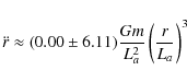
Results. The residual gravity effect occurs in all four cases. In a perfectly regular 3-torus of side length La, and in the octahedral and truncated cube spaces, the highest order term in the residual acceleration is the third-order term in the Taylor expansion in powers of r/La (3-torus), or
![]() ,
respectively. However, the Poincaré dodecahedral space is unique among the four spaces. The third order cancels, leaving the fifth order term
,
respectively. However, the Poincaré dodecahedral space is unique among the four spaces. The third order cancels, leaving the fifth order term
![]() as the most significant.
Conclusions. Not only are three of the four perfectly regular well-proportioned spaces better balanced than most other multiply connected spaces in terms of the residual gravity acceleration effect by a factor of about a million (setting
as the most significant.
Conclusions. Not only are three of the four perfectly regular well-proportioned spaces better balanced than most other multiply connected spaces in terms of the residual gravity acceleration effect by a factor of about a million (setting
![]() ), but the fourth of these spaces is about ten thousand times better balanced than the other three. This is the Poincaré dodecahedral space. Is this unique dynamical property of the Poincaré space a clue towards a theory of cosmic topology?
), but the fourth of these spaces is about ten thousand times better balanced than the other three. This is the Poincaré dodecahedral space. Is this unique dynamical property of the Poincaré space a clue towards a theory of cosmic topology?
Key words: cosmology: theory - cosmological parameters - large-scale structure of Universe - early Universe
1 Introduction
It has been shown that for zero curvature, the global topology of comoving space can affect the dynamics expected in the weak-field Newtonian limit (Roukema et al. 2007), in contrast to what was previously thought. In particular, a test particle of negligible mass near a massive particle (such as a cluster of galaxies dominated by its dark matter halo) has unequal attractions to the nearest topological images of the massive particle in opposite directions, since its position is asymmetrically offset from the massive particle. This leaves a residual acceleration effect that is qualititatively similar to that of dark energy. For realistic physical scales at the present epoch, the effect was estimated to be about 10-9 times weaker than the observed cosmological constant.
The heuristic calculations presented in Roukema et al. (2007) only considered the flat spaces
![]() and T3. However, there has been interest in the Poincaré dodecahedral space, S3/I*, being a candidate model for comoving space that explains the ``missing fluctuations problem'' tentatively observed in the COsmic Microwave Background (COBE) all-sky maps and confirmed in the Wilkinson Microwave Anisotropy Probe (WMAP) all-sky maps (Spergel et al. 2003; Luminet et al. 2003; Roukema et al. 2004; Aurich et al. 2005a,b; Gundermann 2005; Key et al. 2007; Niarchou & Jaffe 2007; Caillerie et al. 2007; Lew & Roukema 2008; Roukema et al. 2008a,b). Does a similar residual gravity effect occur in the case of positively curved space, in particular, in the Poincaré space?
and T3. However, there has been interest in the Poincaré dodecahedral space, S3/I*, being a candidate model for comoving space that explains the ``missing fluctuations problem'' tentatively observed in the COsmic Microwave Background (COBE) all-sky maps and confirmed in the Wilkinson Microwave Anisotropy Probe (WMAP) all-sky maps (Spergel et al. 2003; Luminet et al. 2003; Roukema et al. 2004; Aurich et al. 2005a,b; Gundermann 2005; Key et al. 2007; Niarchou & Jaffe 2007; Caillerie et al. 2007; Lew & Roukema 2008; Roukema et al. 2008a,b). Does a similar residual gravity effect occur in the case of positively curved space, in particular, in the Poincaré space?
An additional question of interest is whether or not the residual gravity effect might distinguish the Poincaré space from other well-proportioned spaces (Weeks et al. 2004). The Poincaré space is presently preferred to the octahedral space (S3/T*) and the truncated cube space (S3/O*) because of empirical constraints on curvature. For a total density of
![]() ,
the latter two spaces have larger fundamental domains than the Poincaré space and so have difficulty explaining the missing fluctuations problem. However, this is an empirical argument with no theoretical motivation. Could there be any dynamical arguments either favouring or disfavouring the Poincaré space? Some steps have been taken towards what might develop into a quantum cosmology theory of cosmic topology, using various notions of distance between different manifolds (Masafumi 1996; Anderson et al. 2004) and analysis of topology change in quantum gravity (e.g., Dowker & Surya 1998). The residual gravity effect might contribute an additional criterion for comparing different manifolds.
,
the latter two spaces have larger fundamental domains than the Poincaré space and so have difficulty explaining the missing fluctuations problem. However, this is an empirical argument with no theoretical motivation. Could there be any dynamical arguments either favouring or disfavouring the Poincaré space? Some steps have been taken towards what might develop into a quantum cosmology theory of cosmic topology, using various notions of distance between different manifolds (Masafumi 1996; Anderson et al. 2004) and analysis of topology change in quantum gravity (e.g., Dowker & Surya 1998). The residual gravity effect might contribute an additional criterion for comparing different manifolds.
Here, the residual gravity effect in the octahedral space, the truncated cube space, and the Poincaré space is studied by considering the dynamics of a negligible-mass test particle near a
massive particle. As in Roukema et al. (2007), this approach can be considered as an heuristic model for a positively curved space that is homogeneous except for a small neighbourhood around one point, in which a positive density fluctuation of matter has collapsed into a high-density, nearly point-like object, in excess of the underlying homogeneous density distribution. To satisfy Stokes' theorem, the weak-limit gravitational attraction in the three spherical spaces is set to be proportional to
![\begin{displaymath}%
\left[ R_{{\rm C}}\sin\left(\frac{r}{R_{{\rm C}}}\right) \right]^{-2}
\end{displaymath}](/articles/aa/full_html/2009/28/aa11881-09/img17.png)
rather than r-2 (see Sect. 2.1), where
The method is described in more detail in Sect. 2. Residual accelerations estimated to the third order in the Taylor expansion of the fractional displacement are presented for the 3-torus
in Sect. 3.1. Residual accelerations to fifth order for individual pairs of opposite images in the spherical spaces are presented analytically in Sect. 3.2. Residual accelerations to fifth order for the full set of adjacent![]() images in the spherical spaces are presented numerically in Sect. 3.3. For the Poincaré space, an analytical derivation of the residual acceleration to fifth order is also given in Sect. 3.3.1. A statistical summary is presented in Sect. 3.3.2.
images in the spherical spaces are presented numerically in Sect. 3.3. For the Poincaré space, an analytical derivation of the residual acceleration to fifth order is also given in Sect. 3.3.1. A statistical summary is presented in Sect. 3.3.2.
Discussion and conclusions are given in Sects. 4 and 5 respectively. Discussion of spherical, multiply connected spaces is available in Weeks (2001), Gausmann et al. (2001), Lehoucq et al. (2002), and Riazuelo et al. (2004), and we refer the reader to references therein for introductions to cosmic topology. Distances are calculated in a spatial section at constant cosmological time in the universal covering space (S3 for the spherical spaces,
![]() for T3), by default as ``physical'' distances, i.e.,
for T3), by default as ``physical'' distances, i.e., ![]() ,
where a(t) is the scale factor and
,
where a(t) is the scale factor and ![]() is a comoving distance (i.e.
is a comoving distance (i.e. ![]() is a ``proper distance'' at the present epoch (Weinberg 1972), equivalent to ``conformal time'' if c=1). Distance units are normally presented here in
is a ``proper distance'' at the present epoch (Weinberg 1972), equivalent to ``conformal time'' if c=1). Distance units are normally presented here in
![]() or
or
![]() ,
where the Hubble constant is written
,
where the Hubble constant is written
![]() km s-1 Mpc1. The fundamental domains of all the spaces are assumed to be perfectly regular. The Newtonian gravitational constant is written as G.
km s-1 Mpc1. The fundamental domains of all the spaces are assumed to be perfectly regular. The Newtonian gravitational constant is written as G.
2 Method
Although dynamics in the Poincaré dodecahedral space S3/I* could, in principle, be studied by applying boundary conditions that identify opposite faces of a dodecahedral fundamental domain of a positive curvature radius
![]() with one another, this would probably be extremely complicated for both analytical and numerical calculations. It is simpler to work in the universal covering space S3 represented as a subspace of
with one another, this would probably be extremely complicated for both analytical and numerical calculations. It is simpler to work in the universal covering space S3 represented as a subspace of
![]() .
.
As described in Sect. 2.1 of Roukema et al. (2007), several assumptions are required for this heuristic approach. Here, the corresponding assumptions are as follows:
- (1)
- the flat Newtonian approximation of gravity is replaced by the equivalent in positively curved space, as described in Eq. (1) above;
- (2), (3)
- the covering space is S3, which is not flat;
- (4)
- a finite particle horizon
 that is just large enough to include all adjacent topological images is assumed;
- (5), (6)
- identical to those in Roukema et al. (2007): the metric is assumed to be that for a perfectly homogeneous model of the same curvature, except that the distant, multiple copies of the local massive particle are considered to provide a contribution to the local gravitational potential that may not fully cancel;
- (7), (8)
- are not needed here since the one-body problem in S3 (Sect. 3.1.1, Roukema et al.) is divergent and only briefly mentioned in Sect. 2.1.
2.1 Weak-limit gravity and divergences
As stated in Eq. (1), to satisfy Stokes' theorem, the weak-limit gravitational attraction towards a single massive particle is set to be proportional to
![]() rather than r-2. This can be understood as follows.
rather than r-2. This can be understood as follows.
Let S3 be represented by a spherical coordinate system centred on the massive particle, so that the Friedmann-Lemaître-Robertson-Walker (FLRW) line element is written
| (2) |
where the scale factor a(t) is subsumed into r and
| (3) |
by symmetry, where
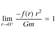
in order to agree with the flat-space Newtonian limit towards the massive particle of mass m. Let V be the interior of a 2-sphere of radius r centred at the massive particle. Applying Stokes' theorem to
using the FLRW metric. Since the only source of the vector field
using Eqs. (5) and (4) respectively. Equating the right-hand sides of Eqs. (5) and (6) gives the weak limit acceleration induced by a single massive particle in a positively curved space of radius
![\begin{displaymath}%
\ddot{\vec{r}} = f(r) \; \hat{\vec{r}} = -\frac{G m \;
\hat{\vec{r}} } {[R_{{\rm C}}\sin(r/R_{{\rm C}})]^2}\cdot
\end{displaymath}](/articles/aa/full_html/2009/28/aa11881-09/img40.png)
For instantaneous transmission of gravitational signals in an infinitely old, static, simply connected space, this implies two divergence problems.
Firstly, a single massive point particle of mass m in a perfectly uniform and otherwise empty S3 yields an infinite repulsive force at the antipode of the massive particle, since
![]() .
More generally, an infinite repulsive (attractive) force exists for gravitational signals that have travelled odd (even) values of j times the half-circumference
.
More generally, an infinite repulsive (attractive) force exists for gravitational signals that have travelled odd (even) values of j times the half-circumference
![]() from the massive object, i.e. j/2 times around the whole space, where
from the massive object, i.e. j/2 times around the whole space, where
![]() .
.
Secondly, even if we ignore the model of a zero-size point particle as an idealised fiction, a problem remains for a negligible-mass test particle near a massive particle. The test particle
also experiences accelerations from signals that have travelled j times around S3 in the two different directions along the great circle passing through the test particle and the massive particle, where
![]() .
This second divergence problem is similar to the divergence problem in flat, simply connected, infinitely sized, infinitely old, Newtonian space with instantaneous transmission of the gravitational signal. The total acceleration towards the massive particle would be
.
This second divergence problem is similar to the divergence problem in flat, simply connected, infinitely sized, infinitely old, Newtonian space with instantaneous transmission of the gravitational signal. The total acceleration towards the massive particle would be
which is clearly divergent.
The former divergence, i.e., the
![]() singularity related to the zero size of the massive point particle and the nature of positive curvature, is clearly unphysical if we are interested in
a smoothing length on the scale of a galaxy cluster. The latter divergence, i.e. that in Eq. (8), is removed by assumption (4) above. Assumption (4) also removes the
singularity related to the zero size of the massive point particle and the nature of positive curvature, is clearly unphysical if we are interested in
a smoothing length on the scale of a galaxy cluster. The latter divergence, i.e. that in Eq. (8), is removed by assumption (4) above. Assumption (4) also removes the
![]() divergence. A finite particle horizon
divergence. A finite particle horizon
![]() just large enough to include the adjacent topological images is necessary for a residual gravity effect to occur, but it does not need to
be as large as
just large enough to include the adjacent topological images is necessary for a residual gravity effect to occur, but it does not need to
be as large as
![]() .
The adjacent topological images in S3/T*, S3/O*, and
S3/I* are at
.
The adjacent topological images in S3/T*, S3/O*, and
S3/I* are at
![]() ,
,
![]() and
and
![]() ,
and
,
and
![]() respectively.
Moreover, observationally realistic estimates of the total density parameter
respectively.
Moreover, observationally realistic estimates of the total density parameter![]() are consistent with the range that is empirically interesting for the Poincaré space,
are consistent with the range that is empirically interesting for the Poincaré space,
![]() .
The range
.
The range
![]() corresponds to a curvature radius of
corresponds to a curvature radius of
![]() respectively. Hence, for the three well-proportioned, spherical spaces, the appropriate horizon distances for the arrival of gravitational signals from the adjacent topological images are in the range
respectively. Hence, for the three well-proportioned, spherical spaces, the appropriate horizon distances for the arrival of gravitational signals from the adjacent topological images are in the range
![]() ,
i.e. up to a few times the distance to the surface of last scattering
,
i.e. up to a few times the distance to the surface of last scattering
![]() .
As noted in Roukema et al. (2007), a moderate amount of inflation in the early Universe could be one way of satisfying assumption (4).
.
As noted in Roukema et al. (2007), a moderate amount of inflation in the early Universe could be one way of satisfying assumption (4).
2.2 Residual gravity
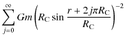
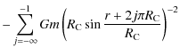
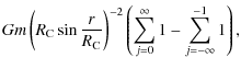
The weak-limit residual acceleration on a test particle at ![]() near the massive particle of mass m at 0 can be written
near the massive particle of mass m at 0 can be written
![$\displaystyle %
\ddot{\vec{r}} =
\sum_{j=1,d_j \equiv a\chi[\vec{r},g_j({0})] }...
... m \left( R_{{\rm C}}\sin \frac{d_j}{R_{{\rm C}}} \right)^{-2}
\hat{\vec{r}}_j,$](/articles/aa/full_html/2009/28/aa11881-09/img59.png)
where
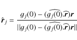
where
![$\displaystyle %
\left( \sin \frac{d_j}{R_{{\rm C}}} \right)^{-2} =
\left( \sin ...
...\left\{ 1-
\left[ \widehat{g_j({0})}. \widehat{\vec{r}}\right]^2 \right\}^{-1}.$](/articles/aa/full_html/2009/28/aa11881-09/img69.png)
The curvature is set to
2.3 Numerical precision
For the full set of adjacent topological images in the spherical spaces, Eq. (9) is evaluated primarily by a numerical approach, using double precision floating-point operations where sufficient, and arbitrary precision floating-point operations where necessary. Typical scales of interest, i.e., for typical test particles in a void of large-scale structure, are a few tens of megaparsecs. This gives
![]() as a useful domain for finding the highest terms in the Taylor expansion of the residual gravity
for
as a useful domain for finding the highest terms in the Taylor expansion of the residual gravity
for
![]() ,
where
,
where
![]() as stated above. By setting
as stated above. By setting
![]() internally in numerical calculations, nearly equal and opposite accelerations from nearly opposed topological images are each of approximately unity order, the fourth and fifth order terms at the lower limit
internally in numerical calculations, nearly equal and opposite accelerations from nearly opposed topological images are each of approximately unity order, the fourth and fifth order terms at the lower limit
![]() should therefore be above the numerical noise limit, if the calculating precision is well below
should therefore be above the numerical noise limit, if the calculating precision is well below
![]() and 10-20, respectively. These would require precision in the significand
and 10-20, respectively. These would require precision in the significand![]() well above
well above
![]() and
and
![]() bits respectively. According to the IEEE 754-1985 standard, double-precision floating-point numbers have 53-bit precision in the significand (including one implicit bit). This would at best provide just one bit of information for a fourth order term and no information for a fifth order term for
bits respectively. According to the IEEE 754-1985 standard, double-precision floating-point numbers have 53-bit precision in the significand (including one implicit bit). This would at best provide just one bit of information for a fourth order term and no information for a fifth order term for
![]() .
For this reason, an arbitrary precision library is used here to examine higher
order terms.
.
For this reason, an arbitrary precision library is used here to examine higher
order terms.
Analytical calculations are also made for the Poincaré space. We also revisit the T3 calculation made in Sect. 3.2 of Roukema et al. (2007), in order to consider higher order terms. The first order term was found to cancel for a perfectly regular T3 model.
3 Results
3.1 T3 revisited
In Sect. 3.2 of Roukema et al. (2007), an analytical estimate of the acceleration from all six adjacent images in a T3 model was shown to be zero to first order when the three fundamental lengths of the model are exactly equal. However, the lower scatterings of points in Figs. 7 and 8 of that paper do not represent numerical error. Recalculation of Eqs. (11) to (15) of Roukema et al. (2007) to higher order shows that for perfectly equal fundamental lengths La = Le = Lu, higher order terms in Eq. (15) do not all cancel. The lowest order non-cancelling terms are the third order terms
where the massive particle is at the origin (0,0,0) in the covering space
and a skewness
for convenience.
![\begin{figure}
\par\includegraphics[width=8cm,clip]{1881fig1.eps}
\end{figure}](/articles/aa/full_html/2009/28/aa11881-09/img90.png) |
Figure 1:
Residual acceleration (radial component) induced on a test particle near a massive particle such as a cluster of galaxies by the six adjacent topological images of the massive particle, in a T3 universe of three exactly comoving equal side lengths La. The accelerations a3(r) are normalised to be constant if the dominant term is third order in r/La (see Eq. (14)) and are shown against distance
r < 0.01 La from the massive particle, where
|
| Open with DEXTER | |
The analytical and numerical calculations are clearly consistent in showing that in the case of perfectly equal fundamental side lengths of a T3 model, there is indeed a residual topological gravity effect. The residual acceleration is anisotropic, depending on the relation between the test particle's displacement from the massive particle and the orientation of the fundamental directions. The positive skewness implies that even though the mean radial acceleration is close to zero, the mode and median are negative, i.e., test particles placed in random directions relative to the massive particle are more likely to be subject to a radial deceleration rather than a radial acceleration. The amplitude of the effect is third order, i.e., about (r/La)2 times smaller than the residual effect that occurs for slightly unequal fundamental lengths. If an upper estimate for r/La at the present epoch is used, then this is a factor of about a million.
3.2 One pair of opposite topological images in S

Before considering the full effect from a layer of topological images in the spherical cases,
let us first consider the effect of just one pair of opposite topological images of the ``local'' massive particle. This is somewhat similar to the
![]() case considered in Sect. 3.1.1 of Roukema et al. (2007), where the test particle lies along the geodesic joining the three images of the massive particle to one another in one of the spherical spaces, i.e.,
case considered in Sect. 3.1.1 of Roukema et al. (2007), where the test particle lies along the geodesic joining the three images of the massive particle to one another in one of the spherical spaces, i.e.,
![]() for an appropriate holonomy group
for an appropriate holonomy group ![]() .
This may help us to understand the full sum from all the adjacent images. Similarly to Eq. (2) of Roukema et al. (2007), we can use scalar quantities. The acceleration to fifth order in
.
This may help us to understand the full sum from all the adjacent images. Similarly to Eq. (2) of Roukema et al. (2007), we can use scalar quantities. The acceleration to fifth order in
![]() for the Poincaré space is
for the Poincaré space is![]()
![$\displaystyle G \frac{m}{R_{{\rm C}}^2}
\left\{
\left[ \sin \left(\frac{\pi}{5}...
...[ \sin \left(\frac{\pi}{5} + \frac{r}{R_{{\rm C}}} \right)\right]^{-2}
\right\}$](/articles/aa/full_html/2009/28/aa11881-09/img93.png)
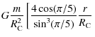
![$\displaystyle + \left. \frac{16\cos(\pi/5)\sin^2(\pi/5)+24\cos^3(\pi/5)}{3\sin^5(\pi/5)}
\left(\frac{r}{R_{{\rm C}}} \right)^3 + \ldots \right]$](/articles/aa/full_html/2009/28/aa11881-09/img95.png)
![$\displaystyle G \frac{m}{R_{{\rm C}}^2} \left[ 15.9 \left(\frac{r}{R_{{\rm C}}}...
...}}} \right)^3 +
310.4 \left(\frac{r}{R_{{\rm C}}} \right)^5 + \ldots \right].~~$](/articles/aa/full_html/2009/28/aa11881-09/img97.png)
This is similar to the flat case. The residual acceleration is proportional to the displacement to first order, which again is behaviour similar to that of a cosmological constant:
The octahedral space has adjacent images at
![$\displaystyle G \frac{m}{R_{{\rm C}}^2} \left\{
\left[ \sin \left(\frac{\pi}{3}...
...[ \sin \left(\frac{\pi}{3} + \frac{r}{R_{{\rm C}}} \right)\right]^{-2}
\right\}$](/articles/aa/full_html/2009/28/aa11881-09/img99.png)
![$\displaystyle \frac{16\sqrt{3}}{9} G \frac{m}{R_{{\rm C}}^2}
\left[
\frac{r}{R_...
...\right)^3 +
\frac{14}{5} \left(\frac{r}{R_{{\rm C}}} \right)^5 +
\ldots \right]$](/articles/aa/full_html/2009/28/aa11881-09/img100.png)
![$\displaystyle G \frac{m}{R_{{\rm C}}^2}
\left[ 3.1 \left(\frac{r}{R_{{\rm C}}} ...
...rm C}}} \right)^3 +
8.6 \left(\frac{r}{R_{{\rm C}}} \right)^5 +
\ldots \right].$](/articles/aa/full_html/2009/28/aa11881-09/img101.png)
Equation (17) is also valid for the adjacent images at the eight truncated corners of the fundamental domain in a truncated cube space, which are at
![$\displaystyle G \frac{m}{R_{{\rm C}}^2} \left\{
\left[ \sin \left(\frac{\pi}{4}...
...[ \sin \left(\frac{\pi}{4} + \frac{r}{R_{{\rm C}}} \right)\right]^{-2}
\right\}$](/articles/aa/full_html/2009/28/aa11881-09/img102.png)
![$\displaystyle 8 G \frac{m}{R_{{\rm C}}^2}
\left[
\frac{r}{R_{{\rm C}}} +
\frac{...
...ight)^3 +
\frac{122}{15} \left(\frac{r}{R_{{\rm C}}} \right)^5 +
\ldots \right]$](/articles/aa/full_html/2009/28/aa11881-09/img103.png)
![$\displaystyle G \frac{m}{R_{{\rm C}}^2}
\left[ 8 \left(\frac{r}{R_{{\rm C}}} \r...
...m C}}} \right)^3 +
65.1 \left(\frac{r}{R_{{\rm C}}} \right)^5 +
\ldots \right].$](/articles/aa/full_html/2009/28/aa11881-09/img104.png)
Each of these calculations is for just one pair of topological images adjacent to the ``local'' copy of the massive particle, lying in opposite directions. In the flat case, this can be thought of as a
On the other hand, Eqs. (15), (17), and (18) hint at the form that numerical estimates for the sum of the weak-limit residual gravitational effect from all the adjacent images may take for a given spherical
manifold. For
S3/I*, the full set of adjacent images of the massive particle consists of six pairs of images. For a test particle displaced slightly in a random direction from the massive particle, the two images in a pair will be seen in nearly, although not exactly, opposite directions in the tangent 3-space at the test particle's location at
![]() .
The modulus of the (vector) residual acceleration induced by the nearly opposite pair should not be very different from the expression given in Eq. (15), although its expression using elementary algebra might appear complicated.
.
The modulus of the (vector) residual acceleration induced by the nearly opposite pair should not be very different from the expression given in Eq. (15), although its expression using elementary algebra might appear complicated.
This suggests that the scalar amplitude of the vector sum of all twelve accelerations is likely to involve terms of first, third, and fifth order in
![]() ,
with coefficients of the order of magnitude of those in Eq. (15). However, this argument is not exact. A test particle displaced from the massive particle in an arbitrary direction does not, in general, lie
along the great circle defined by a given pair of opposite images, and can at most lie along only one of the great circles defined by the six pairs of opposite images. Hence, terms with even powers of
,
with coefficients of the order of magnitude of those in Eq. (15). However, this argument is not exact. A test particle displaced from the massive particle in an arbitrary direction does not, in general, lie
along the great circle defined by a given pair of opposite images, and can at most lie along only one of the great circles defined by the six pairs of opposite images. Hence, terms with even powers of
![]() could also appear in the Taylor expansion.
could also appear in the Taylor expansion.
These single-pair calculations might also be of interest for ill-proportioned (Weeks et al. 2004) positively curved spaces, e.g., the lens spaces L(p,q), with
![]() relatively prime, where
relatively prime, where ![]() (e.g. Sect. 4, Gausmann et al. 2001). Since these spaces are not globally homogeneous, derivations similar to those in Eqs. (15), (17), and (18) would be strictly valid only for points lying along the symmetry axis joining the centres of the two faces of the fundamental dihedron (lens), i.e., where adjacent topological images are separated by a spatial geodesic of length
(e.g. Sect. 4, Gausmann et al. 2001). Since these spaces are not globally homogeneous, derivations similar to those in Eqs. (15), (17), and (18) would be strictly valid only for points lying along the symmetry axis joining the centres of the two faces of the fundamental dihedron (lens), i.e., where adjacent topological images are separated by a spatial geodesic of length
![]() .
This direction would therefore be unstable to a linear-term acceleration effect that would tend to expand it faster than other directions. This is qualitatively similar to the effect found in Sect. 3 of Roukema et al. (2007), according to which the residual acceleration would tend to equalise the three fundamental lengths of a T3 model of slightly unequal fundamental lengths.
.
This direction would therefore be unstable to a linear-term acceleration effect that would tend to expand it faster than other directions. This is qualitatively similar to the effect found in Sect. 3 of Roukema et al. (2007), according to which the residual acceleration would tend to equalise the three fundamental lengths of a T3 model of slightly unequal fundamental lengths.
![\begin{figure}
\par\includegraphics[width=8cm,clip]{1881fig2.eps}
\end{figure}](/articles/aa/full_html/2009/28/aa11881-09/img110.png) |
Figure 2:
Residual acceleration (radial component) induced on a test particle
near a massive particle by the eight adjacent topological images of the massive particle,
in a universe whose 3-manifold of comoving space is the octahedral space S3/T*. The accelerations a3(r) are normalised to be constant if the dominant term is third order in r/La(see Eq. (19)) and are shown against distance
|
| Open with DEXTER | |
3.3 Well-proportioned spherical spaces: S3/T*, S3/O*, and S3/I*
As described in Sects. 2.2 and 2.3, for a test particle at ![]() in S3/T*, S3/O*, or
S3/I*, let us set
in S3/T*, S3/O*, or
S3/I*, let us set
![]() ,
,
![]() ,
or
,
or
![]() ,
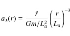
respectively. Equation (9) is evaluated numerically for 200 randomly (logarithmically) distributed test particles at distances of up to 250 h-1 Mpc from the massive particle. Figures 2-4 show
the residual accelerations, scaled by
,
respectively. Equation (9) is evaluated numerically for 200 randomly (logarithmically) distributed test particles at distances of up to 250 h-1 Mpc from the massive particle. Figures 2-4 show
the residual accelerations, scaled by
![]() so that they should be approximately constant
if the dominating term in
so that they should be approximately constant
if the dominating term in
![]() is the third order term, i.e.,
is the third order term, i.e.,
is shown.
It is clear that both the octahedral and truncated cube spaces have similar Taylor series behaviour to that of T3. The linear term cancels, but a third-order-dominated residual acceleration
remains. On the other hand, it is clear from Fig. 4 that the Poincaré dodecahedral space has a residual acceleration that is much weaker than those of the other three spaces, and that this is poorly modelled as a third order term in
![]() .
Instead, the constant slope of the relation in Fig. 4 strongly suggests that the residual acceleration for the Poincaré space is dominated by a fifth order term, i.e.,
.
Instead, the constant slope of the relation in Fig. 4 strongly suggests that the residual acceleration for the Poincaré space is dominated by a fifth order term, i.e.,
is approximately constant and terms lower than the fifth order cancel.
![\begin{figure}
\par\includegraphics[width=8cm,clip]{1881fig3.eps}
\end{figure}](/articles/aa/full_html/2009/28/aa11881-09/img115.png) |
Figure 3: As for Fig. 2, for the truncated cube space S3/O*. |
| Open with DEXTER | |
![\begin{figure}
\includegraphics[width=8cm,clip]{1881fig4.eps}
\end{figure}](/articles/aa/full_html/2009/28/aa11881-09/img116.png) |
Figure 4: Residual acceleration (radial component), as for Fig. 2, for the Poincaré dodecahedral space S3/I*. |
| Open with DEXTER | |
The remaining orthogonal component of the residual acceleration is of a similar order of magnitude to that of the radial component. Figure 5 shows that provided that the component is calculated with at least 70-bit precision in the significand, it is dominated by the
![]() term.
term.
The previous figures were calculated using 70-bit significand multi-precision floating-point operations. The effect of reducing the precision to 50 or 60 bits is clear in Fig. 5, i.e., for the orthogonal component of the residual
acceleration in the Poincaré space. Noise created by the precision limit enters the
calculation, for example, when converting from a double-precision position in
![]() of
the test particle to a multi-precision position. Apart from special cases, the finite precision
representation of a typical, pseudo-random particle position in
of
the test particle to a multi-precision position. Apart from special cases, the finite precision
representation of a typical, pseudo-random particle position in
![]() will place the particle at a position slightly offset from the physical 3-surface S3, because of the limited precision. If the particle is not located exactly on S3, then this induces an acceleration that is orthogonal to the tangent 3-plane at
will place the particle at a position slightly offset from the physical 3-surface S3, because of the limited precision. If the particle is not located exactly on S3, then this induces an acceleration that is orthogonal to the tangent 3-plane at ![]() .
The numerical noise component appears on the left of Fig. 5 as a constant value of
.
The numerical noise component appears on the left of Fig. 5 as a constant value of ![]() ,
i.e.,
,
i.e.,
![]() .
.
![\begin{figure}
\par\includegraphics[width=8cm,clip]{1881fig5.eps}
\end{figure}](/articles/aa/full_html/2009/28/aa11881-09/img120.png) |
Figure 5:
Orthogonal residual acceleration for the Poincaré dodecahedral space
S3/I*, as for Fig. 4, shown using 50-bit ( |
| Open with DEXTER | |
3.3.1 Analytical estimate for the Poincaré space
Analytical evaluation of Eq. (9) to fifth order for the Poincaré
dodecahedral space using a computer algebra system![]() confirms the numerical estimates shown in Figs. 4 and 5. The highest order residual acceleration from the adjacent topological images is
confirms the numerical estimates shown in Figs. 4 and 5. The highest order residual acceleration from the adjacent topological images is

where the massive particle is at (0,0,0,1), the test particle displaced from it in an arbitrary direction by a small amount is located at
| |
|||
| -6744.5 x2 -10912.8 y2 + 2224.7) x, | |||
| (4304.3 y4 +7540.5 z4 +17657.2 y2 z2 | |||
| -6744.5 y2 -10912.8 z2 + 2224.7) y, | |||
| (4304.3 z4 +7540.5 x4 +17657.2 z2 x2 | |||
| -6744.5 z2 -10912.8 x2 + 2224.7) z, 0]. | (22) |
The radial and orthogonal components of the residual acceleration can now be calculated as follows. Firstly, a small numerical value
3.3.2 Statistical description
For an isotropic distribution of the directions of displacement of the test particle, Table 1 lists characteristic statistics of the radial and orthogonal components of the
residual acceleration for the four well-proportioned spaces, primarily calculated from direct numerical estimates using Eq. (9). By construction, the orthogonal component is necessarily non-negative. Since estimation of the parameters of the Poincaré space residual acceleration is sensitive to numerical precision limits, Table 1 also lists parameters for the Poincaré space radial component estimated using Eq. (21) and the unit tangent vector described above. Within the uncertainties indicated by the standard error in the mean
![]() ,
the two estimates agree.
,
the two estimates agree.
Table 1:
Statistical characteristics of coefficients ai of the dominant (ith order) term in the radial and orthogonal components of the residual acceleration ![]() in perfectly regular well-proportioned spaces, for approximately isotropic displacements
in perfectly regular well-proportioned spaces, for approximately isotropic displacements ![]() a.
a.
4 Discussion
The results shown above are quite sensitive to small errors in the positions of the adjacent topological images. This provides a useful check of the calculations, since a small arbitrary error is most likely to yield a stronger residual acceleration than a weaker one. Increasing or decreasing the distances from the massive particle to the two members of one of the opposite pairs of topological images by ![]() is sufficient to destabilise the nearly perfect equilibrium defined by the full set of adjacent topological images for a given space. The residual acceleration reverts to being dominated by
is sufficient to destabilise the nearly perfect equilibrium defined by the full set of adjacent topological images for a given space. The residual acceleration reverts to being dominated by
![]() rather than
rather than
![]() or
or
![]() .
.
This sensitivity to small changes in the distances to topological images is physically interesting. As found in Sect. 3 of Roukema et al. (2007), the residual acceleration in a T3 model of slightly unequal fundamental lengths is dominated by a linear term in r/La, which tends to equalise the three fundamental lengths. The same relation applies for the spherical models. These are very well balanced in the sense that the linear term cancels, and in the case of the Poincaré space, the cubic term cancels too, provided that these spaces are perfectly homogeneous. A small decrease in the injectivity diameter in one direction implies stronger acceleration for a test particle, favouring a return towards perfect isotropy in the fundamental lengths. Conversely, a small increase in the injectivity diameter implies weaker acceleration, again favouring a return towards isotropy. The residual acceleration tends to encourage the space to return to perfect ``residual acceleration equilibrium'', in which the residual acceleration disappears down to the third or fifth order.
Clearly, these effects are negligible in the present epoch at the level of observational detectability for the next few decades. Moreover, given the present empirical interest in the Poincaré space, the prediction of the perfectly isotropic model would be an absence of a residual acceleration effect to a much higher observational accuracy than that for the effects predicted by the other three well-proportioned models, which in turn would be more difficult to detect than the residual acceleration effect from ill-proportioned models.
However, the Universe is certainly inhomogeneous. If evidence continues to accumulate for the Poincaré space model with successively more accurate estimates of the model's astronomical coordinates, following the estimates made in Roukema et al. (2008a,b), then several observational approaches could be used to test the predictions of the residual acceleration effect. With a sufficient level of precision, matched circles and/or annuli on the sky should yield slightly different fundamental lengths along the six axes. The residual acceleration effect should consist of a positive or negative extra acceleration for shorter or longer fundamental lengths, respectively. Surveys of tracers of large-scale structure lying along the different geodesics to topological images of, for example, the Virgo cluster, could also be used to estimate which directions should have slightly longer than average geodesics and which should have slightly shorter than average geodesics. All three estimates should agree with one another, provided that no other sources of random and systematic error interfere. Hence, the residual acceleration effect potentially offers a physical mechanism for testing a multiply-connected model of comoving space, as an alternative to relying on geometrical effects (individual or statistical identification of multiply imaged objects or regions of space).
Another interesting question is whether or not the better ``balancing'' of the Poincaré space could have had any role in the evolution of a preferred topology in the early Universe, especially during the quantum epoch. Does the Poincaré space occupy a dynamically more stable state than the other well-proportioned spaces, which in turn are more stable than ill-proportioned spaces? This would most likely require significant inhomogeneities in the very early Universe, which themselves might have been subsequently removed by the residual gravity acceleration effect itself.
Apart from the possible physical consequences of this result, it may be interesting to ask if these results are reasonable from an intuitive mathematical point of view. It is useful to consider this in terms of pairs of opposite images, since if the test particle lies along the geodesic joining the local copy and the two opposite distant copies of the massive particle, then the single pair yields a linear-dominated residual acceleration. In order for the linear (or higher order) terms in the residual acceleration to cancel, the acceleration components that are approximately orthogonal to the geodesic joining the test particle to the two members of a given opposite pair need to be able to cancel the approximately radial components of residual accelerations in other pairs of images. In the T3 case, three nearly orthogonal pairs are sufficient for the linear terms to completely cancel in this way (provided that the fundamental domain is perfectly regular). Given that S3/T*, S3/O*, and S3/I* have four, seven, and six opposite pairs, respectively, it is reasonable to imagine that the radial components of the linear residual-acceleration term of a given pair are cancelled by the orthogonal components of the other pairs, since there are many of them, distributed symmetrically.
It is also possible to imagine that with a high enough number of opposite pairs and sufficient symmetry, a higher order term such as the third order might also disappear, by means of fine balancing between the different directions. The truncated cube space S3/O* and the Poincaré space S3/I* have the highest numbers of opposite pairs, or equivalently, the highest numbers of pairs of faces of their fundamental domains. However, the truncated cube cannot be a regular polyhedron; its faces are six truncated squares and eight triangles. All the faces of the fundamental domain of the Poincaré dodecahedral space have the same shape: a pentagon. In this sense, it is more symmetrical than the truncated cube space. So requiring both a fundamental domain with a high number of faces and a high level of symmetry would seem to provide a qualitative pair of conditions to explain why the Poincaré space is more finely balanced than the other well-proportioned spaces.
However, could either the subset of topological images corresponding to only the octagonal faces of the fundamental domain of the truncated cube, or the subset corresponding to only the triangular faces, nevertheless cancel to fifth order, and become hidden because the other subset reintroduces a third order term? A calculation similar to those developed above shows that both subsets separately retain the third order as the dominant order. Table 2 gives statistical characteristics of the third order coefficients for the two subsets. So the Poincaré space retains its uniqueness in cancelling down to fifth order.
Table 2:
Components of the residual acceleration ![]() ,
as for Table 1, for the truncated cube space, separated by fundamental domain face shape.
,
as for Table 1, for the truncated cube space, separated by fundamental domain face shape.
An aspect of the residual acceleration as expressed in Eqs. (21) and (22) that may initially seem counterintuitive is the permutational symmetry between the x,y, and z components, since a dodecahedron is not always thought of as having cubical symmetry. However, an appropriate orientation of the dodecahedron in
![]() ,
such as that used in our computer algebra script, shows an (x,y,z) symmetry. The twelve adjacent
topological images consist of three quadruplets orthogonally projected to
,
such as that used in our computer algebra script, shows an (x,y,z) symmetry. The twelve adjacent
topological images consist of three quadruplets orthogonally projected to
![]() ,
,
![]() ,
,
![]() ,
and
,
and
![]() .
Each of these quadruplets lies in a 2-plane in
.
Each of these quadruplets lies in a 2-plane in
![]() ,
i.e., x=0, y=0, and z=0, respectively. In this orientation, the ``top'' and ``bottom'' of the dodecahedron are edges, not faces. These two edges, along with four others, can be used to inscribe the dodecahedron in a cube (in flat space).
,
i.e., x=0, y=0, and z=0, respectively. In this orientation, the ``top'' and ``bottom'' of the dodecahedron are edges, not faces. These two edges, along with four others, can be used to inscribe the dodecahedron in a cube (in flat space).
5 Conclusions
In Roukema et al. (2007), it was found that a residual gravity acceleration effect exists for
![]() but cancels to first order for a perfectly regular T3 model. Here, it was found that the residual acceleration in T3 does not completely cancel. In T3 and two
other well-proportioned spaces, the octahedral space S3/T* and the truncated cube space S3/O*, the residual acceleration exists as a third order effect in the Taylor expansions in r/La and
but cancels to first order for a perfectly regular T3 model. Here, it was found that the residual acceleration in T3 does not completely cancel. In T3 and two
other well-proportioned spaces, the octahedral space S3/T* and the truncated cube space S3/O*, the residual acceleration exists as a third order effect in the Taylor expansions in r/La and
![]() respectively. A reasonable upper limit to
respectively. A reasonable upper limit to
![]() can be set by considering test particles in voids of large-scale structure, i.e., at typically a few megaparsecs from the most massive nearby object, and an injectivity diameter for the 3-manifold of comoving space of at least a few gigaparsecs, i.e.,
can be set by considering test particles in voids of large-scale structure, i.e., at typically a few megaparsecs from the most massive nearby object, and an injectivity diameter for the 3-manifold of comoving space of at least a few gigaparsecs, i.e.,
![]() .
Hence, at the present epoch, these three well-proportioned spaces are about a million times better balanced by this dynamical criterion than ill-proportioned spaces.
.
Hence, at the present epoch, these three well-proportioned spaces are about a million times better balanced by this dynamical criterion than ill-proportioned spaces.
The Poincaré dodecahedral space S3/I*, presently a candidate 3-manifold for comoving space favoured by several observational analyses, has been found to be even more exceptional. Its residual acceleration is dominated by the fifth order term of amplitude
![]() (Figs. 4, 5, Table 1, Eqs. (21), (22)). This makes it about ten thousand times better balanced than the other three well-proportioned spaces, i.e., about 1010 times better balanced than ill-proportioned spaces. Moreover, perturbations to this equilibrium favour a return to the equilibrium state. Are these clues towards a theory of cosmic topology?
(Figs. 4, 5, Table 1, Eqs. (21), (22)). This makes it about ten thousand times better balanced than the other three well-proportioned spaces, i.e., about 1010 times better balanced than ill-proportioned spaces. Moreover, perturbations to this equilibrium favour a return to the equilibrium state. Are these clues towards a theory of cosmic topology?
Acknowledgements
Thank you to Zbigniew Bulinski and Bartosz Lew for helpful discussion and to an anonymous referee for useful suggestions. Use was made of the Centre de Données astronomiques de Strasbourg (http://cdsads.u-strasbg.fr), the computer algebra program MAXIMA, the GNU O CTAVE command-line, high-level numerical computation software (http://www.gnu.org/software/octave), the GNU multi-precision library (GMP) and the MPFR library, the GNU Scientific Library (GSL), and the GNU PLOTUTILS plotting package.
References
- Anderson, M., Carlip, S., Ratcliffe, J. G., Surya, S., & Tschantz, S. T. 2004, Class. Quant. Gra., 21, 729 [NASA ADS] [CrossRef] (In the text)
- Aurich, R., Lustig, S., & Steiner, F. 2005a, Class. Quant. Gra., 22, 3443 [NASA ADS] [CrossRef] (In the text)
- Aurich, R., Lustig, S., & Steiner, F. 2005b, Class. Quant. Gra., 22, 2061 [NASA ADS] [CrossRef]
- Caillerie, S., Lachièze-Rey, M., Luminet, J.-P., et al. 2007, A&A, 476, 691 [NASA ADS] [CrossRef] [EDP Sciences] (In the text)
- Dowker, F., & Surya, S. 1998, Phys. Rev. D, 58, 124019 [NASA ADS] [CrossRef] (In the text)
- Gausmann, E., Lehoucq, R., Luminet, J.-P., Uzan, J.-P., & Weeks, J. 2001, Class. Quant. Gra., 18, 5155 [NASA ADS] [CrossRef] (In the text)
- Gundermann, J. 2005 [arXiv:astro-ph/0503014] (In the text)
- Key, J. S., Cornish, N. J., Spergel, D. N., & Starkman, G. D. 2007, Phys. Rev. D, 75, 084034 [NASA ADS] [CrossRef] (In the text)
- Lehoucq, R., Weeks, J., Uzan, J.-P., Gausmann, E., & Luminet, J.-P. 2002, Class. Quant. Gra., 19, 4683 [NASA ADS] [CrossRef] (In the text)
- Lew, B., & Roukema, B. F. 2008, A&A, 482, 747 [NASA ADS] [CrossRef] [EDP Sciences] (In the text)
- Luminet, J., Weeks, J. R., Riazuelo, A., Lehoucq, R., & Uzan, J. 2003, Nature, 425, 593 [NASA ADS] [CrossRef] (In the text)
- Masafumi, S. 1996, Phys. Rev. D, 53, 6902 [CrossRef] (In the text)
- Niarchou, A., & Jaffe, A. 2007, Phys. Rev. Lett., 99, 081302 [NASA ADS] [CrossRef] (In the text)
- Reichardt, C. L., Ade, P. A. R., Bock, J. J., et al. 2009, ApJ, 694, 1200 [NASA ADS] [CrossRef]
- Riazuelo, A., Weeks, J., Uzan, J., Lehoucq, R., & Luminet, J. 2004, Phys. Rev. D, 69, 103518 [NASA ADS] [CrossRef] (In the text)
- Roukema, B. F., Lew, B., Cechowska, M., Marecki, A., & Bajtlik, S. 2004, A&A, 423, 821 [NASA ADS] [CrossRef] [EDP Sciences] (In the text)
- Roukema, B. F., Bajtlik, S., Biesiada, M., Szaniewska, A., & Jurkiewicz, H. 2007, A&A, 463, 861 [NASA ADS] [CrossRef] [EDP Sciences] (In the text)
- Roukema, B. F., Bulinski, Z., Szaniewska, A., & Gaudin, N. E. 2008a, A&A, 486, 55 [NASA ADS] [CrossRef] [EDP Sciences] (In the text)
- Roukema, B. F., Bulinski, Z., & Gaudin, N. E. 2008b, A&A, 492, 673 [NASA ADS] [CrossRef]
- Spergel, D. N., Verde, L., Peiris, H. V., et al. 2003, ApJS, 148, 175 [NASA ADS] [CrossRef] (In the text)
- Spergel, D. N., Bean, R., Doré, O., et al. 2007, ApJS, 170, 377 [NASA ADS] [CrossRef]
- Weeks, J. 2001, The Shape of Space, 2nd edn. (Manhattan: Marcel Dekker) (In the text)
- Weeks, J., Luminet, J.-P., Riazuelo, A., & Lehoucq, R. 2004, MNRAS, 352, 258 [NASA ADS] [CrossRef] (In the text)
- Weinberg, S. 1972, Gravitation and cosmology: Principles and applications of the general theory of relativity (New York: Wiley) (In the text)
Footnotes
- ... adjacent
![[*]](/icons/foot_motif.png)
- ``Adjacent'' is used here to refer to images in copies of the fundamental domain that share a face with the ``original'' copy of the fundamental domain.
- ... parameter
- For example,
 ,
from WMAP 3-year and Hubble Space Telescope H0 key project data,
,
from WMAP 3-year and Hubble Space Telescope H0 key project data,
 ,
from WMAP 3-year data and Supernova Legacy Survey supernovae type Ia data (Spergel et al. 2007);
,
from WMAP 3-year data and Supernova Legacy Survey supernovae type Ia data (Spergel et al. 2007);
 ,
from WMAP 3-year and Arcminute Cosmology Bolometer Array Receiver ACBAR data (Reichardt et al. 2009).
,
from WMAP 3-year and Arcminute Cosmology Bolometer Array Receiver ACBAR data (Reichardt et al. 2009).
- ... significand
- The IEEE 754-2008 standard recommends the term ``significand'' rather than ``mantissa''.
- ... is
- The expression for the fifth order term is
![$[68\cos(\pi/5)\sin^4(\pi/5)+ 240\cos^3(\pi/5) \sin^2(\pi/5)+ 180\cos^5(\pi/5)]/[15\sin^7(\pi/5)] \; (\frac{r}{R_{{\rm C}}} )^5.$](/articles/aa/full_html/2009/28/aa11881-09/img91.png)
- ... system
- The script is available online at http://adjani.astro.umk.pl/GPL/dodec/PDS_residual. Version 1.0 was used in this paper.
All Tables
Table 1:
Statistical characteristics of coefficients ai of the dominant (ith order) term in the radial and orthogonal components of the residual acceleration ![]() in perfectly regular well-proportioned spaces, for approximately isotropic displacements
in perfectly regular well-proportioned spaces, for approximately isotropic displacements ![]() a.
a.
Table 2:
Components of the residual acceleration ![]() ,
as for Table 1, for the truncated cube space, separated by fundamental domain face shape.
,
as for Table 1, for the truncated cube space, separated by fundamental domain face shape.
All Figures
| |
Figure 1:
Residual acceleration (radial component) induced on a test particle near a massive particle such as a cluster of galaxies by the six adjacent topological images of the massive particle, in a T3 universe of three exactly comoving equal side lengths La. The accelerations a3(r) are normalised to be constant if the dominant term is third order in r/La (see Eq. (14)) and are shown against distance
r < 0.01 La from the massive particle, where
|
| Open with DEXTER | |
| In the text | |
| |
Figure 2:
Residual acceleration (radial component) induced on a test particle
near a massive particle by the eight adjacent topological images of the massive particle,
in a universe whose 3-manifold of comoving space is the octahedral space S3/T*. The accelerations a3(r) are normalised to be constant if the dominant term is third order in r/La(see Eq. (19)) and are shown against distance
|
| Open with DEXTER | |
| In the text | |
| |
Figure 3: As for Fig. 2, for the truncated cube space S3/O*. |
| Open with DEXTER | |
| In the text | |
| |
Figure 4: Residual acceleration (radial component), as for Fig. 2, for the Poincaré dodecahedral space S3/I*. |
| Open with DEXTER | |
| In the text | |
| |
Figure 5:
Orthogonal residual acceleration for the Poincaré dodecahedral space
S3/I*, as for Fig. 4, shown using 50-bit ( |
| Open with DEXTER | |
| In the text | |
Copyright ESO 2009
Current usage metrics show cumulative count of Article Views (full-text article views including HTML views, PDF and ePub downloads, according to the available data) and Abstracts Views on Vision4Press platform.
Data correspond to usage on the plateform after 2015. The current usage metrics is available 48-96 hours after online publication and is updated daily on week days.
Initial download of the metrics may take a while.