| Issue |
A&A
Volume 502, Number 1, July IV 2009
|
|
|---|---|---|
| Page(s) | 7 - 13 | |
| Section | Astrophysical processes | |
| DOI | https://doi.org/10.1051/0004-6361/200911846 | |
| Published online | 04 June 2009 | |
Vertical dissipation profiles and the photosphere location in thin and slim accretion disks
A. Sadowski1 - M. A. Abramowicz2,1
- M. Bursa3 - W. Kluzniak4,1 - A. Rózanska1 - O. Straub1
1 - N. Copernicus Astronomical Center, Polish Academy of Sciences,
Bartycka 18, 00-716 Warszawa, Poland
2 -
Department of Physics, Göteborg University, 412-96 Göteborg, Sweden
3 -
Astronomical Institute, Academy of Sciences of the Czech Republic,
Bocni II/1401a, 141-31 Prague, Czech Republic
4 -
Department of Physics and Astronomy, Zielona Góra University,
Lubuska 2, 65-265 Zielona Góra, Poland
Received 13 February 2009 / Accepted 21 April 2009
Abstract
As several authors in the past, we calculate optically thick but geometrically thin (and slim) accretion disk models and perform a ray-tracing of photons in the Kerr geometry to calculate the observed disk continuum spectra. Previously, it was common practice to ray-trace photons assuming that they are emitted from the Kerr geometry equatorial plane, z = 0. We show that the continuum spectra calculated with this assumption differ from these calculated under
the assumption that photons are emitted from the actual surface of the disc, z = H(r). This implies that a knowledge of the location of the thin disk effective photosphere is relevant for
calculating the continuum emission. In this paper we investigate, in terms of a simple model, a possible influence of the (unknown, and therefore assumed ad hoc) vertical dissipation profiles on the vertical structure of the disk and thus on the location of the effective photosphere, and on the observed continuum spectra. For disks with moderate and high mass accretion rates (
![]() ), we find that the photosphere location in the inner, radiation pressure dominated, disk region (where most of the radiation comes from) does not depend on the dissipation profile and therefore emerging disk spectra are insensitive to the choice of the dissipation function. For lower accretion rates, the photosphere location depends on the assumed vertical dissipation profile down to the disk inner edge, but the dependence is very weak and thus of minor importance. We conclude that the continuum spectra of optically thick accretion disks around black holes should be calculated with ray-tracing from the effective photosphere and that, fortunately, the choice of a particular vertical dissipation profile does not substantially influence the calculated emission.
), we find that the photosphere location in the inner, radiation pressure dominated, disk region (where most of the radiation comes from) does not depend on the dissipation profile and therefore emerging disk spectra are insensitive to the choice of the dissipation function. For lower accretion rates, the photosphere location depends on the assumed vertical dissipation profile down to the disk inner edge, but the dependence is very weak and thus of minor importance. We conclude that the continuum spectra of optically thick accretion disks around black holes should be calculated with ray-tracing from the effective photosphere and that, fortunately, the choice of a particular vertical dissipation profile does not substantially influence the calculated emission.
Key words: accretion, accretion disks - black hole physics
1 Introduction
There is a consensus that the observed spectra of black hole binaries and active galactic nuclei should be explained by accretion of rotating matter onto black holes. However, the available theoretical models of accretion disks do not provide a sufficiently detailed and accurate description of all physical processes that are relevant. There is neither a quantitative description of the turbulent dissipation that generates entropy and transports angular momentum, nor a fully self-consistent method to deal with the radiative transfer in the accreted matter.
Only partial solutions exist. Magnetohydrodynamic simulations provide useful information on the ``radial'' (Hawley & Krolik 2002) and ``vertical'' (Turner 2004) turbulent energy dissipation, but cannot simultaneously deal with the radiative transfer. On the other hand, all existing methods of solving the radiative transfer adopt some simplifying assumptions. Usually, they divide the flow into separate rings of gas and assume that each ring is in hydrostatic equilibrium. They also assume an ad hoc energy dissipation law (e.g. Idan et al. 2008; Rózanska & Madej 2008; Davis et al. 2005). In most cases, radiative transfer with all the important absorption and scattering processes included is implemented on the disk surface, while the deepest parts of the disk are treated in the diffusion approximation. This simplification leads to a problem: the position of the disk photosphere is calculated only very roughly or is not calculated at all. In calculating the spectra, one usually assumes that all the emission takes place at the equatorial plane. However, in principle, ray-tracing routines (e.g. Bursa 2006) should account for the precise location of the emission, especially for moderate and high accretion rates.
The spectrum computed ``vertically'' for each ring (i.e. at each radius separately) has to be integrated over the disk surface. This calls for the need to know the global ``radial'' structure
of the accretion disk, consistent with the rings' ``vertical'' structures adopted in the radiative transfer calculations. Expanding along these lines, we are working on constructing a new vertical-plus-radial code that uses the sophisticated treatment of the radiative transfer from the works mentioned above, and at the same time fully incorporates our new radial, fully relativistic (in the Kerr geometry), transonic slim disk![]() code (described in Sadowski 2009).
code (described in Sadowski 2009).
This paper addresses two questions concerning the effective photosphere of an optically thick and geometrically thin or slim black hole (BH) accretion disk:
Is the knowledge of the exact photosphere location relevant in calculating the disk continuum spectra?
Is the photosphere location sensitive to details of dissipative processes?
2 The calculated continuum spectra depend on the location of the effective photosphere
We start with a simple demonstration that the calculated thin disk continuum spectra depend on the location of the effective photosphere. For this purpose, we use the slim disk solutions that have been recently recalculated in the Kerr geometry by Sadowski (2009). We choose three particular models with the accretion rates
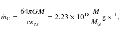
Here the critical accretion rate
 |
(2) |
corresponds to the Eddington luminosity of an accretion disk for a non-rotating BH.
Disk shapes, i.e. the functions z = H(r) describing the vertical half-thickness, are presented in Fig. 1. For the lowest mass accretion rate (
![]() ), the H/r ratio for large radii is about 0.01 while for
), the H/r ratio for large radii is about 0.01 while for
![]() it reaches 0.13. Thus, for the accretion rates considered here, disks are always geometrically very thin,
it reaches 0.13. Thus, for the accretion rates considered here, disks are always geometrically very thin,
For larger accretion rates, the slim disk thickness could be considerably higher. The models calculated by Sadowski (2009) provide the local flux of radiation F(r) in the frame of an observer comoving with the disk. In calculating the continuum spectrum, the standard assumptions have been adopted: (i) radiation from the effective photosphere is locally described by a modified black-body with hardening factor f=1.7 (Shimura & Takahara 1995); (ii) the flux is limb-darkened by
| |
Figure 1:
Disk thickness obtained using a slim disk model for a non-rotating BH. Solutions for three mass accretion rates are presented:
|
| Open with DEXTER | |
For the three accretion rates (1), we calculate the disk spectrum twice: assuming that the effective photosphere coincides with the actual disk surface z = H(r), or that it coincides with the equatorial plane z=0, as if the disk were infinitesimally thin. This means that in the first case we start ray-tracing from z = H(r), and in the second case from z = 0.
![\begin{figure}
\par\includegraphics[width=8.8cm,clip]{11846f2.ps}
\end{figure}](/articles/aa/full_html/2009/28/aa11846-09/img38.png) |
Figure 2:
Emerging continuum spectra of accretion disks calculated for
|
| Open with DEXTER | |
The resulting continuum spectra are plotted in Fig. 2. There are obvious differences between the spectra calculated with the two different assumptions about the location of the effective photosphere, i.e. with the photosphere either at z = H(r), or at z = 0. Even for the moderate mass accretion rate
![]() ,
the ``z = 0'' spectral flux differs from the ``z = H(r)'' flux by about
,
the ``z = 0'' spectral flux differs from the ``z = H(r)'' flux by about ![]() at
at
![]() ,
and for higher accretion rates the
difference is much higher. Such differences should certainly be considered as highly significant.
,
and for higher accretion rates the
difference is much higher. Such differences should certainly be considered as highly significant.
Thus, our result demonstrates that knowing the precise location of the effective photosphere is necessary in calculating the BH slim disk continuum spectra. The effective photosphere lies somewhere between the z = H(r) and z = 0 surfaces.
In principle, the photosphere location could strongly depend on details of the vertical dissipation which are still not sufficiently well known and are therefore assumed ad hoc. This would be bad news. In the rest of this paper we argue that such a situation is unlikely.
Using a simple model for the vertical structure of a geometrically thin, optically thick accretion disk, we show that the photosphere location is not highly sensitive to dissipation. Note that for very thin stationary disks the same is true for the total flux F(r) emitted from a particular radial location - it does not depend on dissipation processes (Shakura & Sunyaev 1973).
These results strengthen one's confidence in estimating the black hole spin by fitting the observed continuum emission of black hole sources to those calculated theoretically (see e.g. Gou et al. 2009; Middleton et al. 2006; Shafee et al. 2006). However, they also indicate that the fitting procedures should be improved to include ray-tracing from the actual location of the photosphere.
3 A simple model of the vertical structure
Our simple model assumes that the accretion disk is geometrically thin (Eq. (3)) and that one may consider radial and vertical disk structure separately.
3.1 Radial equations
We do not solve radial equations, assuming instead that the rotation is strictly Keplerian (in the Kerr geometry),
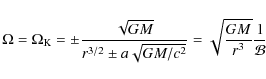
and that the flux F(r) follows from the mass, energy and angular momentum conservation (i.e. does not depend on radial dissipation) and is given by the standard formula (Novikov & Thorne 1973; Page & Thorne 1974),
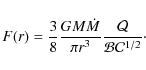
Here M is the black hole mass, a is its specific angular momentum, and
3.2 Vertical equations
We describe the vertical structure of the BH accretion disk in the optically thick regime by the following equations:
- (i)
- The hydrostatic equilibrium:

(6)
where P is the sum of the gas and radiation pressures:
and is the vertical component of the gravitational force of the central object calculated using the relativistic correction factor:
- (ii)
- The energy generation equation:
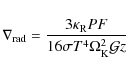
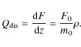
where F is the flux of energy generated inside the disk at a rate given by - the dissipation rate which will be discussed in Sect. 5.1.
- (iii)
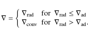
- The generated flux of energy is transported outward through diffusion of radiation and/or convection according to the following thermodynamical relation:
where is the thermodynamical gradient which can be either radiative or convective:
The radiative gradient is calculated using diffusive approximation:
where is the mean Rosseland opacity (see Sect. 3.3) and
  is the Stefan-Boltzmann radiation constant.
- (iv)
- When the temperature gradient is steep enough to exceed the value of the adiabatic gradient
 we have to consider the convective energy flux. The convective gradient
 is calculated using the mixing length theory introduced by Paczynski (1969). We take the following mixing length:
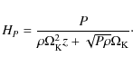
with pressure scale height HP defined as (Hameury et al. 1998):
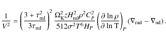
The convective gradient is defined by the following formula:
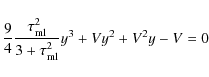
where y is the solution of the equation:
with the typical optical depth for convection and V given by:
The thermodynamical quantities CP,
and
 /
/
 are calculated using standard formulae (e.g. Chandrasekhar 1967) assuming solar abundances (X=0.70, Y=0.28) and taking into account, when necessary, the effect of partial ionization of gas on the gas mean molecular weight.
- (v)
- To close the set of equations describing the vertical structure of an accretion disk, we have to provide boundary conditions. At the equatorial plane (z=0) we put F=0 while at the
disk photosphere we require
 with the flux F given by Page & Thorne (1974).


3.3 Opacities
In this work, we consider optically thick accretion disks. Therefore, we use Rosseland mean opacities
![]() .
The opacities as a function of density and temperature are taken from
Alexander et al. (1983) and Seaton et al. (1994). For temperatures and densities out of both domains we interpolate opacities between these two tables for intermediate values. Following other authors
(e.g. Idan et al. 2008), we neglect expansion opacities, as the vertical velocity gradients in stationary thin disks are expected to be insignificant.
.
The opacities as a function of density and temperature are taken from
Alexander et al. (1983) and Seaton et al. (1994). For temperatures and densities out of both domains we interpolate opacities between these two tables for intermediate values. Following other authors
(e.g. Idan et al. 2008), we neglect expansion opacities, as the vertical velocity gradients in stationary thin disks are expected to be insignificant.
4 Numerical method
The set of ordinary differential equations defined in Sect. 3.2 is solved using the Runge-Kutta method of the 4th order. We start integrating from the equatorial plane (z=0),
where we assume some arbitrary central temperature ![]() ,
density
,
density
![]() and set F=0. We integrate the given set of equations until we reach the photosphere which is defined as a
layer where the following equation is satisfied (corresponding to the optical depth
and set F=0. We integrate the given set of equations until we reach the photosphere which is defined as a
layer where the following equation is satisfied (corresponding to the optical depth ![]() ):
):

5 The photosphere location for a few ad hoc assumed vertical dissipation profiles
We apply our simplified model of vertical structure (Sect. 3) to calculate the photosphere location for different dissipation prescriptions. We test four families of dissipation functions described in the following section.
5.1 Dissipation profiles
First we apply the standard ![]() prescription given by Shakura & Sunyaev (1973). The authors assumed that the source of viscosity in accretion disks is connected with turbulence in gas-dynamical flow, the nature of which was unknown at that time. They based their model on the following expression for the kinematic viscosity coefficient
prescription given by Shakura & Sunyaev (1973). The authors assumed that the source of viscosity in accretion disks is connected with turbulence in gas-dynamical flow, the nature of which was unknown at that time. They based their model on the following expression for the kinematic viscosity coefficient ![]() :
:
(where

and the standard form of the vertical equilibrium:
one can limit the
Therefore, Shakura & Sunyaev (1973) introduced a dimensionless viscosity parameter
This expression for viscosity is called the
is expressed as:
In this work, we apply the regular
In the last decade, several authors (e.g. Hubeny et al. 2001; Hui et al. 2005; Sincell & Krolik 1998; Davis et al. 2005)
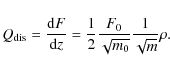
have applied a constant dissipation rate per unit mass. We follow this investigating a class of models using the following formula for the flux generation rate:
Due to the fact that this expression requires not only the total emitted flux F0 but also the total surface density m0, one has to provide the latter based on other disk solutions. In our work, we use models calculated using the regular
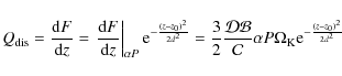
Recent numerical MHD simulations of stratified accretion disks in the shearing box approximation (Davis et al. 2009) show that dissipation rate can be well approximated by the following
formula:
We apply it to another class of models (m-1/2 profile). As in the constant dissipation rate case, we impose surface density profiles obtained using
![\begin{figure}
\par\includegraphics[width=8.8cm,clip]{11846f3.ps}
\end{figure}](/articles/aa/full_html/2009/28/aa11846-09/img98.png) |
Figure 3:
Dissipation profiles for a few representative models at r=20 M. The upper panel presents dissipation functions versus the vertical coordinate z while the bottom panel the former versus surface density
|
| Open with DEXTER | |
Several authors have investigated accretion disks with heat generation concentrated near the equatorial plane or close to the disk surface (e.g. Paczynski & Abramowicz 1982; Paczynski 1980). Therefore, we implement one more class of dissipation prescriptions with an arbitrarily positioned dissipation maximum. We use the following expression
which is the flux generation rate for
where
In Fig. 3 we present dissipation profiles for a few illustrative models. The upper panel presents the flux generation rate versus the vertical coordinate. The ![]() model (solid line)
has a bell-shaped dissipation profile with most of the energy generated at z<0.5 H. The model with a constant dissipation rate per unit mass (thin dashed line) exhibits a very similar behavior.
The dissipation is no longer concentrated around the equatorial plane for the m-1/2 model (thick dashed line) - the maximal flux generation is located at z=0.4 H. However, the dissipation profile is still extended through the whole disk thickness. The arbitrarily positioned models (dot-dashed lines) show the opposite behavior: the energy generation is concentrated around a
given arbitrary location. In the case of the models presented in Fig. 3, the dissipation is confined to altitudes close to the equatorial plane (z=0) and z=0.5 H.
model (solid line)
has a bell-shaped dissipation profile with most of the energy generated at z<0.5 H. The model with a constant dissipation rate per unit mass (thin dashed line) exhibits a very similar behavior.
The dissipation is no longer concentrated around the equatorial plane for the m-1/2 model (thick dashed line) - the maximal flux generation is located at z=0.4 H. However, the dissipation profile is still extended through the whole disk thickness. The arbitrarily positioned models (dot-dashed lines) show the opposite behavior: the energy generation is concentrated around a
given arbitrary location. In the case of the models presented in Fig. 3, the dissipation is confined to altitudes close to the equatorial plane (z=0) and z=0.5 H.
Table 1:
Model assumptions for
![]() .
.
Another point of view on the dissipation profiles is presented in the bottom panel of Fig. 3. The profiles are plotted against the fractional mass surface density m/m0. The right edge of the figure (m=m0) corresponds to the equatorial plane. Two families of models, with dissipation profiles constant and proportional to m-1/2 are represented by straight lines (they are power-law functions of m). As in the upper plot, one can notice a similarity between the ![]() and constant dissipation rate models. The maximum of the flux generation rate for the arbitrarily positioned model centered at z=0.5 H corresponds to the mass depth m=0.1 m0. Obviously, the model centered at the equatorial plane has its maximal dissipation rate at m=m0.
and constant dissipation rate models. The maximum of the flux generation rate for the arbitrarily positioned model centered at z=0.5 H corresponds to the mass depth m=0.1 m0. Obviously, the model centered at the equatorial plane has its maximal dissipation rate at m=m0.
5.2 The photosphere location
We test a number of models representing all four classes of dissipation profiles for a moderate mass accretion rate
![]() .
Details of model parameters are given in Table 1. The location of the disk photospheres is presented in Fig. 4. The first four panels present results for four classes of dissipation profiles in the case of a non rotating BH. A common behaviour is clearly visible: all photosphere locations coincide at radii shorter than 30 M. Outside this radius, the location of the photosphere depends on the assumed dissipation profile and varies between
.
Details of model parameters are given in Table 1. The location of the disk photospheres is presented in Fig. 4. The first four panels present results for four classes of dissipation profiles in the case of a non rotating BH. A common behaviour is clearly visible: all photosphere locations coincide at radii shorter than 30 M. Outside this radius, the location of the photosphere depends on the assumed dissipation profile and varies between
![]() for the
for the ![]() model with the highest value of
model with the highest value of
![]() and
and
![]() for the lowest value
for the lowest value
![]() .
It is of major importance to understand why all photosphere profiles coincide in the inner region, which corresponds to the radiation pressure and electron scattering dominated regime of an accretion disk. The location of the photosphere is defined by Eq. (18). Wherever the radiation pressure and electron scattering dominate in a disk, the left hand side of that formula depends only on the temperature, which is connected at the photosphere to the outgoing flux as
.
It is of major importance to understand why all photosphere profiles coincide in the inner region, which corresponds to the radiation pressure and electron scattering dominated regime of an accretion disk. The location of the photosphere is defined by Eq. (18). Wherever the radiation pressure and electron scattering dominate in a disk, the left hand side of that formula depends only on the temperature, which is connected at the photosphere to the outgoing flux as
![]() .
Therefore, the formula for the energy flux (Eq. (5)) uniquely determines the location of the photosphere in the inner region of a disk independently of the assumed dissipation function. Under these assumptions, we get from Eq. (18):
.
Therefore, the formula for the energy flux (Eq. (5)) uniquely determines the location of the photosphere in the inner region of a disk independently of the assumed dissipation function. Under these assumptions, we get from Eq. (18):

which describes perfectly the photosphere profiles presented in Fig. 4 for r<30 M.
The disk thickness profiles for the case of a rotating BH for three ![]() models are presented in the bottommost panel. They exhibit very similar behaviour: the photosphere location does not
depend on the viscosity prescription for small radii corresponding to the radiation pressure and electron scattering dominated region which, in the case of a rotating BH with a*=0.9, extends inside r=40 M. Therefore, we may infer that such behaviour is general in accretion disks that exhibit radiation pressure dominated regimes. This statement is of paramount importance due to the fact that most of the emission from an accretion disk takes place (in the non-rotating case) between 6 and 20 M. As we have proven, for such radii the photosphere location should not depend on an assumed dissipation profile and, therefore, the spectrum is also likely to be independent of dissipation profile. However, one cannot make sure of this without performing full ray-tracing, which would correctly account for flux emitted from dissipation dependent regions.
The results of this procedure will be discussed in the following section.
models are presented in the bottommost panel. They exhibit very similar behaviour: the photosphere location does not
depend on the viscosity prescription for small radii corresponding to the radiation pressure and electron scattering dominated region which, in the case of a rotating BH with a*=0.9, extends inside r=40 M. Therefore, we may infer that such behaviour is general in accretion disks that exhibit radiation pressure dominated regimes. This statement is of paramount importance due to the fact that most of the emission from an accretion disk takes place (in the non-rotating case) between 6 and 20 M. As we have proven, for such radii the photosphere location should not depend on an assumed dissipation profile and, therefore, the spectrum is also likely to be independent of dissipation profile. However, one cannot make sure of this without performing full ray-tracing, which would correctly account for flux emitted from dissipation dependent regions.
The results of this procedure will be discussed in the following section.
![\begin{figure}
\par\includegraphics[width=8.8cm,clip]{11846f4.ps}
\end{figure}](/articles/aa/full_html/2009/28/aa11846-09/img109.png) |
Figure 4:
Photosphere profiles for different model families for
|
| Open with DEXTER | |
As Shakura & Sunyaev (1973) have shown, for the lowest mass accretion rates the gas dominated region of an accretion disk may extend all the way to the inner edge of a disk. For such a case, the
behavior described in the previous paragraph is not expected: the photosphere profile should depend on the dissipation function at all radii. To account for this fact, we compare photosphere
profiles of accretion disks with low mass accretion rates (Fig. 5). For
![]() the radiation dominated region extends up to
the radiation dominated region extends up to
![]() .
For a lower accretion rate (
.
For a lower accretion rate (
![]() )
it is confined to r<20 M, while for the lowest (
)
it is confined to r<20 M, while for the lowest (
![]() )
it never appears. In that case, the photosphere location indeed depends on the assumed viscosity prescription even for radii shorter than 20 M where most of the
emission comes out. However, one has to bear in mind that the H/r ratio for such low mass accretion rates is even below 0.015 and the impact of the photosphere location on the emerging spectrum should be insubstantial. This is studied in detail in the following section.
)
it never appears. In that case, the photosphere location indeed depends on the assumed viscosity prescription even for radii shorter than 20 M where most of the
emission comes out. However, one has to bear in mind that the H/r ratio for such low mass accretion rates is even below 0.015 and the impact of the photosphere location on the emerging spectrum should be insubstantial. This is studied in detail in the following section.
| |
Figure 5:
Photosphere profiles for |
| Open with DEXTER | |
![\begin{figure}
\par\includegraphics[width=8.5cm,clip]{11846f6.ps}
\end{figure}](/articles/aa/full_html/2009/28/aa11846-09/img116.png) |
Figure 6:
Emerging continuum spectra calculated for different models. The
upper panel presents the number of photons per energy unit crossing a unit surface every second assuming
|
| Open with DEXTER | |
![\begin{figure}
\par\includegraphics[width=8.5cm,clip]{11846f7.ps}
\end{figure}](/articles/aa/full_html/2009/28/aa11846-09/img117.png) |
Figure 7:
Ratios of spectral profiles (photosphere to equatorial)
for models with low mass accretion rates for the perpendicular ( |
| Open with DEXTER | |
5.3 Continuum spectra
To assess the importance of different vertical dissipation profiles on emerging continuum spectra we calculate the latter based on photosphere profiles obtained using our model. For comparison, we
also examine spectra calculated assuming emission from the equatorial plane. Spectra for models with mass accretion rate
![]() are presented in Fig. 6. The upper panel presents total continuum spectra for non- and rapidly-rotating BHs. The spectral profile for the a*=0.9 case extends to higher energies due to the fact that the accretion disk inner edge moves closer to the central object with increasing BH angular momentum, extracting more energetic photons. Spectra for all the photosphere profiles almost coincide and differ significantly from those calculated assuming emission from the equatorial plane. This is clearly visible in the lower panel where we plot the ratio of spectral flux emitted from the photosphere to that emitted from the equatorial plane for the two most extreme photosphere profiles (compare Fig. 4) for each value of BH angular momentum. The spectral profiles are almost identical at energies between
are presented in Fig. 6. The upper panel presents total continuum spectra for non- and rapidly-rotating BHs. The spectral profile for the a*=0.9 case extends to higher energies due to the fact that the accretion disk inner edge moves closer to the central object with increasing BH angular momentum, extracting more energetic photons. Spectra for all the photosphere profiles almost coincide and differ significantly from those calculated assuming emission from the equatorial plane. This is clearly visible in the lower panel where we plot the ratio of spectral flux emitted from the photosphere to that emitted from the equatorial plane for the two most extreme photosphere profiles (compare Fig. 4) for each value of BH angular momentum. The spectral profiles are almost identical at energies between
![]() .
One may conclude that for accretion disks with sufficiently high accretion rate to form the inner radiation pressure supported region, the spectra depend only insignificantly on the vertical dissipation profile in the most interesting range of energies (
.
One may conclude that for accretion disks with sufficiently high accretion rate to form the inner radiation pressure supported region, the spectra depend only insignificantly on the vertical dissipation profile in the most interesting range of energies (
![]() ;
Gou et al. 2009). As was discussed in Sect. 5.2 for the lowest mass
accretion rates (
;
Gou et al. 2009). As was discussed in Sect. 5.2 for the lowest mass
accretion rates (
![]() ), the inner, radiation pressure dominated disk region never appears and the photosphere location depends on the dissipation profile down to the disk inner edge. As it has been pointed out, such a regime of accretion rates implies small values of the H/R ratio. To assess the impact of the dissipation profiles on the continuum spectra, we plotted ratios of corresponding spectral profiles for low and very low mass accretion rates (Fig. 7). The upper panel presents the ratios as observed by an observer perpendicular to the disk plane. The ratios approach 1 with decreasing mass accretion rate. The convergence is very slow due to the fact that the disk thickness in the disk outer region (gas pressure and free-free scatering dominated) depends weakly on the mass accretion rate (
), the inner, radiation pressure dominated disk region never appears and the photosphere location depends on the dissipation profile down to the disk inner edge. As it has been pointed out, such a regime of accretion rates implies small values of the H/R ratio. To assess the impact of the dissipation profiles on the continuum spectra, we plotted ratios of corresponding spectral profiles for low and very low mass accretion rates (Fig. 7). The upper panel presents the ratios as observed by an observer perpendicular to the disk plane. The ratios approach 1 with decreasing mass accretion rate. The convergence is very slow due to the fact that the disk thickness in the disk outer region (gas pressure and free-free scatering dominated) depends weakly on the mass accretion rate (
![]() ,
Shakura & Sunyaev 1973). The difference in spectral flux between models with
,
Shakura & Sunyaev 1973). The difference in spectral flux between models with
![]() and
and
![]() is no greater than
is no greater than ![]() at
at
![]() .
For
an inclined observer (the bottom panel), the departures from the equatorial plane model are much more significant (up to
.
For
an inclined observer (the bottom panel), the departures from the equatorial plane model are much more significant (up to ![]() at
at
![]() ). However, the difference between the spectral fluxes for the models with the two lowest mass accretion rates (corresponding to H/R=0.007 and 0.015, respectively) is still of the order of
). However, the difference between the spectral fluxes for the models with the two lowest mass accretion rates (corresponding to H/R=0.007 and 0.015, respectively) is still of the order of ![]() or even smaller. We conclude that in the lowest accretion rate regime, changes of the photosphere location caused either by different mass accretion rates or different dissipation profiles are insignificant. However, one has to keep in mind that even for mass accretion rates as low as
or even smaller. We conclude that in the lowest accretion rate regime, changes of the photosphere location caused either by different mass accretion rates or different dissipation profiles are insignificant. However, one has to keep in mind that even for mass accretion rates as low as
![]() ,
taking into account the non-zero photosphere location is important for inclined observers as the spectral flux at high energies approaches the equatorial plane limit very slowly.
,
taking into account the non-zero photosphere location is important for inclined observers as the spectral flux at high energies approaches the equatorial plane limit very slowly.
6 Discussion
The results presented here are very encouraging in the context of fitting the calculated optically thick continuum spectra of slim accretion BH disk to the observed continuum emission. Our results imply that the major uncertainties of the accretion disk models, in particular the vertical dissipation profiles, have a rather small influence on the calculated continuum spectra of steady disks with low accretion rates. This is good news for those who use spectral fitting to estimate the spin of black holes.
One should have in mind, however, that there are several effects that have not been taken into account in our simple model, and more theoretical work is needed before fully believable methods of calculating slim disk continuum spectra will be at hand. One of the most obvious (and also quite challenging) theoretical developments needed is a self-consistent and simultaneous solution of the vertical and radial structures of slim, optically thick black hole accretion disks. We are currently working on this problem.
Acknowledgements
This work was initiated at the workshop ``Turbulence and Oscillations in Accretion Discs'' held 1-15 October 2008 at Nordita in Stockholm. We acknowledge Nordita's support. We thank Omer Blaes for his invaluable support and helpful comments. We also acknowledge support from Polish Ministry of Science grants N203 0093/1466, N203 38/436 and 3040/B/H03/2008/35, Swedish Research Council grant VR Dnr 621-2006-3288 and Czech Academy of Sciences grant GAAV 300030510.
References
- Abramowicz, M. A., Czerny, B., Lasota, J. P., & Szuszkiewicz, E. 1988, ApJ, 332, 646 [NASA ADS] [CrossRef]
- Alexander, D. R., Rypma, R. L., & Johnson, H. R. 1983, ApJ, 272, 773 [NASA ADS] [CrossRef] (In the text)
- Bursa, M. 2006, Ph.D. Thesis, Charles University, Prague (In the text)
- Chandrasekhar, S. 1967, An introduction to the study of stellar structure (New York: Dover) (In the text)
- Davis, S. W., Blaes, O., Hubeny, I., & Turner, N. J. 2005, ApJ, 621, 372 [NASA ADS] [CrossRef]
- Davis, S. W., Blaes, O., Hirose, S., & Krolik, J. H. 2009, ApJ, in preparation (In the text)
- Gou, L., McClintock, J. E., Liu, J., et al. 2009, arXiv e-prints
- Hameury, J.-M., Menou, K., Dubus, G., Lasota, J.-P., & Hure, J.-M. 1998, MNRAS, 298, 1048 [NASA ADS] [CrossRef] (In the text)
- Hawley, J. F., & Krolik, J. H. 2002, ApJ, 566, 164 [NASA ADS] [CrossRef] (In the text)
- Hubeny, I., Blaes, O., Krolik, J. H., & Agol, E. 2001, ApJ, 559, 680 [NASA ADS] [CrossRef]
- Hui, Y., Krolik, J. H., & Hubeny, I. 2005, ApJ, 625, 913 [NASA ADS] [CrossRef]
- Idan, I., Lasota, J.-P., Hameury, J.-M., & Shaviv, G. 2008, arXiv e-prints
- Middleton, M., Done, C., Gierlinski, M., & Davis, S. W. 2006, MNRAS, 373, 1004 [NASA ADS] [CrossRef]
- Novikov, I. D., & Thorne, K. S. 1973, in Black Holes, Les Astres Occlus, 343
- Paczynski, B. 1969, Acta Astron., 19, 1 [NASA ADS] (In the text)
- Paczynski, B. 1980, Acta Astron., 30, 347 [NASA ADS]
- Paczynski, B., & Abramowicz, M. A. 1982, ApJ, 253, 897 [NASA ADS] [CrossRef]
- Page, D. N., & Thorne, K. S. 1974, ApJ, 191, 499 [NASA ADS] [CrossRef]
- Rózanska, A., & Madej, J. 2008, MNRAS, 386, 1872 [NASA ADS] [CrossRef]
- Seaton, M. J., Yan, Y., Mihalas, D., & Pradhan, A. K. 1994, MNRAS, 266, 805 [NASA ADS] (In the text)
- Shafee, R., McClintock, J. E., Narayan, R., et al. 2006, ApJ, 636, L113 [NASA ADS] [CrossRef]
- Shakura, N. I., & Sunyaev, R. A. 1973, A&A, 24, 337 [NASA ADS] (In the text)
- Shimura, T., & Takahara, F. 1995, ApJ, 445, 780 [NASA ADS] [CrossRef] (In the text)
- Sincell, M. W., & Krolik, J. H. 1998, ApJ, 496, 737 [NASA ADS] [CrossRef]
- Sadowski, A. 2009, ApJ, accepted (In the text)
- Turner, N. J. 2004, ApJ, 605, L45 [NASA ADS] [CrossRef] (In the text)
Footnotes
- ... disk
![[*]](/icons/foot_motif.png)
- Slim disk is a transsonic solution of an optically thick accretion disk described by vertically integrated equations with simplified (limited to vertical force balance at the surface) treatment of its vertical structure (Abramowicz et al. 1988).
- ...
- This definition is very rough. In the parts of accretion disks that are scattering-dominated, the LTE assumption is not valid and the location of the photosphere is poorly defined.
All Tables
Table 1:
Model assumptions for
![]() .
.
All Figures
| |
Figure 1:
Disk thickness obtained using a slim disk model for a non-rotating BH. Solutions for three mass accretion rates are presented:
|
| Open with DEXTER | |
| In the text | |
| |
Figure 2:
Emerging continuum spectra of accretion disks calculated for
|
| Open with DEXTER | |
| In the text | |
| |
Figure 3:
Dissipation profiles for a few representative models at r=20 M. The upper panel presents dissipation functions versus the vertical coordinate z while the bottom panel the former versus surface density
|
| Open with DEXTER | |
| In the text | |
| |
Figure 4:
Photosphere profiles for different model families for
|
| Open with DEXTER | |
| In the text | |
| |
Figure 5:
Photosphere profiles for |
| Open with DEXTER | |
| In the text | |
| |
Figure 6:
Emerging continuum spectra calculated for different models. The
upper panel presents the number of photons per energy unit crossing a unit surface every second assuming
|
| Open with DEXTER | |
| In the text | |
| |
Figure 7:
Ratios of spectral profiles (photosphere to equatorial)
for models with low mass accretion rates for the perpendicular ( |
| Open with DEXTER | |
| In the text | |
Copyright ESO 2009
Current usage metrics show cumulative count of Article Views (full-text article views including HTML views, PDF and ePub downloads, according to the available data) and Abstracts Views on Vision4Press platform.
Data correspond to usage on the plateform after 2015. The current usage metrics is available 48-96 hours after online publication and is updated daily on week days.
Initial download of the metrics may take a while.