| Issue |
A&A
Volume 501, Number 3, July III 2009
|
|
|---|---|---|
| Page(s) | 1259 - 1268 | |
| Section | Numerical methods and codes | |
| DOI | https://doi.org/10.1051/0004-6361/200911740 | |
| Published online | 29 April 2009 | |
A simple algorithm for optimization and model fitting: AGA (asexual genetic algorithm)
J. Cantó - S. Curiel - E. Martínez-Gómez
Instituto de Astronomía, Universidad Nacional Autónoma de México, Apdo. Postal 70-264, Ciudad Universitaria, Coyoacán, 04510, Mexico
Received 28 January 2009 / Accepted 13 March 2009
Abstract
Context. Mathematical optimization can be used as a computational tool to obtain the optimal solution to a given problem in a systematic and efficient way. For example, in twice-differentiable functions and problems with no constraints, the optimization consists of finding the points where the gradient of the objective function is zero and using the Hessian matrix to classify the type of each point. Sometimes, however it is impossible to compute these derivatives and other type of techniques must be employed such as the steepest descent/ascent method and more sophisticated methods such as those based on the evolutionary algorithms.
Aims. We present a simple algorithm based on the idea of genetic algorithms (GA) for optimization. We refer to this algorithm as AGA (asexual genetic algorithm) and apply it to two kinds of problems: the maximization of a function where classical methods fail and model fitting in astronomy. For the latter case, we minimize the chi-square function to estimate the parameters in two examples: the orbits of exoplanets by taking a set of radial velocity data, and the spectral energy distribution (SED) observed towards a YSO (Young Stellar Object).
Methods. The algorithm AGA may also be called genetic, although it differs from standard genetic algorithms in two main aspects: a) the initial population is not encoded; and b) the new generations are constructed by asexual reproduction.
Results. Applying our algorithm in optimizing some complicated functions, we find the global maxima within a few iterations. For model fitting to the orbits of exoplanets and the SED of a YSO, we estimate the parameters and their associated errors.
Key words: methods: numerical - stars: individual: 55 Cancri - planets and satellites: general - ISM: individual objects: L1448
1 Introduction
Mathematical optimization can be used as a computational tool in deriving the optimal solution for a given problem in a systematic and efficient way. The need to search for parameters that cause a function to be extremal occurs in many kinds of optimization. The optimization techniques fall in two groups: deterministic (Horst & Tuy 1990) and stochastic (Guus et al. 1995). In the first group, we have the classical methods that are useful in finding the optimum solution or unconstrained maxima or minima of continuous and twice-differentiable functions. In this case, the optimization consists of identifying points where the gradient of the objective function is zero and using the Hessian matrix to classify the type of each point. For instance, if the Hessian matrix is positive definite, the point is a local minimum, if it is negative, the point is a local maximum, and if if indefinite, the point is some kind of saddle point. However, the classical methods have limited scope in practical applications since some involve objective functions that are not continuous and/or not differentiable. For these reasons, it is necessary to develop more advanced techniques that belong to the second group. Stochastic models rely on probabilistic approaches and have only weak theoretical guarantees of convergence to the global solution. Some of the most useful stochastic optimization techniques include: adaptive random search (Brooks 1958), clustering methods (Törn 1973), evolutionary computation that includes genetic algorithms, evolutionary strategies and evolutionary programming (Fogel et al. 1966; Schwefel 1995; Goldberg 1989; McCall 2005), simulated and quantum annealing (Kirkpatrick et al. 1983), and neural networks (Bounds 1987).
We present a simple algorithm for optimization (finding the values of the variables that maximize a function) and model fitting (finding the values of the model parameters that fit a set of data most closely). The algorithm may be called genetic, although it differs from standard genetic algorithms (Holland 1975) in the way that new generations are constructed. Standard genetic algorithms involve sexual reproduction, that is, the reproduction by the union of male and female reproductive individuals. Instead, our algorithm uses asexual reproduction, in which offspring are produced by a single parent (as in the fission of bacterial cells).
The paper is organized as follows. In Sect. 2, we present and describe the main characteristics of our algorithm called AGA (asexual genetic algorithm). In Sect. 3, we apply the algorithm to two kinds of problems: maximization of complicated mathematical functions and a model fitting procedure. In the latter group, we consider two examples taken from astronomy: a) the orbital fitting of exoplanets; and b) the model fitting of the Spectral Energy Distribution (SED) observed in a Young Stellar Object (YSO). In both cases, we minimize their corresponding chi-square function. In Sect. 4, we summarize and discuss the results for each case.
2 Description of the AGA (asexual genetic algorithm)
We consider the problem of finding the absolute maxima of a real function of N variables i.e., identifying the values of the N variables (the coordinates of a point in the space of N dimensions) for which the function attains its maximum value. It is assumed that the absolute maximum is inside a bounded region V where the function is defined.
Our algorithm proceeds in the following way (see also Fig. 1):
- 1.
- Construct a random initial population. The initial population is a set of N0 randomly generated points (in the context of evolutionary algorithms, they are also called individuals) within the region V.
- 2.
- Calculate the fitness of each individual in the population. The fitness
is calculated by evaluating the function at each point.
- 3.
- Select a subset of individuals with the highest fitness. Rank the points according to the value of the function, and choose a subset of N1 points with the highest values of the function.
- 4.
- Construct a new population using the individuals in the subset. Generate N2 random points within a previously selected vicinity E around each of the selected points.
- 5.
- Replace the source population with the new population. The new population is the set of
 points that results from step 4 plus a clone of each parent. We may choose (as we did) N1 and N2 such that
 ,
keeping the size of the population N0 unchanged for each generation.
In this way, one can devise an iterative procedure.
,
keeping the size of the population N0 unchanged for each generation.
In this way, one can devise an iterative procedure.
- 6.
- If the stopping criteria (accuracy, maximum number of generations, etc.) have not been met, return to step 2.
![\begin{figure}
\par\includegraphics[width=5.5cm,clip]{1740fig1.eps}
\end{figure}](/articles/aa/full_html/2009/27/aa11740-09/img15.png) |
Figure 1: Basic diagram for the implementation of the asexual genetic algorithm (AGA). First we generate a random initial population. Then, we evaluate the fitness of each individual in this population and select those which have the highest fitness. A new generation is constructed by an asexual reproduction (see text) which replaces the older one. If the stopping criteria are met, we stop. If not, we use these individuals as an initial population and start again. |
| Open with DEXTER | |
For the vicinity E of each selected point, we used rectangular (hyper)boxes of decreasing size. The box around each point was centered on the point and had a side length
![]() along direction i in the generation j. In particular, we take,
along direction i in the generation j. In particular, we take,

where
Decreasing the size of the vicinity E each generation is intended to achieve the highest possible accuracy for the position of the point at which the function attains its absolute maxima. The speed with which the AGA finds a solution depends, of course, on the factor p; the lower the value of p, the faster the solution found. However, if p is too low, the sampling area around the points may decrease so fast that the AGA has no time to migrate to the true solution. On the other hand, if p is too high, many of the offspring will never reach the solution within the convergency criterion. As a consequence of this, the error in the solution will be high and in some cases, the solution will not be reached. The adequate value for p depends on the problem itself. The optimization of p can be achieved by trial and error. However, we have found that a value between 0.4 and 0.6 is adequate for all the tested problems.
An alternative way of choosing the box size consists of employing the standard deviation of the points contained in the subset N1 along each dimension. In such a case, the length of the sides of the box naturally decreases as the algorithm converges. This method works quite efficiently for problems with a few dimensions. Interestingly, the length of the box size in this case decreases following a power law such as that in Eq. (1), with a moderately high values of p (between 0.5-0.8) for the first few generations, abruptly changing to a much lower values (0.2-0.3) for the rest of the generations.
In the case of problems with the large number of parameters to be estimated, we added an iterative method to the scheme presented above. This iterative method consisted of performing a series of runs (each one following the scheme shown in Fig. 1) in such a way that the resultant parameters of a run are taken as the initial ``guess'' for the next run. This procedure may be equivalent to performing a single run allowing for additional generations, but this is not the
case. The key difference is that for each run in the iterative procedure, the sizes of the sampling boxes are reset to their initial values, i.e., each run starts searching for solution using boxes of the same size as those used in the first run but centered on improved initial values. We consider to have reached the optimal solution when the values of the parameters do not change considerably (within a tolerance limit) after several iterations, and the ![]() is found to have
reached a limiting value (see Sect. 3.2.1 and Fig. 7 for an example).
is found to have
reached a limiting value (see Sect. 3.2.1 and Fig. 7 for an example).
We find that this iterative strategy guarantees the convergence to the optimal solution, since it avoids the potential danger of using values of p that do not allow the AGA to drift (migrate) to the ``true'' solution within a single run. Problems that involve the finding of a large number of parameters are potentially subject to this risk, since each parameter may require a different value of p. Furthermore, problems with a large number of parameters become particularly difficult when the values of the different parameters differ by several orders of magnitude, as in the fitting of the orbits of exoplanets and the fitting of the SED of YSOs (see Examples 1 and 2 in Sect. 3). In this case, the iterative method has proven to be particularly useful; the solution usually improves considerably after several iterations.
In the following section, we describe some applications of AGA. We have divided the applications into two groups depending on the type of problem to solve: the maximization of complicated functions and model fitting in astronomy.
3 Applications of the AGA
We separate the optimization problems in two groups. In the first group, we consider functions of two variables where many classical optimization methods present formidable difficulties in finding the global maximum. In the second group, we show two typical examples of model fitting in astronomy that can be treated as minimization procedures.
3.1 Optimization of functions of two variables
There are many examples of functions that are not easy to optimize with classical techniques such as the simplex method, the gradient (or Newton-Raphson) method, the steepest ascent method (Everitt 1987), among others. In such cases, the existence of many maxima (or minima) and the sharpness of the peaks can represent a serious problem. Because of this, the standard Genetic Algorithms or GA are successfully applied in searching for the optimal solution. We consider some typical examples treated by this technique, which are shown below.
3.1.1 Example 1
We consider the following function (Charbonneau 1995):
![\begin{displaymath}%
f\left(x,y\right)=\left[16x\left(1-x\right)y\left(1-y\right)\sin\left(n\pi x\right)\sin\left(n\pi y\right)\right]^{2}
\end{displaymath}](/articles/aa/full_html/2009/27/aa11740-09/img21.png)
where the variables
In Fig. 2, we show the solution to this problem (n=9) by applying AGA after fixing the initial population size, number of parents, number of descendants, and convergency factor (Table 1). Our graphs have the same format as those presented by Charbonneau (1995) to facilitate their comparison.
![\begin{figure}
\par\includegraphics[width=12cm,clip]{1740fig2.ps}
\end{figure}](/articles/aa/full_html/2009/27/aa11740-09/img25.png) |
Figure 2: A solution to the model optimization problem based on the idea of the asexual genetic algorithm. The first five panels show the elevation contours of constant f (Eq. (3) with n=9) and the population distribution of candidate solutions (each one contains 100 points), starting with the initial random population (in the standard GA it is defined as the ``genotype'') in a) and proceeding on through the 25th generation on e). In the sixth panel, we show the evolution of the fittest ``phenotype'' assuming two sizes of the population, N0=100 and N0=400. |
| Open with DEXTER | |
Table 1: Values of the initial parameters used in AGA for the four examples presented in this work.
In the first panel, we start with a population of N0=100 individuals, i.e., a set formed by 100 random points representing the candidate solutions to the global maximum distributed more or less uniformly in parameter space. After 5 generations (second panel), a clustering at the second, third and fourth maxima is clearly apparent. After 10 generations, the solutions already cluster around the main maxima. At the 25th generation, we have reached the maximum in
![]() with
with
![]() with an accuracy of
with an accuracy of
![]() .
We note that at the 25th generation all the 100 individuals have reached
the maximum with at least this accuracy.
.
We note that at the 25th generation all the 100 individuals have reached
the maximum with at least this accuracy.
In the last panel, we show the evolution in the fittest ``phenotype'' with the number of generations as plotted for two sizes of the population, N0=100 and N0=400; in other words, we measure the deviation in the function value for the maxima points identified in each generation
from the ``true'' maximum, that is,
![]() .
It is evident from Fig. 2 that a larger size of the population causes the maximum to be reached in a lower number of generations.
.
It is evident from Fig. 2 that a larger size of the population causes the maximum to be reached in a lower number of generations.
In Fig. 3, we show the evolution in the global solution using AGA and the results obtained by Charbonneau (1995) using a traditional GA. In the first panel for both works, an initial population of 100 individuals is randomly selected. After 10 generations, all the individuals in our algorithm have clustered around the maxima; in contrast, the GA has started to form some clusters. In the third panel, after 20 generations, AGA has found the global maxima, while
the GA continues to search among clusters for a global solution. In the fourth panel, the convergence to the global solution is shown for both works, our AGA having reached the solution in 25 generations with higher accuracy than the 90 generations employed by the GA. In the fifth panel, we finally can compare the evolution in the fittest phenotype for each generation, calculated to be
![]() .
For AGA, these differences are much smaller than those obtained with the GA method, which indicates that our algorithm is more accurate than GA. However, we note that the solution presented in Charbonneau's work was limited by the number of digits used in the encoding scheme. The GA algorithm can also reach high levels of precision by changing the encoding, but at the cost of slower convergence, which would make the GA algorithm become even more computationally expensive than the AGA. The lower number of generations required by AGA to reach a global solution demonstrates that AGA is more efficient than the GA method.
.
For AGA, these differences are much smaller than those obtained with the GA method, which indicates that our algorithm is more accurate than GA. However, we note that the solution presented in Charbonneau's work was limited by the number of digits used in the encoding scheme. The GA algorithm can also reach high levels of precision by changing the encoding, but at the cost of slower convergence, which would make the GA algorithm become even more computationally expensive than the AGA. The lower number of generations required by AGA to reach a global solution demonstrates that AGA is more efficient than the GA method.
![\begin{figure}
\par\includegraphics[width=16cm,clip]{1740fig3.eps}
\end{figure}](/articles/aa/full_html/2009/27/aa11740-09/img32.png) |
Figure 3:
Comparison of our results with those obtained by Charbonneau (1995). We have maintained the same format and removed the curve of the evolution
of the median-fitness individual in the fifth panel of Charbonneau's work to facilitate direct comparison. In the first panel we start with an initial population of 100 individuals and both algorithms start to search the global maxima. While the GA employs 90 generations to reach the solution, our AGA just requires 25 (fourth panels). The fifth panels show the evolution of the fittest phenotype with the number of generations for AGA ( left) and GA ( right). Note that indeed, AGA reaches an accuracy of
|
| Open with DEXTER | |
3.1.2 Example 2
The following example is proposed as a function test in the PIKAIA's user guide (Charbonneau & Knapp 1995). The problem consists of locating the global maximum of the function:
where a and b are known constants, r is the radial distance given by the expression
![\begin{figure}
\par\includegraphics[width=12cm,clip]{1740fig4.ps}
\end{figure}](/articles/aa/full_html/2009/27/aa11740-09/img40.png) |
Figure 4:
Profile of the bi-dimensional positive cosine function. In the upper
panels, we take a=2, b=3 and
|
| Open with DEXTER | |
3.2 The parameter estimation problem in astronomical models
In the physical sciences, curve or model fitting is essentially an optimization problem. Giving a discrete set of N data points
![]() with associated measurement errors
with associated measurement errors
![]() ,
one seeks the best possible model (in other words, the closest fit) for these data using a specific form of the fitting function,
,
one seeks the best possible model (in other words, the closest fit) for these data using a specific form of the fitting function,
![]() .
This function has, in general, several adjustable parameters, whose values are obtained by minimizing a ``merit function'', which measures the agreement between the data and the model function
.
This function has, in general, several adjustable parameters, whose values are obtained by minimizing a ``merit function'', which measures the agreement between the data and the model function
![]() .
.
We suppose that each data point yi has a measurement error that is independently random and distributed as a normal distribution about the ``true'' model with standard deviation
![]() .
The maximum likelihood estimate of the model parameters
.
The maximum likelihood estimate of the model parameters
![]() is then obtained by minimizing the function,
is then obtained by minimizing the function,
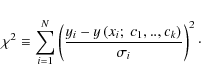
3.2.1 Evaluation of the error estimation
The experimental or observational data are subject to measurement error, thus it is desirable to estimate the parameters in the chosen model and their errors. In the straight-line-data fitting and the general linear least squares,we can compute the standard deviations or variances of individual parameters through simple analytic formulae (Press et al. 1996). However, when we attempt to minimize a function such as Eq. (5), we have no expression for calculating the error in each parameter. A good approach to solve this problem consists of building ``synthetic data sets''. The procedure is to draw random numbers from appropriate distributions so as to mimic our clearest understanding of the underlying process and measurement errors in our apparatus. With these random selections, we compile data sets with exactly the same numbers of measured points and precisely the same values of all control or independent variables, as our true data set. In other words, when the experiment or observation cannot be repeated, we simulate the results we have obtained.
We compiled the synthetic data with the process illustrated in Fig. 5 and from the following expression:
where y'i represents the ith data point of the new set, yi is the ith data point of the original set,
For each of these data sets, we found a corresponding set of parameters (see Fig. 5). Finally, we calculated the average values of each parameter and the corresponding standard deviation, as the estimates of the parameters and their associated errors, respectively. We applied this procedure to the following examples.
Table 2:
Values of the parameters a, b, and
![]() assumed for the function
assumed for the function
![]() and the number of generations needed to reach an error tolerance of 10-6.
and the number of generations needed to reach an error tolerance of 10-6.
| |
Figure 5: From the original set of measurements/observations, several synthetic data sets are constructed. This is achieved by adding to the dependant variable a random number whose absolute value is within the estimated errors of the original data. For each of these synthetic data sets, a set of fitted parameters is obtained. The average value of each parameter and the corresponding standard deviation are taken as estimates of the parameters and their associated errors. |
| Open with DEXTER | |
3.2.2 Fitting the orbits of Extrasolar Giant Planets
We use the merit function given in Eq. (5) and the algorithm described in Sect. 2 to solve an interesting and challenging task in astronomy: curve or model fitting of data for the orbits of the extrasolar planets.
The first extrasolar planet was discovered in 1995 by Mayor & Queloz (1995) and, according to The Extrasolar Planets Encyclopaedia![]() , until February 2009 there had been 342 candidates detected. Most of them (316) were revealed by radial velocity or astrometry of 269 host stars, that is, by Keplerian Doppler shifts in their host stars.
Doppler detectability favors high masses and small orbits depending mainly on the present Doppler errors achievable with available instruments. In addition, the precision of the Doppler technique is probably about 3 m s-1, owing to the intrinsic stability limit of stellar photospheres. This technique is sensitive to companions that induce reflex stellar velocities,
, until February 2009 there had been 342 candidates detected. Most of them (316) were revealed by radial velocity or astrometry of 269 host stars, that is, by Keplerian Doppler shifts in their host stars.
Doppler detectability favors high masses and small orbits depending mainly on the present Doppler errors achievable with available instruments. In addition, the precision of the Doppler technique is probably about 3 m s-1, owing to the intrinsic stability limit of stellar photospheres. This technique is sensitive to companions that induce reflex stellar velocities,
![]() ,
and exhibit orbital periods ranging from a few days to several years, the maximum detectable orbital period being set by the time baseline of the Doppler observations. The remaining exoplanets were detected by other techniques: microlensing (8), imaging (11), and timing (7). For this example we
only refer to the planets detected by radial velocity.
,
and exhibit orbital periods ranging from a few days to several years, the maximum detectable orbital period being set by the time baseline of the Doppler observations. The remaining exoplanets were detected by other techniques: microlensing (8), imaging (11), and timing (7). For this example we
only refer to the planets detected by radial velocity.
![\begin{figure}
\par\includegraphics[width=12cm,clip]{1740fig6.ps}
\end{figure}](/articles/aa/full_html/2009/27/aa11740-09/img52.png) |
Figure 6: The velocities and fits for each of the four planets are shown separately for clarity by subtracting the effects of the other planets. That is, for planet labelled b, planets c, d and e have been removed from the data using the parameters found in the simultaneous four-planet fitting. For planet labelled c we have removed planets b, d and e. For planet labelled d we have removed planets b, c and e. For planet labelled e we have removed planets b, c and d. We have added the fitted systemic velocity for the star, which value is 17.2826 m s-1. The last panel ( bottom and right) shows the residuals between the data and the model. The first (up and left) panel shows the raw data. |
| Open with DEXTER | |
We now consider a system consisting of a central star of mass M*, surrounded by ![]() planets in bounded orbits. Assuming that the orbits are unperturbed Kepler orbits, the line-of-sight velocity of the star relative to the observer (Lee & Peale 2003) is,
planets in bounded orbits. Assuming that the orbits are unperturbed Kepler orbits, the line-of-sight velocity of the star relative to the observer (Lee & Peale 2003) is,
![\begin{displaymath}%
v_{*}=v_{0}+\sum_{j=1}^{N_{p}}K_{j}\left[\cos\left(f_{j}+\omega_{j}\right)+e_{j}\cos~\omega_{j}\right]
\end{displaymath}](/articles/aa/full_html/2009/27/aa11740-09/img54.png)
where ej is the eccentricity,
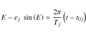
and

where Tj and t0j are the period and time, respectively, of pericenter passage for planet j. Thus, for each planet, there are 5 free parameters: ej, Tj, t0j, Kj and
When these basic parameters for each planet are known through model fitting, we can estimate the semi-major axes of the orbits, aj, and the masses of each planet, mj. To do this, we have to make other simplifying assumptions. For instance, in the simplest model of totally independent planets,
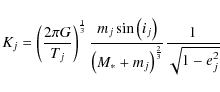
from which we can determine either mj by assuming
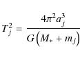
where G denotes the gravitational constant.
We applied the AGA presented in Sect. 2 to the measured radial velocities of the main-sequence star 55 Cancri, published by Fischer et al. (2008).
The data set contains 250 measurements completed at the Lick Observatory from 1989 to 2007, and 70 measurements made at the Keck Observatory from 2002 to 2007 of the velocity of 55 Cancri. Data from Lick has measurement errors of
![]() (1989-1994) and 3-5
(1989-1994) and 3-5
![]() (1995-2007). Data from Keck has measurement errors of 3
(1995-2007). Data from Keck has measurement errors of 3
![]() for data acquired prior to 2004 August and 1.0-1.5
for data acquired prior to 2004 August and 1.0-1.5
![]() thereafter. The measured data have a maximum amplitude of
thereafter. The measured data have a maximum amplitude of
![]() and are of excellent signal-to-noise ratio. The orbital parameters were established by the detection of four planets in all Doppler measurements.
To test a possible stellar systemic velocity remnant in the data, we added an additional parameter to the systemic velocity of the star obtaining a value of 17.28
and are of excellent signal-to-noise ratio. The orbital parameters were established by the detection of four planets in all Doppler measurements.
To test a possible stellar systemic velocity remnant in the data, we added an additional parameter to the systemic velocity of the star obtaining a value of 17.28
![]() .
We fitted the orbits of 1-4 planets to this data (see Fig. 6). This exercise shows that the fitting solution improves when considering the orbit of more planets. The rms of the residuals and the
.
We fitted the orbits of 1-4 planets to this data (see Fig. 6). This exercise shows that the fitting solution improves when considering the orbit of more planets. The rms of the residuals and the
![]() ,
,
![]() values, improve from values of 33.5 and 9.72, respectively, when fitting
the orbit of one planet, to values of 7.99 and 2.03, respectively, when fitting the orbit of four planets (see Table 3). In general, the values of the rms,
values, improve from values of 33.5 and 9.72, respectively, when fitting
the orbit of one planet, to values of 7.99 and 2.03, respectively, when fitting the orbit of four planets (see Table 3). In general, the values of the rms,
![]() fits and the derived parameters compare well with those obtained by Fischer et al. (2008). In Tables 3 and 4, we summarize our results.
fits and the derived parameters compare well with those obtained by Fischer et al. (2008). In Tables 3 and 4, we summarize our results.
Table 3:
Our values of the rms of the residuals and the
![]() fits for the orbital fitting problem using AGA.
fits for the orbital fitting problem using AGA.
With the exceptions of the third and fourth planet fittings, our rms values are lower than those obtained by Fischer et al. (2008). Our
![]() values are however lower in all cases.
values are however lower in all cases.
From the parameters shown in Table 4 we were able to derive the mass of the planet,
![]() (MJ), and the major semiaxis a (AU). For the four-planet fitting, we found (Table 5) that our values compare well with those reported by Fischer et al. (2008) in their five-planet model. Except for the first planet, all the values for the major semiaxis have a standard error lower than those obtained in the Fischer's model. In the case of the mass of each planet, our values have smaller standard errors.
(MJ), and the major semiaxis a (AU). For the four-planet fitting, we found (Table 5) that our values compare well with those reported by Fischer et al. (2008) in their five-planet model. Except for the first planet, all the values for the major semiaxis have a standard error lower than those obtained in the Fischer's model. In the case of the mass of each planet, our values have smaller standard errors.
We included the iterative scheme discussed in Sect. 2 in fitting the orbit of the planets. In Fig. 7, we show the value of the
![]() for the four-planet fit calculated after each run. In this case, we started with
for the four-planet fit calculated after each run. In this case, we started with
![]() and after the 10th iterative run, the
and after the 10th iterative run, the
![]() had diminished to 4.15, which means that we had not found the optimal solution. During the first iterative runs, we note that the value of
had diminished to 4.15, which means that we had not found the optimal solution. During the first iterative runs, we note that the value of
![]() decreased rapidly. After about 100 iterative runs, the
decreased rapidly. After about 100 iterative runs, the
![]() had not changed significally and converged to a fixed value (there are only slight variations in the last decimals). At this point, we can be assured that the value of the parameters have been found. Finally,
we estimated the errors in fitting the orbits of the four planets as described in Sect. 3.2.1. We present the estimated errors in Tables 4 and 5.
had not changed significally and converged to a fixed value (there are only slight variations in the last decimals). At this point, we can be assured that the value of the parameters have been found. Finally,
we estimated the errors in fitting the orbits of the four planets as described in Sect. 3.2.1. We present the estimated errors in Tables 4 and 5.
Table 4: Our estimated values for the five parameters of the four exoplanets around 55 Cancri.
Table 5: Our derived values for the mass of the planet and the major semiaxis for the four-planet fitting.
3.2.3 Fitting the spectral energy distribution (SED) for a YSO
A spectral energy distribution (SED) is a plot of flux, brightness or flux density versus frequency/wavelength of light. It is widely used to characterize astronomical sources i.e., to identify the type of source (star, galaxy, circumstellar disk) that produces these fluxes
or brightness. Modelling the observed SEDs can help us to infer the temperature and size, among the other physical parameters of the source. As examples in radio astronomy, a SED with a negative spectral index
![]() would indicate the presence of a synchrotron radiation source; in infrared astronomy, SEDs can be used to classify T-Tauri stars; in galactic astronomy, the analysis of the SEDs leads to the determination of the respective roles of the old and young stellar
populations in dust-grain heating.
would indicate the presence of a synchrotron radiation source; in infrared astronomy, SEDs can be used to classify T-Tauri stars; in galactic astronomy, the analysis of the SEDs leads to the determination of the respective roles of the old and young stellar
populations in dust-grain heating.
![\begin{figure}
\par\includegraphics[width=8cm,clip]{1740fig7.eps}
\end{figure}](/articles/aa/full_html/2009/27/aa11740-09/img77.png) |
Figure 7:
Convergence of the
|
| Open with DEXTER | |
For the reasons explained above, it is interesting to find the adequate model for an observed SED. We consider the observations reported by Curiel et al. (2009) in the L1448 region. This cloud is part of the Perseus molecular cloud complex located at a distance of
![]() .
We are interested in fitting the observed SED for a couple of reasons: it contains an extremely young and highly collimated bipolar outflow (Bachiller et al. 1990) and seems to be a site of very recent star formation based on some observations (Anglada et al. 1989; Curiel et al. 1990; Barsony et al. 1998; Girart & Acord 2001;
Reipurth et al. 2002).
.
We are interested in fitting the observed SED for a couple of reasons: it contains an extremely young and highly collimated bipolar outflow (Bachiller et al. 1990) and seems to be a site of very recent star formation based on some observations (Anglada et al. 1989; Curiel et al. 1990; Barsony et al. 1998; Girart & Acord 2001;
Reipurth et al. 2002).
The data are taken from Curiel et al. (2009), who carried out a fit of the SED by assuming that there are three main components contributing to the flux at different wavelengths. Thus, the fitting function was given by the contribution of an optically free-free component
and two grey bodies:
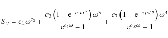
where
The free parameters to be estimated, by the minimization of the chi-square (Eq. (5)), are identified as
c1,c2,...,c10. They are defined in terms of their corresponding physical parameters as:
![]() is the flux of optically thin emission with a spectral index given by
is the flux of optically thin emission with a spectral index given by
![]() ,
which corresponds to the free-free emission coming from a thermal jet;
,
which corresponds to the free-free emission coming from a thermal jet;
![]() is a reference flux;
is a reference flux;
![]() is the dust opacity evaluated at the reference frequency
is the dust opacity evaluated at the reference frequency ![]() ;
;
![]() is the dust emissivity index; and
is the dust emissivity index; and
![]() is related to the temperature. The last four parameters correspond to the emission originating in the first grey body (probably a molecular
envelope). Finally, we propose that a second grey body exists that is a circumstellar disk surrounding the young protostar. Similarly, the parameters c7, c8, c9, and c10 are related to the physical parameters of the second grey body.
is related to the temperature. The last four parameters correspond to the emission originating in the first grey body (probably a molecular
envelope). Finally, we propose that a second grey body exists that is a circumstellar disk surrounding the young protostar. Similarly, the parameters c7, c8, c9, and c10 are related to the physical parameters of the second grey body.
In the previous expressions, ![]() is the frequency at which the source is observed, h is the Planck's constant,
is the frequency at which the source is observed, h is the Planck's constant, ![]() is the solid angle subtended by the source, c is the speed of light,
is the solid angle subtended by the source, c is the speed of light,
![]() is the optical depth at the frequency
is the optical depth at the frequency ![]() for each component,
for each component, ![]() is the dust emissivity index for each component, and k is the Boltzmann's constant. We assumed the characteristic frequency of the source to be
is the dust emissivity index for each component, and k is the Boltzmann's constant. We assumed the characteristic frequency of the source to be
![]() (Curiel
et al. 2009). Table 6 summarizes the values of the fitted parameters in the model described by Eq. (12) of the SED for a YSO in the L1448 region. Table 6 also includes the estimated errors in the fitted parameters, as described in Sect. 3.3.1. Figure 8 shows the observed data together with the best fit.
(Curiel
et al. 2009). Table 6 summarizes the values of the fitted parameters in the model described by Eq. (12) of the SED for a YSO in the L1448 region. Table 6 also includes the estimated errors in the fitted parameters, as described in Sect. 3.3.1. Figure 8 shows the observed data together with the best fit.
Table 6: Estimated values for the ten parameters in the model of the SED for a YSO in the L1448 region.
From Fig. 8, we can conclude that the fitted model with the parameters shown in Table 6 is adequate for explaining the observations of the YSO in the L1448 region. The fitted curve lies within the measurement error bars (except one point located at high frequencies) and the SED consists of a continuum component and the emission from two grey bodies. Further astrophysical implications of these results can be found in Curiel et al. (2009).
4 Summary and conclusions
We have presented a simple algorithm based on the idea of genetic algorithms to optimize functions. Our algorithm differs from standard genetic algorithms mainly in mainly two respects: 1) we do not encode the initial information (that is, the initial set of possible solutions to the optimization problem) into a string of binary numbers and 2) we propose an asexual reproduction as a means of obtaining new ``individuals'' (or candidate solutions) for each generation.
We have then applied the algorithm in solving two types of optimization problems: 1) finding the global maximum in functions of two variables, where the typical techniques fail; and 2) parameter estimation in astronomy by the minimization of the chi-square. For the latter case, we considered two examples: fitting the orbits of extrasolar planets associated with the star 55 Cancri and fitting the SED of a YSO for the L1448 region.
![\begin{figure}
\par\includegraphics[width=8cm,clip]{1740fig8.ps}
\end{figure}](/articles/aa/full_html/2009/27/aa11740-09/img100.png) |
Figure 8: The Spectral Energy Distribution (SED) for a YSO in the L1448 region. The dots represent the observations and the bars their associated measurement errors. The straight line corresponds to the continuum flux, the dashed line is the first grey body, the dotted line is the second grey body and the solid line is the sum of the three contributions. |
| Open with DEXTER | |
We found that our algorithm has several advantages:
- It is easy to implement in any computer because it does not require an encoding/decoding routine, and the new generations are constructed by the asexual reproduction of a selected subset (with the highest fitness) of the previous population.
- The algorithm does not require the evaluation of standard genetic operations such as crossover and mutation. This is replaced by a set of sampling rules, which simplifies the creation of new generations and speeds up the finding of the best solution.
- When the initial ``guess'' is far from the solution, AGA is capable to migrate searching for the ``true'' optimal solution. The final solution is usually achieved after a few hundred generations, in some cases, even faster.
- In some difficult cases, such as the fitting of the orbits of several exoplanets and the fitting of the SED of YSOs (with several components), AGA finds the solution in a few hundred generations. In these cases, an iterative scheme (several runs of AGA using the solutions of one
run as the initial ``guess'' of the next run) can help to improve finding the ``true'' solution. This is particularly useful when the variables have different orders of magnitude, which causes the
different variables to not converge to the final solution at the same time.
- As a consequence of the previous points, AGA becomes computationally less expensive than the standard version (GA). The convergence of AGA is reached in just a few generations.
In the case of the SED for a YSO in the L1448 region, we find that the most adequate model contains the contribution of two grey bodies at high frequencies and free-free continuum emission, through a power law, at low frequencies.
Generally speaking the implementation of any kind of GA is advantageous in the sense that we do not have to compute any derivative of the selected fitness function allowing us to optimize functions with several local maxima points.
In this work, we have also implemented a method to estimate the error associated with each parameter based on the generation of ``synthetic data sets''. This method is easy to implement in any type of measured/observed data and constitutes a way of estimating the errors in the parameters
when the minimization of the ![]() is employed.
is employed.
Acknowledgements
We acknowledge the support of CONACyT (Mexico) grants 61547 and 60581. E.M.G. also thanks to DGAPA-UNAM postdoctoral fellowship for the financial support provided for this research. We thank the anonymous referee for the helpful comments made to this work.
References
- Anglada, G., Rodríguez, L. F., Torrelles, J. M., et al. 1989, ApJ, 341, 208 [NASA ADS] [CrossRef] (In the text)
- Bachiller, R., Martin-Pintado, J., Tafalla, M., Cernicharo, J. & Lazareff, B. 1990, A&A, 231(1), 174 (In the text)
- Barsony, M., Ward-Thompson, D., André, P., & O'Linger, J. 1998, ApJ, 509, 733 [NASA ADS] [CrossRef] (In the text)
- Bounds, D. 1987, Nature, 329, 215 [NASA ADS] [CrossRef] (In the text)
- Brooks, S. H. 1958, Op. Res., 6, 244 [CrossRef] (In the text)
- Charbonneau, P. 1995, ApJS, 101, 309 [NASA ADS] [CrossRef] (In the text)
- Charbonneau, P., & Knapp, B. 1995, A User's guide to PIKAIA 1.0, NCAR Technical Note 418+IA (Boulder: National Center for Atmospheric Research)
- Curiel, S., Raymond, J. C., Moran, J. M., Rodríguez, L. F., & Cantó, J. 1990, ApJ, 365, L85 [NASA ADS] [CrossRef] (In the text)
- Curiel, S., Girart, J. M., Fernández-López, M., Cantó, J., & Rodríguez, L. F. 2009, ApJ, submitted (In the text)
- Everitt, B. S. 1987, in Introduction to optimization methods and their application to statistics (UK: Chapman & Hall, Ltd) (In the text)
- Fischer, D. A., Marcy, G. W., Butler, R. P., et al. 2008, ApJ, 675, 790 [NASA ADS] [CrossRef]
- Fogel, L. J., Owens A. J., & Walsh, M. J. 1966, Artificial Intelligence through simulated evolution (New York: Wiley & Sons) (In the text)
- Girart, J. M., & Acord, J. M. P. 2001, ApJ, 552, L63 [NASA ADS] [CrossRef]
- Goldberg, D. E. 1989, in Genetic Algorithms in Search, Optimization and Machine Learning (USA: Addison Wesley Longman Publishing Co) (In the text)
- Guus, C., Boender, E., & Romeijn, H. E. 1995, Stochastic methods, in Handbook of global optimization, ed. R. Horst, & P. M. Pardalos (Dordrecht, The Netherlands: Kluwer Academic Publishers), 829 (In the text)
- Holland, J. 1975, in Adaptation in Natural and Artificial Systems (In the text)
- Horst, R., & Tuy, H. 1990, in Global optimization: Deterministic approaches (Berlin: Springer-Verlag) (In the text)
- Kirkpatrick, S., Gellatt, C. D., & Vecchi, M. P. 1983, Science, 220, 671 [NASA ADS] [CrossRef] (In the text)
- Lee, M. H., & Peale, S. J. 2003, ApJ, 592, 1201 [NASA ADS] [CrossRef]
- Marcy, G. W., Butler R. P., Fischer, D. A., et al. 2002, ApJ, 581, 1375 [NASA ADS] [CrossRef] (In the text)
- McCall, J. 2005, J. Comput. Appl. Math., 184, 205 [NASA ADS] [CrossRef] (In the text)
- Mayor, M., & Queloz, D. 1995, Nature, 378, 355 [NASA ADS] [CrossRef] (In the text)
- Press, W. H., Teukolsky, S. A., Vetterling, W. T., & Flannery, B. P. 1996, in Numerical recipes in Fortran 77 (UK: Cambridge University Press), 1 (In the text)
- Reipurth, B., Rodríguez, L. F., Anglada, G., & Bally, J. 2002, AJ, 124, 1045 [NASA ADS] [CrossRef] (In the text)
- Schwefel, H. P. 1995, in Evolution and optimum seeking (New York: Wiley & Sons) (In the text)
- Törn, A. 1973, Global optimization as a combination of global and local search, Proceedings of computer simulation versus analytical solutions for business and economic models, Gothenburg, Sweden, 191 (In the text)
Footnotes
All Tables
Table 1: Values of the initial parameters used in AGA for the four examples presented in this work.
Table 2:
Values of the parameters a, b, and
![]() assumed for the function
assumed for the function
![]() and the number of generations needed to reach an error tolerance of 10-6.
and the number of generations needed to reach an error tolerance of 10-6.
Table 3:
Our values of the rms of the residuals and the
![]() fits for the orbital fitting problem using AGA.
fits for the orbital fitting problem using AGA.
Table 4: Our estimated values for the five parameters of the four exoplanets around 55 Cancri.
Table 5: Our derived values for the mass of the planet and the major semiaxis for the four-planet fitting.
Table 6: Estimated values for the ten parameters in the model of the SED for a YSO in the L1448 region.
All Figures
| |
Figure 1: Basic diagram for the implementation of the asexual genetic algorithm (AGA). First we generate a random initial population. Then, we evaluate the fitness of each individual in this population and select those which have the highest fitness. A new generation is constructed by an asexual reproduction (see text) which replaces the older one. If the stopping criteria are met, we stop. If not, we use these individuals as an initial population and start again. |
| Open with DEXTER | |
| In the text | |
| |
Figure 2: A solution to the model optimization problem based on the idea of the asexual genetic algorithm. The first five panels show the elevation contours of constant f (Eq. (3) with n=9) and the population distribution of candidate solutions (each one contains 100 points), starting with the initial random population (in the standard GA it is defined as the ``genotype'') in a) and proceeding on through the 25th generation on e). In the sixth panel, we show the evolution of the fittest ``phenotype'' assuming two sizes of the population, N0=100 and N0=400. |
| Open with DEXTER | |
| In the text | |
| |
Figure 3:
Comparison of our results with those obtained by Charbonneau (1995). We have maintained the same format and removed the curve of the evolution
of the median-fitness individual in the fifth panel of Charbonneau's work to facilitate direct comparison. In the first panel we start with an initial population of 100 individuals and both algorithms start to search the global maxima. While the GA employs 90 generations to reach the solution, our AGA just requires 25 (fourth panels). The fifth panels show the evolution of the fittest phenotype with the number of generations for AGA ( left) and GA ( right). Note that indeed, AGA reaches an accuracy of
|
| Open with DEXTER | |
| In the text | |
| |
Figure 4:
Profile of the bi-dimensional positive cosine function. In the upper
panels, we take a=2, b=3 and
|
| Open with DEXTER | |
| In the text | |
| |
Figure 5: From the original set of measurements/observations, several synthetic data sets are constructed. This is achieved by adding to the dependant variable a random number whose absolute value is within the estimated errors of the original data. For each of these synthetic data sets, a set of fitted parameters is obtained. The average value of each parameter and the corresponding standard deviation are taken as estimates of the parameters and their associated errors. |
| Open with DEXTER | |
| In the text | |
| |
Figure 6: The velocities and fits for each of the four planets are shown separately for clarity by subtracting the effects of the other planets. That is, for planet labelled b, planets c, d and e have been removed from the data using the parameters found in the simultaneous four-planet fitting. For planet labelled c we have removed planets b, d and e. For planet labelled d we have removed planets b, c and e. For planet labelled e we have removed planets b, c and d. We have added the fitted systemic velocity for the star, which value is 17.2826 m s-1. The last panel ( bottom and right) shows the residuals between the data and the model. The first (up and left) panel shows the raw data. |
| Open with DEXTER | |
| In the text | |
| |
Figure 7:
Convergence of the
|
| Open with DEXTER | |
| In the text | |
| |
Figure 8: The Spectral Energy Distribution (SED) for a YSO in the L1448 region. The dots represent the observations and the bars their associated measurement errors. The straight line corresponds to the continuum flux, the dashed line is the first grey body, the dotted line is the second grey body and the solid line is the sum of the three contributions. |
| Open with DEXTER | |
| In the text | |
Copyright ESO 2009
Current usage metrics show cumulative count of Article Views (full-text article views including HTML views, PDF and ePub downloads, according to the available data) and Abstracts Views on Vision4Press platform.
Data correspond to usage on the plateform after 2015. The current usage metrics is available 48-96 hours after online publication and is updated daily on week days.
Initial download of the metrics may take a while.