Swift observations of the very intense flaring activity of Mrk 421 during 2006. I. Phenomenological picture of electron acceleration and predictions for MeV/GeV emission

A. Tramacere; P. Giommi; M. Perri; F. Verrecchia; G. Tosti

doi:10.1051/0004-6361/200810865

Free Access

Issue		A&A Volume 501, Number 3, July III 2009


Page(s)		879 - 898
Section		Extragalactic astronomy
DOI		https://doi.org/10.1051/0004-6361/200810865
Published online		29 April 2009

Swift observations of the very intense flaring activity of Mrk 421 during 2006. I. Phenomenological picture of electron acceleration and predictions for MeV/GeV emission

A. Tramacere^1,2 - P. Giommi³ - M. Perri³ - F. Verrecchia³ - G. Tosti^4,5

1 - CIFS - Torino, Viale Settimio Severo 3, 10133 Torino, Italy
2 - SLAC, 2575 Sand Hill Road, Menlo Park, CA 94025, USA
3 - ASI Science Data Center, c/o ESRIN, via G. Galilei, 00044 Frascati, Italy
4 - Dipartimento di Fisica, via A. Pascoli, 06100 Perugia, Italy
5 - INFN Perugia, via A. Pascoli, 06100 Perugia, Italy

Received 27 August 2008 / Accepted 28 January 2009

Abstract
Aims. We present the results of a deep spectral analysis of all Swift observations of Mrk 421 between April 2006 and July 2006, when it reached its highest X-ray flux recorded until the end of 2006. The peak flux was about 85 milli-Crab in the 2.0-10.0 keV band, and the peak energy ( $E_{\rm p}$ ) of the spectral energy distribution (SED) was often at energies higher than 10 keV. We study trends between the spectral parameters, and the physical insights the parameters provide into the underlying acceleration and emission mechanisms.
Methods. We performed a spectral analysis of Swift observations to investigate trends between the spectral parameters. We searched for acceleration and energetic features phenomenologically linked to the SSC model parameters, by predicting their effects in the $\gamma$ -ray band, and in particular, the spectral shape expected in the Fermi Gamma-ray Space Telescope-LAT band.
Results. We confirm that the X-ray spectrum is described well by a log-parabolic distribution close to $E_{\rm p}$ , that the peak flux of the SED ( $S_{\rm p}$ ) is correlated with $E_{\rm p}$ , and that $E_{\rm p}$ is anti-correlated with the curvature parameter (b). The spectral evolution in the Hardness-ratio-flux plane shows both clockwise and counter-clockwise patterns. During the most energetic flares, the UV-to-soft-X-ray spectral shape requires an electron distribution spectral index of $s\simeq 2.3$ .
Conclusions. We demonstrate that the UV-to-X-ray emission from Mrk 421 is probably generated by a population of electrons that is actually curved, and has a low energy power-law tail. The observed spectral curvature is consistent with both stochastic acceleration or energy-dependent acceleration probability mechanisms, whereas the power-law slope of XRT-UVOT data is close to that inferred from the GRBs X-ray afterglow and in agreement with the universal first-order relativistic shock acceleration models. This scenario implies that magnetic turbulence may play a twofold role: spatial diffusion relevant to the first order process and momentum diffusion relevant to the second order process.

Key words: galaxies: active - galaxies: BL Lacertae objects: individual: Mrk 421- X-rays: individuals: Mrk 421 - radiation mechanisms: non-thermal - acceleration of particles

1 Introduction

BL Lac objects are Active Galactic Nuclei (AGNs) characterized by a polarised and highly variable nonthermal continuum emission extending from radio to $\gamma$ -rays. In the most accepted scenario, this radiation is produced within a relativistic jet that originates in the central engine and points close to our line of sight. The relativistic outflow has a typical bulk Lorentz factor of $\Gamma \approx 10$ , hence the emitted fluxes, observed at an angle $\theta$ , are affected by a beaming factor $\delta = 1/(\Gamma (1 - \beta \cos\theta ))$ .

The Spectral Energy Distribution (SED) of these objects has a typical two-bump shape. According to current models, the lower-frequency bump is interpreted as synchrotron emission from highly relativistic electrons with Lorentz factors $\gamma$ in excess of 10². This component peaks at frequencies ranging from the IR to the X-ray band. The true position of this peak was proposed by Padovani & Giommi (1995) as an indicator in classifying sources; they define LBL (Low energy peaked BL Lac) to be objects with the first bump in the IR-to-optical band, and HBL (High energy peaked BL Lac) as those with SEDs peaking in the UV-X-ray band. According to the Synchrotron Self Compton (SSC) emission mechanism, the higher-frequency bump can be attributed to inverse Compton scattering of synchrotron photons by the same population of relativistic electrons that produce the synchrotron emission (Jones et al. 1974; Ghisellini & Maraschi 1989).

Table 1: Swift observation journal and exposures of Mrk 421.

With its redshift z = 0.031, Mrk 421 is among the closest and most well studied HBL. It is one of brightest BL Lac objects in the UV and the X-ray bands, and was observed in $\gamma$ rays by EGRET (Lin et al. 1992); it was also the first extragalactic source detected at TeV energies in the range 0.5-1.5 TeV by the Whipple telescopes (Petry et al. 1996; Punch et al. 1992).

The source is classified as HBL because its synchrotron emission peak ranges from a fraction of a keV to several keV. Its flux variations go along with significant spectral variations (Massaro et al. 2004; Fossati et al. 2000a) and the spectral shape in general exhibits a curvature that is described well by a log-parabolic model (Massaro et al. 2004; Tramacere et al. 2007b).

In spring/summer 2006, Mrk 421 reached its highest X-ray flux recorded until that time. The peak flux was about 85 milli-Crab in the 2.0-10.0 keV band, and corresponded to a peak energy of the spectral energy distribution (SED) that was often at energies higher than 10 keV.

In this paper (Paper I), we present data collected from Swift observations performed during this intense flaring period. We study the evolution in the spectral parameters as a function of the flaring activity, and the correlations between the spectral parameters. This provides a phenomenological picture of the physical mechanism driving the observed patterns. In Paper II, we will frame this scenario in the theoretical context of stochastic acceleration (Tramacere 2009).

In the phenomenological context of jets in HBLs, the spectral curvature is relevant to the understanding of both the radiative and acceleration mechanisms.

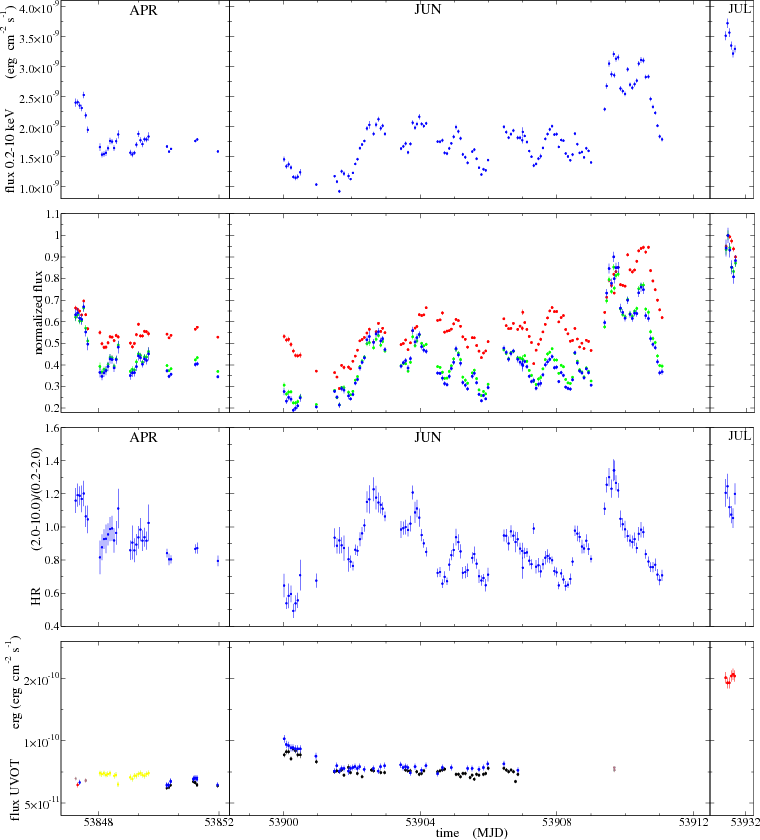$\begin{figure} \par\epsfig{file=0865fig1a.ps,width=3.4cm,angle=-90}\\ \epsfig{f... ....4cm,angle=-90}\\ \epsfig{file=0865fig1d.ps,width=3.4cm,angle=-90} \end{figure}$

Figure 1:

From top to bottom: a) light curve of the flux in the band 0.2-10.0 keV. b) light curves for three different bands soft (0.2-3.0 keV, red points) medium (3.0-5.0 keV, green points) and hard ( 5.0-10.0 keV, blue points), normalized to their maximum value. c) the evolution of the hardness ratio (HR) evaluated as the ratio of the 2.0-10.0 keV band to the 0.2-2.0 keV band. d) light curve from the Swift-UVOT instrument, different colors refers to different filters (V = brown, U = black, UVM2 = red, UVW1 = blue, UVW2 = yellow). (See the electronic edition of the Journal for a color version of this figure)

Open with DEXTER

Many studies have demonstrated that the X-ray spectral shape of Mrk 421 is curved and described by a log-parabolic distribution with a mildly curved and symmetric spectral shape (Tanihata et al. 2004; Massaro et al. 2004; Tramacere et al. 2007a; Fossati et al. 2000b). Massaro et al. (2004) interpreted this feature in the framework of energy-dependent acceleration efficiency that naturally corresponds to log-parabolic spectral distributions with a possible power-law tail at lower energies. Kardashev (1962) showed that a log-parabolic distribution results from a stochastic acceleration scenario with a mono-energetic or quasi-mono energetic particle injection. Katarzynski et al. (2006) and Giebels et al. (2007) used a relativistic Maxwellian electron distribution, produced by a stochastic acceleration process, to describe the X-ray/TeV emission of Mrk 501 and Mrk 421 , respectively. Stawarz & Petrosian (2008) showed that a distribution with similar spectral properties can be obtained as a steady-state energy spectra of particles undergoing momentum diffusion due to resonant interactions with turbulent MHD modes.

Tramacere et al. (2007b) suggested that the connection between the X-ray curvature and the emitting particles, and its evolution with the source state, could be investigated in testing the prediction of the scenarios listed above. In particular, both stochastic (Kardashev 1962) and energy-dependent acceleration mechanisms predict an anticorrelation between the curvature and the SED peak energy ( $E_{\rm p}$ ). The pattern traced by the peak height ( $S_{\rm p}$ ) of the SED as $E_{\rm p}$ varies, can indicate the evolution in the parameters characterizing the energetics of the synchrotron emission, in particular the average particle energy and the number density of the emitting particles.

During the most violent flares, a crucial issue is to understand whether the shape of the X-ray spectrum can also be described by a single log-parabolic spectral distribution. A typical X-ray detector shows only a slice (usually up to two decades in energy) of the overall emission from the observed object. During strong flares involving significant variation in the SED peak energy, it is possible to understand whether the electron distribution is curved even far from the peak energy. We can also benefit from the unique opportunity provided by Swift to perform simultaneous UV-to-X-ray observations, and extend the spectral window from about 10¹⁵ Hz to 10¹⁹ Hz. The presence of a power-law tail at low photon energies and its slope can provide information about the low-energy tail of the underlying electron distribution as well as the acceleration mechanism generating such a spectral shape.

By developing the phenomenological results from the present analysis, we attempt to model the SED of Mrk 421 within the synchrotron-self-Compton (SSC) scenario, predicting the possible spectral behaviour at $\gamma$ -ray energies. In particular, we are able to relate the typical spectral shape of the UV-to-soft-X-ray emission to that expected in the MeV/GeV band covered by the Fermi Gamma-ray Space Telescope-LAT instrument.

This paper is organized as follows. In Sect. 2, we present our data set and the procedure used to reduce the Swift data. In Sect. 3, we report the results of an analysis of the rapid variability of the source. In Sect. 4 we present spectral analysis results. In Sect. 5 we analyse the spectral evolution of the source. In Sect. 6 we study the correlations between the spectral parameters and compare these results with those of previous studies directing particular attention to the link between these trends and expectations from different scenarios for the acceleration mechanism. In Sect. 7, we study the connection between the UVOT and the XRT spectra, showing the relevance of the derived spectral shape in the context of the first order acceleration processes. In Sect. 8, we model the SED within the SSC framework, focusing on the phenomenological interpretation of the data. In Sect. 9, we discuss our results, and in Sect. 10, we draw our overall conclusions.

2 Swift observations and data analysis

We present results of temporally-resolved spectral analyses of 15 Swift simultaneous observations in the UV/X-ray band performed between April and July 2006, when the source was so bright that it was automatically targeted by the high-energy instrument ${\it BAT}$ three times with the assumption that it was a Gamma Ray Burst. The log of UV/X-ray observations is reported in Table 1.

In Fig. 1, we report the XRT light curves derived from the single-orbit spectra. In the first panel from the top, we show the light curve of the flux obtained by integrating the model from Eq. (2) (see Sect. 4.2) between 0.2 and 10.0 keV, according to the parameters and parameter errors reported in Table 2. Fluxes in Table 2 refer to the 0.3-10.0 keV interval because the XRT response function is calibrated only for that range. We extrapolated the flux to the 0.2-10.0 keV band to ensure more robust comparisons with data from other X-ray telescopes, which are usually given in the 0.2-10.0 keV band.

The second panel from the top shows the light curve for three different bands: soft (0.2-3.0 keV), medium (3.0-5.0 keV), and hard ( 5.0-10.0 keV), normalized by their respective maximum values. In the third panel from the top, we report the evolution of the hardness ratio (HR) evaluated as the ratio of the 2.0-10.0 keV band to the 0.2-2.0 keV band.

The bottom panel of Fig. 1 shows the light curve obtained from the Swift-UVOT observations.

2.1 Swift-XRT data analysis

All the data were reduced using the ${\it XRTDAS}$ software (version v2.2.0) developed at the ASI Science Data Center (ASDC) and distributed within the HEAsoft 6.4 package by the NASA High Energy Astrophysics Archive Research Center (HEASARC).

The operational mode of XRT is controlled automatically by the onboard software that uses the appropriate CCD readout mode to reduce or eliminate the effects of photon pile-up. When the target count-rate is higher than $\approx$ 1 cts/s the system is operated normally in Windowed Timing (WT) mode, whereas the Photon Counting (PC) mode is used for fainter sources (see Burrows et al. 2005; Hill et al. 2004, for more details on XRT observing modes). The observations presented here were all performed in WT mode, owing to the extremely high flux rate of the source (40-80 cts/s).

For WT mode we selected photons with grades in the range 0-2; we also used default screening parameters to produce level 2 cleaned event files. To take advantage of the statistics offered by these high numbers of events we decided to make a high temporal resolved analysis, extracting spectra for each Swift orbit. We rejected only two out of the 174 obtained spectra, because of a strongly biased exposure due to the dead columns on the CCD. The resulting XRT database presented in this work therefore includes 172 time intervals.

2.2 Swift-UVOT data analysis

The Swift UV and Optical Telescope (UVOT, Roming et al. 2005) observations included in this paper have exposures in all filters except for the White one. Photometry of the source was performed using the standard UVOT software developed and distributed within the HEAsoft 6.4 package. Counts were extracted from an aperture of 5 $^{\prime\prime}$ radius for all single exposures within an observation and for all filters, while the background was carefully estimated in a few ways. In almost all observations, the source was found in the ``ghost wings'' (Li et al. 2006) of the nearby star 51 UMa, so we estimated the background within a circular aperture of 15 $^{\prime\prime}$ radius away from the source but in the wings, excluding stray light and support shadows. These background values were compared with those obtained for a region outside the wings, which highlighted differences in most cases to within the errors.

We completed astrometry of each exposure, verifying the aperture positioning. Count rates were then converted to fluxes using the standard zero points. We discarded some exposures for which the count rate was close to the limit of acceptability for the ``coincidence loss'' correction factor included in the CALDB ( $\sim$ 90 cts s^-1).

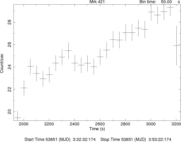$\begin{figure} \par\epsfig{file=0865fig2.ps,width=7cm,angle= -90} \end{figure}$	Figure 2: Light curve binned with 50 s intervals, from the first orbit of the 2006 April 26 pointing. Significant variability ( $\simeq$ $35\%$ ) is detected over intra-orbit time scale (1200 s).
Open with DEXTER

The fluxes were then dereddened using a value of E(B-V) equal to 0.014 mag (Schlegel et al. 1998) with $A_{\lambda}/E(B-V)$ ratios calculated for UVOT filters (for the latest effective wavelengths) using the mean Galactic interstellar extinction curve from Fitzpatrick (1999).

2.3 Swift-UVOT data analysis

We analysed the data that automatically triggered the BAT instrument (labelled with a (*) symbol in Table 1). To reduce the data we followed the instructions reported in the BAT analysis threads. We first generated a detector plane image (DPI) and checked for noisy pixels using the bathotpix task. To subtract the background effectively, we generated a weighting mask using the batmaskwtevt task. The spectrum was extracted using the batbinevt task. We applied geometric corrections (batupdatephakw), and systematic error corrections (batphasyserr). As a final task, we generated a response matrix (batdrmgen). The spectrum was rebinned by providing an external bin edge file to batbinevt.

3 Fast source variability

Temporal variability is one of the most interesting features characterizing HBLs. In the X-ray band, the typical timescales of flux changes decrease to the order of hour or minutes. The identification of the most rapid significant flux change allows us to estimate the source size, given by the well-known relation:

$\begin{displaymath} R \leq \frac{c~\Delta t~\delta}{1+z} , \end{displaymath}$

(1)

where c is the speed of the light, $\delta$ is the beaming factor, and z is the cosmological redshift. We investigated the intra-orbit light curves from our data set and found a significant flux variation in the first orbit observed on 2006 April 26 (ObsID 00030352006) pointing (see Fig. 2). The light curve extracted for the 0.3-10.0 keV band shows an increasing trend spanning about 1200 seconds with a variation of about $35\%$ .

According to Eq. (1), a 1200 s timescale implies that $R\leq 3.6\times 10^{13} \delta$ cm. Assuming a beaming factor approximately 10, we derive $R \simeq 4\times10^{14}$ cm, which is indicative of a compact emitting region.

Lichti et al. (2008) analysed the temporal variability of Mrk 421 using observations performed by the INTEGRAL-ISGRI instrument in the 40-100 keV band, and overlapping our data set during the June pointings. The most rapid variability observed in the INTEGRAL-ISGRI light curves, estimated by fitting the data with a rise-time law of the form $a\cdot {\rm e}^{t/t_0}$ , inferred that $R \la 3\times 10^{14} \delta$ cm. We performed the same analysis for the 2006 April 26 light curve and we found that $t_0\simeq 4.100$ s which implies $R \la 1\times 10^{14}\delta$ cm. We used this timescale to constrain the size of the emission region in the following analyses (Sect. 8).

Timescales of similar length of that in the 2006 April 26 pointing were also observed by Tanihata et al. (2001) in ASCA data, about 5 ks ( $R \la 1.5\times 10^{14}\delta$ cm), and by Giebels et al. (2007) (about 2 ks), who analysed TeV data from the CAT telescope ( $R \la 5.4\times 10^{13}\delta$ cm).

4 Spectral analysis

4.1 XRT spectral analysis

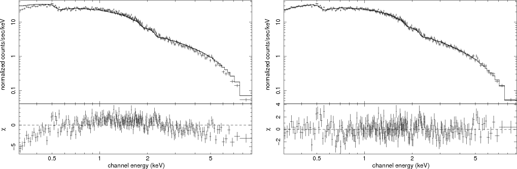$\begin{figure} \par\begin{tabular}{ll} \epsfig{file=0865fig3a.ps,width=5.6cm,an... ...psfig{file=0865fig3b.ps,width=5.6cm,angle=-90}\\ \end{tabular}\par \end{figure}$

Figure 3:

Spectrum from the first orbit of the ObsID 00030352013 performed on 2006 June 22. Left Panel: the systematic deviations on both sides of the residuals from a best fit with a power-law with Galactic $N_{\rm H}$ show the need of intrinsic curvature. Right panel: the deviations disappear with the log-parabolic model with Galactic $N_{\rm H}$ . The $\chi ^2_{r}$ decreases from 1.60 with 246 d.o.f. (power-law) to 1.19 with 245 d.o.f. (log-parabola); the F-test statistics clearly favours the curved model.

Open with DEXTER

For most spectra analysed, we detected systematic deviations (see Fig. 3) in the residuals obtained when fitting the data by means of a power-law spectrum with $N_{\rm H}$ fixed at the Galactic value. This behaviour implies heuristically that the spectra are intrinsically curved. This was known previously (Tanihata et al. 2004; Massaro et al. 2004; Tramacere et al. 2007b,a; Fossati et al. 2000b). All of these authors agreed that when the spectral shape of Mrk 421 is curved, can be difficult to describe its curvature in terms of absorption alone because this would require a column density much higher than the Galactic value of $N_H=1.61\times 10^{20}$ cm^-2 (Lockman & Savage 1995), and would also yield unacceptable fits of high $\chi ^2_{r}$ . Moreover, brightness profile derived from high resolution images of the host early-type galaxy of Mrk 421 do not exhibit any evidence of large amounts of absorbing material (Urry et al. 2000). Based on these phenomenological results, we performed the spectral analysis by fixing the $N_{\rm H}$ absorbing column densities to the Galactic values and using the following log-parabolic spectral law (LP):

$\begin{displaymath} F(E) = K~E^{-(a+b~\log(E))} ~~~~~~ \mbox{ ph cm$^{-2}$\space s$^{-1}$\space keV$^{-1}$ }, \end{displaymath}$

(2)

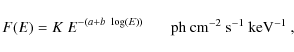
where a is the photon index at 1 keV and b measures the spectral curvature.

Both the SED peak energy ( $E_{\rm p}$ ) and height ( $S_{\rm p}$ ) can be derived easily from Eq. (2), but, in this case, they are affected by an intrinsic analytical correlation. This bias can be removed by using an equivalent functional relationship that is a log-parabola expressed in terms of $E_{\rm p}$ , $S_{\rm p}$ , and b (LPEP):

$\begin{displaymath} S(E)= (1.60 \times 10^{-9})~S_{\rm p}~10^{-b~(\log(E/E_{\rm p}))^2}~~~~~~\mbox{ erg cm$^{-2}$\space s$^{-1}$ }, \end{displaymath}$

(3)

where $S_{\rm p}=E_{\rm p}^2 F(E_{\rm p})$ and $E_{\rm p}$ are estimated during the fit, and the numerical constant is simply the energy conversion factor between keV and erg.

4.2 Orbit-resolved analysis

Because of the bright state of the source, we were able to extract spectra for each orbit, for a total of 172 spectra. A motivation for performing an orbit-resolved analysis is the strong variability of the source during these pointings. Integrating spectra over timescales much longer than the typical variability produces misleading results in estimating of the curvature, $E_{\rm p}$ , and $S_{\rm p}$ .

The results of the spectral analysis are reported in Table 2 (which is at the end of the text; rejected spectra are indicated by (*)), where all statistical errors refer to the $68\%$ confidence level (equal to one Gaussian standard deviation). The second, third, and forth columns in Table 2 report the best-fit parameters estimates for the model in Eq. (2). The fifth column reports the value of the SED peak estimated analytically from Eq. (2) according to the best-fit model results ( $E_{\rm p}*$ ). The sixth and seventh columns report the $E_{\rm p}$ and $S_{\rm p}$ best-fit model estimates using Eq. (3) as the best-fitting model. In the eighth column, we report the flux in the 0.3-10.0 keV band, evaluated by integrating the model function in Eq. (2). In the last column, we report the reduced $\chi^2$ statistics for the fit with Eq. (2).

The SED peak energy was often difficult to estimate. This was because during this particularly high brightness state, the spectra were in some cases hard, with a photon index of $a \simeq [1.6{-}1.7]$ and of low spectral curvature, implying a peak energy far from the XRT energy band.

To test the robustness of the $E_{\rm p}$ estimate, we first derived the peak energy from the spectral parameters of Eq. (2) ( $E_{\rm p}*$ ). We then fitted the spectra using Eq. (3), by setting the initial curvature value to that returned from the fit with Eq. (2). To test the stability of the results, we adopted the following criteria:

1.: The value of $E_{\rm p}$ is statistically significant. Given the asymmetric uncertainties, we define $\sigma_{E_{\rm p}}$ to be half of the 2 sigma confidence level, and require that $E_{\rm p}/\sigma_{E_{\rm p}}<1$ .
2.: $E_{\rm p}*$ consistent with $E_{\rm p}$ to a one sigma uncertainty .

We show in Table 2 the estimates of $E_{\rm p}$ satisfying this criterion, and in the other cases report only the lower limit of $E_{\rm p}*$ . The estimates of $E_{\rm p}*>100$ keV are obviously not statistically robust, meaning that the true energy peak may be in excess of 100 keV, although we are unable to provide a robust estimate.

All spectra for which the stability conditions were satisfied returned values of $E_{\rm p} \la 20$ keV.

4.3 Orbit-merged analysis

An orbit-resolved spectral analysis has the ability to follow accurately the strong variability in the source, even though the $E_{\rm p}$ estimates are affected by significant uncertainties. In any case, based on the spectral/flux pattern traced by the previous analysis, we can identify all the orbits indicating essentially the same spectral/flux states. We can use these intervals to perform an orbit-merged spectral analysis, and achieve smaller uncertainties in the $E_{\rm p}$ value, without integrating the source over periods that exhibits significant changes.

The results of this analysis are reported in Table 3 (which is at the end of the text). In this analysis, when $E_{\rm p}$ and $E_{\rm p}*$ can be determined, the typical uncertainties are smaller. We use the values from this table to perform $E_{\rm p}-S_{\rm p}$ and $E_{\rm p}-b$ trend analysis in the following sections, selecting only data with reliable $E_{\rm p}$ estimates. In this case, all spectra with $E_{\rm p}$ well-constrained have $E_{\rm p} < 20$ keV.

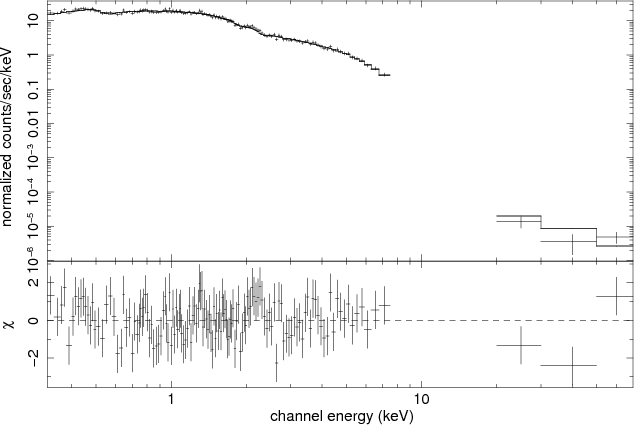$\begin{figure} \par\epsfig{file=0865fig4.ps ,width=6cm,angle=-90} \end{figure}$	Figure 4: Joint XRT BAT spectral analysis from the 2006 April 22 pointing.
Open with DEXTER

4.4 Joint XRT-BAT spectral analysis

For the three observations with simultaneous Swift-XRT and Swift-BAT data (with the BAT in automatic trigger mode, see Table 1), we performed a joint XRT-BAT spectral analysis. The results are reported in Table 3 (lines labelled X+B). The spectral curvature produced by the joint analysis is slightly larger than for the XRT data alone, but is always consistent within one sigma. As already discussed, the estimation of $E_{\rm p}$ is more difficult. We use the superscript ^X+B hereafter to refer to the joint XRT and BAT analysis.

For the 2006 15 July pointing, the two curvatures are $b=0.17\pm0.02$ and $b^{X+B}=0.20\pm0.02$ , and the two values of $E_{\rm p}$ which are consistent to within one confidence interval are $E_{\rm p}=11_{-2}^{+4}$ keV and $E_{\rm p}^{X+B}=8^{+2}_{-1}$ keV. For the case of the 2006 April 22 pointing (Fig. 4), the peak energies are $E_{\rm p}^{X+B}=20^{+10}_{-6}$ keV and $E_{\rm p}=26^{+19}_{-8}$ and the curvatures are $b=0.11\pm0.02$ and $b^{X+B}=0.12\pm0.02$ .

For the 2006 June 23 pointing, the XRT curvature is estimated to be $0.08\pm0.03$ which should be compared with the value of $b^{X+B}=0.13\pm0.02$ . In this case, the smaller the value of the curvature, as discussed in the previous section, the more difficult the estimate of the $E_{\rm p}$ value becomes. We found that the XRT data alone are unable to identify the true peak energy, and the estimate from our joint analysis is $E_{\rm p}^{X+B}=34^{+22}_{-11}$ keV.

The results of our joint XRT-BAT analysis confirm that $E_{\rm p}$ values estimated from XRT data, at energies higher than about 20 keV, are possibly biased. The selection applied to the present analysis should ensure that the bias affecting the trends between $E_{\rm p}$ , b, and $S_{\rm p}$ are as small as possible.

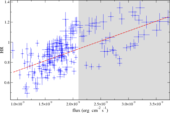$\begin{figure} \par\epsfig{file=0865fig5.ps,width=5.57cm,angle=-90} \end{figure}$	Figure 5: Scatter plot of the HR vs. the flux in the 0.2-10 keV band (HR is evaluated as the ratio of the 2.0-10.0 keV band to the 0.2-2.0 keV band). The points in the shaded area are almost all from the period 2006 June 23 to 2006 June 27 and 2006 July 15.
Open with DEXTER

5 Spectral evolution

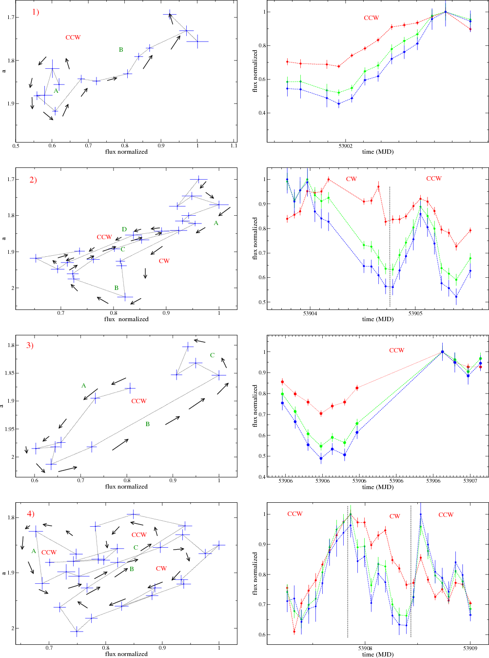$\begin{figure} \par\begin{tabular}{ll} \par\epsfig{file=0865fig6al.ps,width=5.5c... ... \epsfig{file=0865fig6dr.ps,width=5.5cm,angle=-90}\\ \end{tabular} \end{figure}$

Figure 6:

Left panels: spectral patterns in the a-flux plane showing clockwise and counterclockwise trends. Right panels: Swift-XRT light curves at three different bands: soft (0.2-3.0 keV, red), medium (3.0-5.0 keV, green), and hard ( 5.0-10.0 keV, red) . Capital letters guide the reader during the comment in the text. In both left and right panels, the fluxes are normalized to the maximum value reached during that particular time-interval.

Open with DEXTER

We now complete a classical hardness-ratio (HR) analysis, to investigate cooling and/or acceleration features. The HR is evaluated as the ratio of the flux measured in the 2.0-10.0 keV band to that in the 0.2-2.0 keV band.

An analysis of the evolution in the HR indicates that the correlations between variations in the soft and hard bands modulates the HRs, producing spectra that are harder when the source is brighter and softer when it is weaker. This trend is clearly visible in Fig. 5. The significant scatter in the data points implies that the evolutions of the flares are different from each other due to the different underlying physical conditions.

We also note that all but 3 of the data points in the shaded area belong to the period from 2006 June 23 to 2006 June 27 and to the 2006 July 15 pointing, when the source was brighter than in the previous pointings.

A deeper understanding of the spectral evolution can be achieved by analysing the hysteresis patterns of the single flares in the a-flux or HR-flux plane, where a is the photon index at 1 keV (see Table 2).

The timescales relevant to understanding the patterns in the a-flux plane are those of injection ( $\tau_{\rm inj}$ ), escape ( $\tau_{\rm esc}$ ), cooling ( $\tau_{\rm cool}$ ), acceleration ( $\tau_{\rm acc}$ ) and light crossing ( $\tau_{\rm cross}$ ) time. According to Kirk et al. (1998), the loops are expected to be clockwise (CW) and have soft lag when the flare is observed at frequencies where the higher energy variability occurs more rapidly than at lower energy (as in the case of synchrotron cooling). In contrast, when observed at frequencies for which the acceleration and cooling timescale are almost equal, the loops are expected to be counter-clockwise (CCW) with a possible hard lag.

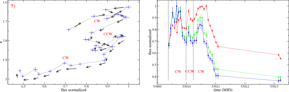$\begin{figure} \par\begin{tabular}{ll} \epsfig{file=0865fig7dl.ps,width=5.5cm,an... ... \epsfig{file=0865fig7dr.ps,width=5.5cm,angle=-90}\\ \end{tabular} \end{figure}$

Figure 7:

Left panels: spectral patterns in the a-flux plane showing clockwise and counterclockwise trends. Right panels: Swift-XRT light curves at three different bands: soft (0.2-3.0 keV, red), medium (3.0-5.0 keV, green), and hard ( 5.0-10.0 keV, red) . Capital letters are referenced in the discussion in the text. In both left and right panels, the fluxes are normalized to the maximum value reached during that particular time interval.

Open with DEXTER

We investigated carefully all the patterns from our data-set, and in Figs. 6 and 7 we report the 5 flares showing a clear CW or CCW loop. The left panels show the evolution of a as a function of the flux, and the right panels show the light curves in three different bands. The fluxes are normalized to the maximum value reached in that particular time interval. As a general result, we did not find any significant plateau among the light curves of these flares, which implies that $\tau_{\rm inj}<\tau_{\rm cross}$ . We describe the behaviour of the flares individually:

Flare 1): the flare has a CCW pattern; it begins with a softening of the spectrum with a flux almost steady (A) probably reflecting the cooling from the previous flaring episode, followed by a flux increase with a spectral hardening (B);
Flare 2): the flare has two patterns: one CW and one CCW. It starts with a decreasing flux and a spectral softening (A) ( $\tau_{\rm cool} \ll \tau_{esc}$ ). Figure 6 (left panel) shows that the flux in the soft band is still increasing when the fluxes in the medium and hard bands are already decreasing. When the spectrum starts to become harder (B), the flux is still decreasing, which may imply that we are seeing the propagation of the new injection from the hard band, as the soft band is still decreasing. The flux then starts to increase with the spectrum hardening (C). When the flare begins to decay (D) the pattern switches to CCW and we witness a decrease in the flux and a spectral softening;
Flare 3): the flare has a CCW pattern, starts with a flux decrease and a spectral softening (A), then the flux increases and the spectrum hardens (B). In the last part (C), the flux decreases and the spectrum still hardens. As in the previous case this may hint the start of a new hard flaring component;
Flare 4): this flare has three patterns: CCW, CW, and CCW. It starts with a CCW loop. Initially, there is a spectral change with an almost steady flux (A), followed by a weak spectral hardening with a flux increase (B). The CW loop is dominated by the cooling time. The final CCW pattern is characterized by a flux increase and a rapid spectral hardening. In this case, the new flaring component also seems to start in the hard band. The flux decrease (C) is almost achromatic in this case, and the escape time may dominate over the cooling one ( $\tau_{\rm esc} \ll \tau_{\rm cool}$ );
Flare 5): this flare has three patterns: CW, CCW, and CW. It does not have features that differs from those of other patterns.

CW loops were studied for the same source by Takahashi et al. (1996) with ASCA observations. Zhang (2002) observed CCW using BeppoSAX observations on 21 April 1998. Similar types of loops were also observed in PKS2155-304 by Kataoka et al. (2000) and 1H1426+428 by Falcone et al. (2004).

6 Spectral parameter trends

We compare the trends between the spectral parameters with those detected in the statistical analysis of Tramacere et al. (2007b). We extend the data set presented in that work with the results from the observations analysed in this paper. We note that this entire data set spans about ten years, sampling the source in different brightness states and making the final result more statistically significant.

6.1 E ${_{\rm p}}$ - b trend

The evolution in the curvature parameters as a function of the peak energy highlights the features relevant to the acceleration process. This analysis indicates that as the peak energy of the emission increases, the cooling timescale shortens and can compete with the timescales for acceleration, it is then possible to observe a bias in the $E_{\rm p}-b$ relation, because the cooling timescale are shorter than the timescales for acceleration.

We analysed the data in Table 3, identifying cooling-dominated observations (lines labelled with (c)), characterized by a strong flux decrease and strong spectral softening ( $a\simeq2$ ). In Fig. 8, we plot with green empty circles the whole XRT data set from Table 3 and with black squares the points without the strong cooling contamination discussed above.

In the same figure, we also report data from Tramacere et al. (2007b), showing that the trend in our sample is consistent with that from the historical data. This agreement confirms that the spectral curvature decreases as $E_{\rm p}$ moves toward higher energies.

This phenomenon can be interpreted by two different scenarios. A first scenario is that of an energy-dependent acceleration probability process (EDAP). Within this context, Massaro et al. (2004) showed that when the acceleration efficiency is inversely proportional to the energy itself, the energy distribution approaches a log-parabolic shape. According to this model, the curvature (r) is related to the fractional acceleration gain ( $\varepsilon$ ) by $r\propto \frac{1}{\log ~ \varepsilon}$ . A possible example is given by particles confined by a magnetic field, whose confinement efficiency ( $P_{\rm acc}$ ) decreases as the gyration radius (R_L) increases. From $E_{\rm p}\propto \varepsilon$ and $r\propto \frac{1}{\log \varepsilon}$ , the negative trend between $E_{\rm p}$ and b follows. This trend is in agreement with the observed trend.

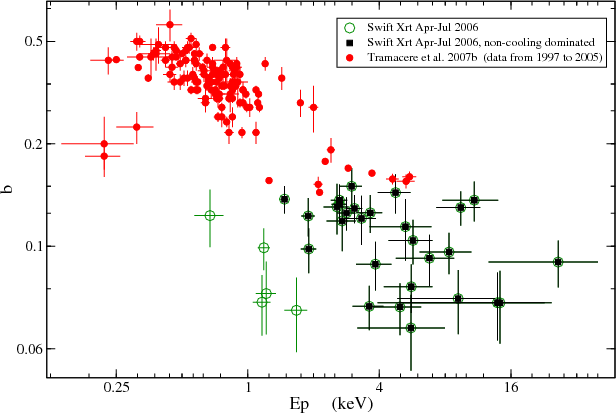$\begin{figure} \par\epsfig{file=0865fig8.ps,width=6cm,angle=-90} \end{figure}$	Figure 8: Scatter plot of the curvature (b) vs. $E_{\rm p}$ . Red circles represent data from Tramacere et al. (2007b) spanning from 1997 to 2005, instruments: ASCA, BeppoSAX, XMM-Newton. Black boxes represent Swift data from the present analysis without the cooling-dominated events. Empty green circles represent the whole XRT data set presented in this paper.
Open with DEXTER

An alternative explanation is provided by the stochastic acceleration framework (SA) and the presence of a momentum-diffusion term. In this scenario, the diffusion term acts on the electron spectral shape broadening the distribution. In particular, Kardashev (1962) showed that a log-parabolic spectrum results from a Fokker-Planck equation with a momentum-diffusion term and a monoenergetic or quasi-monoenergetic particle injection. The results presented in Tramacere et al. (2007b) rely on the theoretical prediction from the Kardashev (1962) model, that the curvature term (r) is inversely proportional to the diffusion term (D):

$\begin{displaymath} r \propto\frac{1}{Dt}\cdot \end{displaymath}$

(4)

This relation leads to the following trend between the peak energy of the electron distribution ( $\gamma_{\rm p}$ ), the synchrotron curvature (b=r/5), r, and $E_{\rm p}$ :

$\begin{displaymath} \ln(E_{\rm p})= 2\ln(\gamma_{\rm p})+3/(5b). \end{displaymath}$

(5)

In Paper II (Tramacere 2009) we will discuss in detail how the stochastic acceleration can be used to reproduce this trend by developing a physical scenario that fits these phenomenological results. Here, we remark that both the momentum-diffusion term D and, the fractional acceleration gain $\varepsilon$ can explain the anticorrelation observed between $E_{\rm p}$ and b.

6.2 S ${_{\rm p}}$ (L ${_{\rm p}}$ ) - E ${_{\rm p}}$ trend

In terms of the synchrotron emission the trend between $S_{\rm p}$ and $E_{\rm p}$ has implications for the driver of the spectral changes in the X-rays. This trend can be used to understand how the luminosity of the jet evolves as the particle energy increases. In the framework of the synchrotron theory (Rybicki & Lightman 1979), the dependence of $S_{\rm p}$ on $E_{\rm p}$ can be expressed in the form of a power-law:

$\begin{displaymath}S_{\rm p} \propto E_{\rm p}^{\alpha}. \end{displaymath}$

(6)

Starting from the following functional relation, the SED peak height reads:

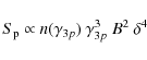$\begin{displaymath}S_{\rm p} \propto n(\gamma_{3p})~\gamma_{3p}^{3}~B^2~\delta^4 \end{displaymath}$

(7)

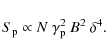
and the peak energy is given by:

$\begin{displaymath}E_{\rm p} \propto \gamma_{3p}^2B~\delta \end{displaymath}$

(8)

where $\gamma_{3p}$ is the peak of $n(\gamma)~\gamma^{3}$ , B the magnetic field, and $\delta$ is the beaming factor.

If we take into account a log-parabolic distribution for the electrons emitting the X-ray photons, then it is easy to show that the total emitters number $N=\int n(\gamma)d\gamma \simeq n(\gamma_{\rm p})~\gamma_{\rm p}$ , with $\gamma_{p}$ the peak of $n(\gamma)~\gamma$ . This in terms of $S_{\rm p}$ , implies that

$\begin{displaymath}S_{\rm p} \propto N~\gamma_{\rm p}^{2}~B^2~\delta^4. \\ \end{displaymath}$

(9)

Thus $\alpha=1.0$ applies when the spectral changes are dominated only by variations in the electron average energy and N is constant, $\alpha=1.5$ applies when the spectral changes are dominated by variations in the average electron energy but N is not constant; $\alpha=2$ relates to changes in the magnetic field; $\alpha=4$ if changes in the beaming factor dominate; formally, $\alpha=\infty$ applies to changes only in the number of emitting particles, which implies either a change in the electron density or a change in the source size. The case $\alpha=1.0$ holds only if the electron distribution is a log-parabola and if the curvature is constant.

To obtain a deeper understanding of the relation to the jet energetics, we plot on the y axis of Fig. 9, $L_{\rm p}= S_{\rm p}~4\pi~ D_L^2$ , where $D_L\simeq 134.1$ Mpc is the luminosity distance. We report the $L_{\rm p}$ values both in Tables 2 and 3. The resulting scatter-plot represents the $L_{\rm p}-E_{\rm p}$ trend obtained from merging our data sample with that from Tramacere et al. (2007b). We fitted the data by means of a simple power law (PL) $L_{\rm p} \propto E_{\rm p}^{\alpha}$ , and a broken power-law (BPL)

$\displaystyle L_{\rm p}$	$\textstyle \propto$	$\displaystyle E_{\rm p}^{\alpha_1},~~~~ E_{\rm p} \leq E_b$	(10)
$\displaystyle L_{\rm p}$	$\textstyle \propto$	$\displaystyle E_{\rm p}^{\alpha_2},~~~~ E_{\rm p} > E_b.$

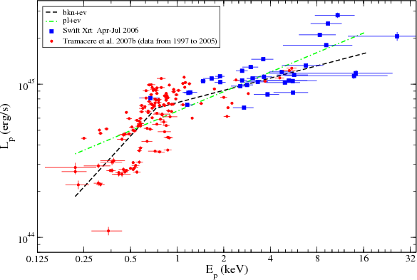The simple power-law fit gives a value of $\alpha=0.42\pm 0.06$ , and the broken power law gives a break energy $E_b=1\pm 1$ keV, with two slopes of $\alpha_1=1.1\pm 0.2$ and $\alpha_2=0.27\pm 0.07$ .

$\begin{figure} \par\epsfig{file=0865fig9.ps,width=5.6cm,angle=-90} \end{figure}$	Figure 9: Scatter plot of $L_{\rm p}$ vs. $E_{\rm p}$ . Red circles represent data from Tramacere et al. (2007b) spanning from 1997 to 2005, instruments: ASCA, BeppoSAX, XMM-Newton. Blue boxes represent Swift data from the present analysis. The dashed dotted line represents the best fit using a power-law and the dashed line represents the best fit using a broken power law.
Open with DEXTER

We focus on the results from the BPL fit. Although the break energy is not well constrained, we note that spectral slopes differ with a high statistical significance. This break in the trend implies that for $E_{\rm p}\la 1$ keV and $L_{\rm p}\la 10^{45}$ erg/s, the driver follows the relation with $\alpha \simeq 1.0$ (we define this state the quiescent sate), whilst for $E_{\rm p} \ga 1$ keV and $L_{\rm p} \ga 10^{45}$ erg/s, the driver relates to $\alpha \simeq 0.2$ (we define this to be the high state).

In Paper II (Tramacere 2009), we will discuss in detail how the stochastic acceleration or the energetics of the jet can be used to reproduce this trend.

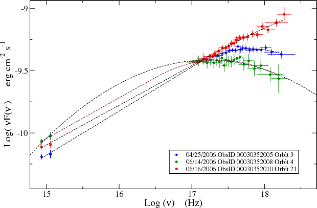$\begin{figure} \par\epsfig{file=0865fig10.ps,width=6.5cm,angle=-90} \end{figure}$

Figure 10:

Three different spectral shapes from the data presented in this paper. Red boxes represent a power-law spectrum observed during Orbit 3 (ObsID 00030352010) on 2006 June 16. Blue diamonds represent a spectrum that is a log-parabola with a low energy power-law tail, from Orbit 3 (ObsID 00030352005) on 2006 April 25. Green circles represent a log-parabolic spectrum from Orbit 4 (ObsID 00030352008) on 2006 June 14.

Open with DEXTER

7 The Swift-UVOT Swift-XRT connection: the low-energy power-law tail in the electron distribution

Both the $E_{\rm p}-b$ and $S_{\rm p}-E_{\rm p}$ trends allowed us to understand the shape of the electron distribution for particles emitting at energies close to $E_{\rm p}$ . The particle energy distribution can develop a low energy shape that differs from the extrapolation of the high energy branch. This difference is relevant in discriminating between different acceleration processes. In this perspective, the connection between the UV and X-ray spectra can provide useful information about the low energy tail of the electrons emitting in the X-ray. We analysed carefully all of the spectra with simultaneous X-ray and UV observations. As a result, we found that joint UVOT-XRT SEDs can be classified in three categories:

a)

described by a log-parabola (LP)

b)

described by a power law (PL)

c)

described by a spectral law that is a power law at its low energy tail, becoming a log-parabola function at its high energy one (LPPL) (Massaro et al. 2006), whose functional form can be expressed by

$\displaystyle \nu~F(\nu)$	=	$\displaystyle N~(\nu/\nu_c)^{-a_{\nu}},~~~~~~~~~~~~~~~~~ \nu \leq \nu_c$
$\displaystyle \nu~F(\nu)$	=	$\displaystyle N~(\nu/\nu_c)^{-(a_{\nu}+b~\log(\nu/\nu_c))} , \nu >\nu_c .$	(11)

where $a_{\nu}$ is the spectral index of the SED ( $\nu~F(\nu)$ ), and $\nu_c$ is the frequency at which the turn-over in the SED occurs (Fig. 10).

From the analysis of this spectral behaviour, it is possible to constrain the minimum energy of the radiating electrons. Electrons radiating mainly in the UV band have a Lorentz factor $\gamma_{UV}$ satisfying the following condition (Rybicki & Lightman 1979):

$\displaystyle 10^{15} \mbox{ Hz}$	$\textstyle \simeq$	$\displaystyle 3.7\times10^{6}~B~\delta~{\gamma_{UV}}^2/(1+z)$	(12)
$\displaystyle \gamma_{UV}$	$\textstyle \simeq$	$\displaystyle 1.6 \times10^{4} \sqrt{\frac{1+z}{B~\delta}} \cdot$

If the spectral shape is consistent with the same log-parabola extending from the X-ray band down to the UV band (case a), then it means that electrons radiating at UV frequencies belong to the same electron population and according to Eq. (12), we have $\gamma_{\rm min} \lesssim \gamma_{UV}$ .

The condition $\gamma_{\rm min} > \gamma_{UV}$ may occur when we observe a PL (case b) or a LPPL (case c). If $\gamma_{\rm min} > \gamma_{UV}$ , then the spectra in the X-ray-to-UV band will be described by the asymptotic low-energy approximation of the single particle synchrotron emission that is a power law with slope $a_{\nu}\simeq{-4/3}$ ( ${\it SED} \propto\nu^{4/3}$ ) (Rybicki & Lightman 1979).

For both cases b) and c) we note that our data infer $a_{\nu}\simeq[0.25{-}0.4]$ , a value that differs significantly from the asymptotic synchrotron kernel expectation. This implies that in both cases the UV photons probably are emitted by an electron distribution that has a power-law tail in the energetic range radiating in the UV-to-soft-X-ray band. A phenomenological option to explain the case c) is an electron distribution that is a power law at low energies with a log-parabolic high-energy branch (LPPL) (Massaro et al. 2006):

$\displaystyle n(\gamma)$	=	$\displaystyle K~(\gamma/\gamma_c)^{-s},~~~~~~~~~~~~~~~~~ \gamma \leq \gamma_c$
$\displaystyle n(\gamma)$	=	$\displaystyle K~(\gamma/\gamma_c)^{-(s+r~{\rm Log}(\gamma/\gamma_c))} , \gamma >\gamma_c ,$	(13)

where $\gamma_c$ is the turn-over energy.

In the case b), the electron distribution is assumed to be a pure power-law.

Interestingly for case b) and case c), we can also constrain the typical slope of the power-law branch of the electron distribution, using the well-known relation between the spectral index in the particle distribution s and that in the SED (Rybicki & Lightman 1979):

$\begin{displaymath}SED \propto \nu^{-a_{\nu}}=\nu^{-(s-3)/2}. \end{displaymath}$

(14)

For the typical values of $a_{\nu}$ observed in our data set, the resulting value of s is in the range $s\simeq[2.2{-}2.5]$ .

The presence of a power-law feature and the range of observed spectral indices are relevant both in the context of Fermi first-order acceleration models and from an observational point of view.

From the observational side, we note that Waxman (1997) and Mészáros (2002), studying the the afterglow X-ray emission of $\gamma-$ ray bursts (GRB), inferred an electron distribution index of $s\simeq 2.3 \pm 0.1$ . This is close to those found in our data, but corresponds to a quite different class of sources.

From a theoretical point of view, several works study relativistic-shock acceleration models that start from different analytical or numerical approaches and find values of $s \simeq [2.2-2.4]$ (Ellison & Double 2004; Achterberg et al. 2001; Gallant et al. 1999; Blasi & Vietri 2005; Lemoine & Pelletier 2003). These values are consistent with those from our data set.

The power-law feature is also consistent with a purely stochastic scenario. The usual limitation of the stochastic model to explain a universal index relies on the fine tuning required to the ratio of the acceleration timescale to the loss time ( $s\simeq 1+t_{\rm acc}/t_{\rm esc}$ ), to reproduce the observed values.

We stress that a power-law electron distribution $n(\gamma) \propto \gamma^{-2.3}$ is inconsitent with a Maxwellian-like distribution ( $n(\gamma) \propto \gamma^{2}$ ) resulting from the equilibrium of SA processes without relevant particle escape.

In conclusion, both cases c) and b) are explained more accurately by a first order process. We will discuss this topic further in Sect. 9.

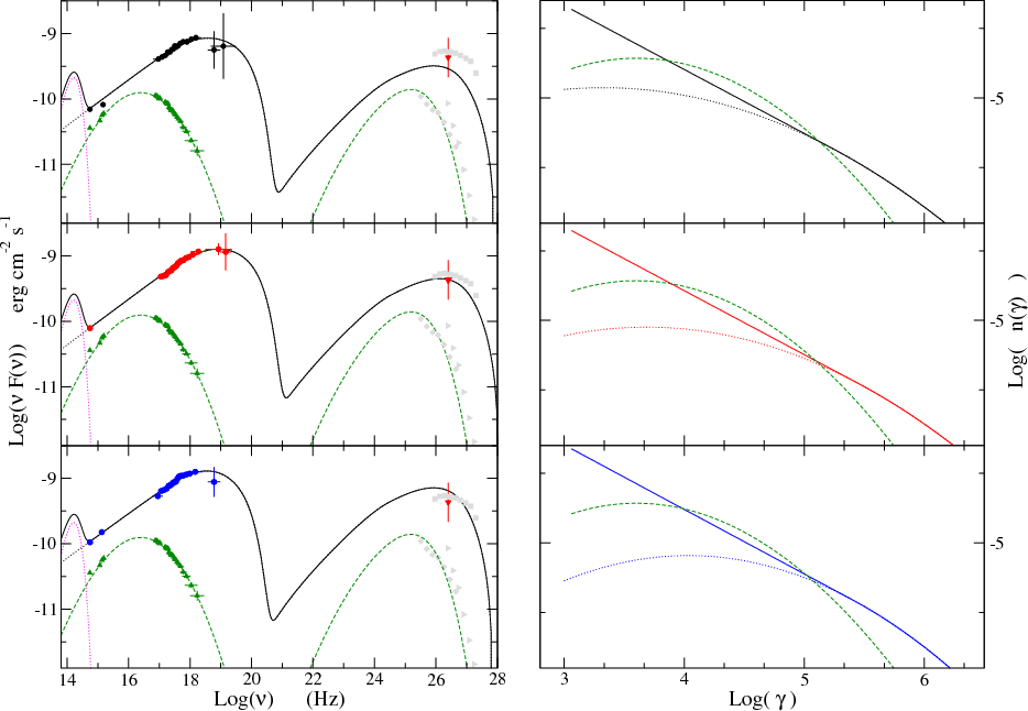$\begin{figure} \par\begin{tabular}{ll} \epsfig{file=0865fig11l.ps,width=7.8cm,an... ...} &\epsfig{file=0865fig11r.ps,width=7.8cm,angle=0}\\ \end{tabular} \end{figure}$

Figure 11:

SSC fits of three different observations with simultaneous UVOT XRT and BAT data. Left panels show the SSC model, from top to bottom: solid circles represent data from 2006 April 22, 2006 June 23, and 2006 July 15 Swift observations. Green triangles show Swift-XRT data on 2005 March 31 from Tramacere et al. (2007b). Solid grey polygons represent non-simultaneous EBL corrected TeV data. Solid gray squares represent the high state on 2001 observed by Whipple, data from Albert et al. (2007). Solid gray diamonds represent the average 2004-2005 TeV spectrum as observed by MAGIC (Albert et al. 2007). Solid gray right triangles represent the average spectrum from December 2005 to February 2006 as observed by TACTIC (Yadav et al. 2007). The solid red triangle represents a Whipple observation on June 18, 19, 21 from Lichti et al. (2008), that is very close in time to our 2006 June 23 data set. The solid lines represent the best fit by a SSC model to our simultaneous Swift observation, and the dashed line is the best SSC fit to the Swift data on 03/31/2005. The dotted lines represent the modelling of the galaxy contribution by means of black body spectral shape. Right panels show the electron distributions for the SSC models in the left panels. The solid lines in the right panels represent the electron distributions for the best fit models of the three 2006 Swift observations, the dotted lines represent the extrapolation of the LP branch of the LPPL distribution, and the dashed lines represent the electron distribution for the 2005 March 31 data.

Open with DEXTER

Table 4: SSC best-fit model results for the 2006 Swift observations and using as electron distribution a log-parabola with a power-law low-energy branch (Eq. (13)).

Table 5: SSC best fit results for 2005 March 31 Swift observation and using a log-parabolic electron distribution as defined in Eq. (15).

8 SED modelling and GeV/MeV predictions

We model the SEDs of three observations with simultaneous XRT, BAT , and UVOT data, using a standard one-zone SSC scenario. The only useful TeV data found in the literature are from Whipple observations on June 18, 19, and 21 (Lichti et al. 2008). Almost simultaneous only with the 06/23/2006 Swift pointing, these data provide only the TeV flux, without giving a description of the spectrum. For this reason, they are only used to estimate the TeV flux level during that pointing.

To estimate the spectral and flux range of variability, we also plot Swift-XRT data from 2005 March 31 (Tramacere et al. 2007a), and some TeV SEDs representing the source in different flaring states (Yadav et al. 2007; Albert et al. 2007) (see left panel of Fig. 11).

The 2006 SEDs that we want to model have a power-law spectral dependence between the UVOT and XRT bands. As described in Sect. 7, the most generic distribution accounting for this spectral shape is a power-law at low energy with a log-parabolic high-energy branch (Eq. (13)). In contrast, the 2005 March 31 SED can be modelled using a log-parabolic electron distribution that we express in terms of the peak energy as (LPEP):

$\begin{displaymath}n(\gamma)= K~10^{-r~(\log(\gamma/\gamma_{\rm p}))^2}. \end{displaymath}$

(15)

Since we do not know the true shape and flux at TeV energies (we have only an estimate of the flux at $\simeq$ 1 TeV), we cannot constrain in detail the SSC model using the canonical $B-\delta$ plane analysis (Tavecchio et al. 1998). However, we can still use the results reported in Sects. 3 and 7 to constrain some of the SSC parameters.

The first constraint comes from the source variability (see Sect. 3):

$\begin{displaymath}R/\delta \leq 1 \times 10^{14} ~\mbox{cm}. \end{displaymath}$

(16)

A second constraint comes from the analysis of the UVOT connection with the XRT data that provides an upper limit to $\gamma_{\rm min}$

$\begin{displaymath}\gamma_{\rm min} \la 1.6 \times10^{4} \sqrt{\frac{1+z}{B~\delta}}\cdot \end{displaymath}$

(17)

To constrain the value of the maximum electron energy, we can use the maximum energy of the synchrotron emission, taking as the corresponding energy the most energetic bin of the BAT detector with a significant signal ( $\simeq$ 50 keV)

$\begin{displaymath}\gamma_{\rm max} \gtrsim 1.8 \times10^{6} \sqrt{\frac{1+z}{B~\delta}} \cdot \end{displaymath}$

(18)

A further constraint on $\gamma_{\rm max}$ can be set by estimating the typical electron energy required to produce TeV photons (Bednarek & Protheroe 1999). Based on the historical data for Mrk 421, the spectrum typically reaches 10 TeV, and this implies that

$\begin{displaymath}\gamma_{\rm max} \gtrsim 2\times 10^7 \frac{1+z}{\delta}\cdot \end{displaymath}$

(19)

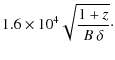
Following Bednarek & Protheroe (1999) and combining Eqs. (19) and (18), we obtain an upper limit to the magnetic field:

$\begin{displaymath} B/\delta \la 0.008 ~ \textnormal G. \end{displaymath}$

(20)

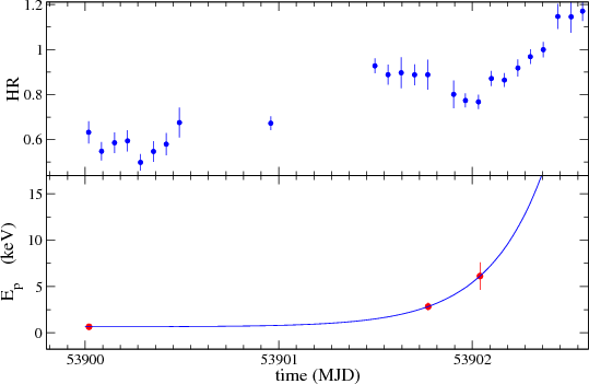The best-fit model was obtained by combining our numerical SSC code (Tramacere 2007) with a numerical minimizer. According to the observationally derived constraints, we fixed the value of the beaming factor to $\delta=25$ , the magnetic field to B=0.1 G, the source size to $R=2.1\times10^{15}$ cm, and tuned to $\gamma_{\rm min}=1100$ to obtain the correct Compton dominance, leaving $r,~s,~\gamma_c$ , $\gamma_{\rm max}$ , and N as free parameters. The resulting best-fit model parameters are reported in Tables 4 and 5.

$\begin{figure} \hspace*{4mm}\epsfig{file=0865fig12.ps ,width=5.6cm,angle=-90} \end{figure}$	Figure 12: Lower panel: the increase of $E_{\rm p}$ during a flare starting on 2006 June 14, fitted by an exponential function. Upper panel: the corresponding HR.
Open with DEXTER

In the left panels of Fig. 11 we show the best-fit model results for the SSC model for the 2006 data and for the 2005 March 31 pointing. In the right panels, we show the corresponding electron distributions. The values of the electron curvature are consistent with those observed in the X-ray emission according to the relation $b\simeq r/5$ . The typical value of the ratio $u_e/u_B \simeq [120{-}180]$ corresponds to that in a particle-dominated jet agreeing with the typical values for TeV HBLs peaking in the hard X-ray (Kino et al. 2002; Sato et al. 2008). The low-energy power-law branch of the electron energy distribution follows $n(\gamma) \propto \gamma^{-2.3}$ , in agreement with the analysis presented in Sect. 7.

We note that UV data are weakly contaminated by the host-galaxy emission.

In the left panel of Fig. 11, we plot the contribution of the galaxy emission modelled as a black-body spectral shape (dotted-line). This plot clearly shows how the UVOT data considered lie beyond the galaxy emission spectral cut-off. In contrast, during the low states, the possible power-law tail would lay typically at optical and lower frequencies, where the emission is typically dominated by the galaxy. This implies that we are unable to determine whether the electron distribution also has a power-law tail during the lower state. The SED model of data on 2005 March 31 shows that the UVOT points are consistent with the synchrotron emission from a log-parabolic electron population.

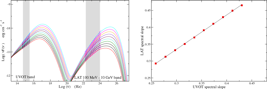$\begin{figure} \par\begin{tabular}{ll} \epsfig{file=0865fig13l.ps ,width=5cm,ang... ... &\epsfig{file=0865fig13r.ps ,width=5cm,angle=-90}\\ \end{tabular} \end{figure}$

Figure 13:

The strong correlation between the UVOT spectral slope and that in the LAT band for a SSC scenario. In the left panel we show the SSC SEDs and in the right panel we show the correlation between the spectral slope in the UVOT band and that in the Fermi- LAT band. Basic parameters for the SSC model are: particle number density $N=10 ~\mbox{cm}^{-3}$ , magnetic field intensity B=0.1 G, minimum electron energy $\gamma _{\rm min}=10^3$ , maximum electron energy $\gamma _{\rm max}=5\times 10^6$ , emitting region radius $R=3.0\times15~\mbox{cm}$ , beaming factor $\delta =15$ , electron curvature r=1.0, power law of index of the low-energy tail of the electron distribution s=[2.2:2.5], and turn-over energy in the electron distribution $\gamma _c=5.0\times 10^4$ .

Open with DEXTER

If present in the 2005 SED, a power-law low-energy branch would yield an index harder than those from 2006, but of much lower flux.

Another interesting analysis can be performed by looking at the acceleration timescales determined by the rate of the variation in E_P. In particular, we can use the e-folding time of $E_{\rm p}$ to infer the electron acceleration timescale $\tau_{\rm acc}$ . From $E\propto \gamma^2$ , it follows that the rate of change in $E_{\rm p}$ can be related to the rate of change in $\gamma$ for electrons radiating in the hard X-ray band. In Fig. 12, we show a flare with well constrained values of $E_{\rm p}$ for the rising side. In this figure, we plot the values of $E_{\rm p}$ as a function of time. The e-folding time for $E_{\rm p}$ results in a $\gamma$ e-folding time of about 0.15 days, which is the value of the typical acceleration timescale. This is the timescale that will compete with the cooling one to generate the equilibrium in the $n(\gamma)$ distribution. In particular, taking into account the synchrotron cooling:

$\begin{displaymath}\tau_{\rm cool}\simeq 10^8/(B^2\delta\gamma) ~~ \mbox{s} \end{displaymath}$

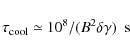(21)

the equilibrium of the distribution for a log-parabolic or Maxwellian-like distribution is the peak of $n(\gamma)$ . In the case of LPPL distribution, it will be constrained between $\gamma_c$ and $\gamma^{\rm LP}_{\rm p}$ . Imposing $\tau_{\rm cool}=\tau_{\rm acc}$ we find:

$\begin{displaymath}\gamma_{eq}=\frac{10^8}{\tau_{\rm acc}~B^2\delta} \end{displaymath}$

(22)

For $\tau_{\rm acc}\simeq 0.15$ days, $\delta=25$ and using $\gamma_{\rm eq}$ of the order of 10⁴, the resulting value of the magnetic field is

$\begin{displaymath}B=\sqrt{\frac{10^8}{\tau_{\rm acc}\delta\gamma_{\rm p}}}\simeq 0.16~ \mbox{G}, \end{displaymath}$

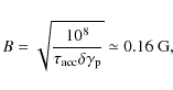(23)

which is consistent with the upper limit of Eq. (20) and with our best-fit model field strength.

8.1 The connection between the UV slope and that at MeV/GeV energies

An important consequence of the spectral shape in the UV band is due to the connection with the shape expected at MeV/GeV energies, and in particular in the Fermi Gamma-ray Space Telescope-LAT band.

To explore this, we simulated SSC emission by accounting for a typical HBL SED. As the electron distribution, we used a power-law at low energy with a log-parabolic high energy branch (LPPL) (Eq. (13)). The SSC parameter are reported in the caption of Fig. 13. In the left panel of this figure, we show different SEDs obtained by varying the s parameter in the range [2.1:2.5], and in the right panel, we show how the spectral shape in the UVOT band is tightly correlated with that in the Fermi-LAT energy range. This means that a comparison between the two spectral slopes derived from simultaneous observations can help us to determine whether the UV photons from the same component emitting in the X-ray are also responsible for the SSC emission.

9 Discussion

We have analysed the spectral and flux evolution of Mrk 421 during Swift observations between April and July 2006 , with the June pointings monitoring the source almost continuously for 12 days. During this period, the source exhibited both flux levels and SED peak energies each equal to their historic maximums until 2006. This very intense flaring state of Mrk 421 represented a unique opportunity to test the correlations among the spectral parameters presented in previous works (Tramacere et al. 2007b), increasing the temporal extent to about 10 years and enlarging the volume of the parameter space.

The spectral evolution of the source and the patterns in the a-flux plane (Sect. 4) suggest that each flare had a different characterization in terms of competition between the relevant timescales. Some flares showed a rise in the hard and medium X-ray band much faster than observed in the soft X-rays. This behaviour is probably due to the flaring component starting in the hard X-ray band and implies that the driver of those flares is the rapid injection of very energetic particles rather than a gradual acceleration.

The $S_{\rm p}-E_{\rm p}$ and $E_{\rm p}-b$ trends follow those presented in Tramacere et al. (2007b), where $E_{\rm p}$ and $S_{\rm p}$ are correlated, and $E_{\rm p}$ , b anti-correlated. These trends are relevant in understanding the physical mechanisms driving the evolution of the electron distribution under the effect of acceleration processes and may represent a common scenario for HBLs. Massaro et al. (2008) confirmed that the $E_{\rm p}-b$ relation holds for five of the TeV HBLs included in their analysis (PKS 0548-322, 1H 1426+418, Mrk 501, 1ES 1959+650, PKS 2155-304)), and that, as for the $S_{\rm p}-E_{\rm p}$ relation, the only exception to the previous list is PKS 2155-304.

The $E_{\rm p}-b$ relation shows a possible signature of acceleration processes that produce curved electron distributions, where the curvature decreases as the acceleration becomes more efficient. A first consistent with these results is an energy-dependent acceleration probability process (Massaro et al. 2004). An alternative explanation is provided by the stochastic acceleration framework and the presence of a momentum-diffusion term (Tramacere et al. 2007b; Kardashev 1962). Both scenarios predict a negative correlation between $E_{\rm p}$ and b and are consistent with the the data plotted in Fig. 8. We note that the data presented here cover a significant range of the parameter space, confirming that the relation between the curvature and the peak energy follows the same trend between the faintest and the strongest flaring activity, implying that the acceleration process remains the same.

A future investigation may be focused on understanding which physical parameters control the acceleration process. An interesting investigation may be the connection of the stochastic scenario with the turbulence spectrum of the MHD waves and of the resulting diffusion coefficient (Katarzynski et al. 2006; Park & Petrosian 1995; Stawarz & Petrosian 2008; Becker et al. 2006). Understanding the role of both the turbulence spectrum and, in general, the fluctuation in the particle energy gain is a complex task and requires a more detailed analysis that is beyond the purpose of this paper and will be presented in Paper II (Tramacere 2009).

The $S_{\rm p}-E_{\rm p}$ trend demonstrates the connection between the average energy of the particle distribution and the power output of the source. Compared with the observed values of $\alpha$ , the expected power-law dependence $S_{\rm p}\propto~E_{\rm p}^{\alpha}$ excludes $B, \delta$ and N, indicating $\gamma_{\rm p}$ as the main driver of the $S_{\rm p}-E_{\rm p}$ trend, confirming the result from Tramacere et al. (2007b). A more detailed analysis of the scatter plot reported in Fig. 9 revealed that the trend has a break at about 1 keV, where the typical source luminosity is about $L_{\rm p}\simeq 10^{45}$ erg/s. This break may be interpreted as either an indicator of the competition between systematic and momentum-diffusion acceleration or in terms of the energetic content of the jet. We study this scenario in Paper II, where also take into account the effect of the $E_{\rm p}-b$ trend on $S_{\rm p}-E_{\rm p}$ .

Another interesting result from our analyses is the presence a power-law tail connecting the UV data to the soft-X-ray ones. As explained in Sect. 7, we cannot determine whether this tail is a characteristic only of highly energetic flares, or whether it is also present during low states. In the latter case, it would be puzzling to relate a harder index with a lower flux. If this feature were present only during strong flares then a relevant change may have occurred in the acceleration environment. Both the SA and EDAP scenarios require the presence of a significant escape term to develop a power-law tail.

The value of the power-law spectral index in the electron distribution $s\simeq 2.3$ is close to the prediction of relativistic Fermi first-order acceleration models (Ellison & Double 2004; Achterberg et al. 2001; Gallant et al. 1999; Blasi & Vietri 2005; Lemoine & Pelletier 2003) and is similar to that found in the X-ray observations of GRB afterglows (Waxman 1997).

This observational feature, which is in close agreement with first-order acceleration models, may contradict the results from the $E_{\rm p}-b$ trend, supporting a stochastic scenario. A more careful analysis indicates that such a contradiction is only apparent. As demonstrated by Spitkovsky (2008), diffusive shock acceleration models rely on the presence of a magnetic turbulence close to the shock responsible for the scattering process, although these models do not clearly determine the possible role of turbulence in the acceleration. Our observational analysis appears to indicate the simultaneous roles of the first and second order processes, where the stochastic acceleration arises from the magnetic turbulence and is indicated by the curvature and more generally by the $E_{\rm p}-b$ relation, and the first order is indicated by the slope of the electron power-law tail.

In these circumstances the study of the curvature may offer an observational constraint for the turbulence properties, and may be used to constraint recursively the scattering process close to the shock in the first order models.

We also note that the model presented by Spitkovsky (2008), in which the shock acceleration process is studied in a self-consistent fashion, provides results that are consistent with our phenomenological picture. The result from this numerical study is a relativistic Maxwellian, and a high-energy tail with $s=2.4\pm0.1$ , plus an exponential cut-off moving to higher energies with time of the simulation.

This phenomenological scenario underlines the relevance of the multi-wavelength observations, and highlights the pitfalls of extrapolating the observed spectral shape over too wide a range. In this regard, we emphasize the unique capabilities of Swift to perform simultaneous UV-to-X-ray observations.

Concerning the UV observations, a further point is given by the expected correlation of this spectral band with MeV/GeV band. Because of the effect of the Klein-Nishina suppression in the Inverse Compton process, we expect the UV photons to be upscattered the most efficiently at GeV energies by the electrons radiating in the X-ray. This implies a strong correlation between the spectral slope in the UV-to-soft-X-ray band and the slope at both MeV/GeV energies and in particular, in the Fermi-LAT band. It would be useful to test this correlation to understand whether the photons upscattered at $\gamma$ -ray energies are cospatial with the electrons emitting in the X-ray.

10 Conclusions

We have illustrated the complexity of the physical scenario at work in the jets of HBL objects. We have shown that the flaring activity of Mrk 421 not only causes enormous flux variation but also results in complex spectral evolutions and drastic changes in the electron energy distribution. The evolution in the spectral parameters, in particular $E_{\rm p}$ and b, agrees with an acceleration model where the curvature term is inversely proportional to $E_{\rm p}$ , which is consistent with both SA and EDAP scenarios. This supports the hypothesis that the spectral curvature is related to the acceleration rather than to the cooling process. We find less curvature in spectra as $E_{\rm p}$ increases, which implies that cooling is more important in determining the equilibrium energy than the spectral bending. The presence of a power-law low-energy tail remains puzzling because we cannot determine whether it develops only during strong flares or whether it is a common feature of all the flaring states. The value $s\simeq 2.3$ is close to the universal index from relativistic shock models and could be used to understand the relative weight of the first order process during strong flares, relative to the diffusive process invoked to explain the spectral curvature. We postpone further consideration of these open questions to Paper II, where we will focus mainly on the theoretical interpretation of the phenomenological picture presented here.

As a final emphasize, we stress that as already pointed out in Massaro et al. (2006), the curvature observed in the X-ray spectra of HBLs is reflected in the TeV spectrum. The consequence is that the TeV cut-off observed in the nearby HBLs is almost entirely due to the intrinsic electron curvature rather than to the interaction with EBL photons. This scenario is therefore consistent with a low EBL density that makes the universe more transparent to high-energy radiation than previously assumed, which is consistent with the discovery of HBLs objects at high redshift, such as H 2356-309 (z=0.165), 1ES 1101-232 (z=0.186) (Aharonian et al. 2006), and 1ES 128-304 (z=0.182) (Albert et al. 2006).

Acknowledgements

A. Tramacere acknowledges support by a fellowship of the Italian Space Agency (ASI) and Istituto Nazionale di Astrofisica (INAF) related to the GLAST Space Mission, through the ASI/INAF I/010/06/0 contract. Gino Tosti acknowledges support by the ASI/INAF I/010/06/0 contract. We thank Dr. D. Paneque and Dr. S. Digel for useful comments.

Table 2: Swift-XRT spectral analysis of Mrk 421.

Table 3: Swift-XRT orbit merged spectral analysis of Mrk 421.

References

Achterberg, A., Gallant, Y. A., Kirk, J. G., & Guthmann, A. W. 2001, MNRAS, 328, 393 [NASA ADS] [CrossRef]
Aharonian, F., Akhperjanian, A. G., Bazer-Bachi, A. R., et al. 2006, Nature, 440, 1018 [NASA ADS] [CrossRef] (In the text)
Albert, J., Aliu, E., Anderhub, H., et al. 2006, ApJ, 642, L119 [NASA ADS] [CrossRef] (In the text)
Albert, J., Aliu, E., Anderhub, H., et al. 2007, ApJ, 663, 125 [NASA ADS] [CrossRef] (In the text)
Becker, P. A., Le, T., & Dermer, C. D. 2006, ApJ, 647, 539 [NASA ADS] [CrossRef]
Bednarek, W., & Protheroe, R. J. 1999, MNRAS, 310, 577 [NASA ADS] [CrossRef] (In the text)
Blasi, P., & Vietri, M. 2005, ApJ, 626, 877 [NASA ADS] [CrossRef]
Burrows, D. N., Hill, J. E., Nousek, J. A., et al. 2005, Space Sci. Rev., 120, 165 [NASA ADS] [CrossRef]
Ellison, D. C., & Double, G. P. 2004, Astroparticle Physics, 22, 323 [NASA ADS] [CrossRef]
Falcone, A. D., Cui, W., & Finley, J. P. 2004, ApJ, 601, 165 [NASA ADS] [CrossRef] (In the text)
Fitzpatrick, E. L. 1999, PASP, 111, 63 [NASA ADS] [CrossRef] (In the text)
Fossati, G., Celotti, A., Chiaberge, M., et al. 2000a, ApJ, 541, 153 [NASA ADS] [CrossRef]
Fossati, G., Celotti, A., Chiaberge, M., et al. 2000b, ApJ, 541, 166 [NASA ADS] [CrossRef]
Gallant, Y. A., Achterberg, A., & Kirk, J. G. 1999, A&AS, 138, 549 [NASA ADS] [CrossRef] [EDP Sciences]
Ghisellini, G., & Maraschi, L. 1989, ApJ, 340, 181 [NASA ADS] [CrossRef]
Giebels, B., Dubus, G., & Khélifi, B. 2007, A&A, 462, 29 [NASA ADS] [CrossRef] [EDP Sciences] (In the text)
Hill, J. E., Burrows, D. N., Nousek, J. A., et al. 2004, in X-Ray and Gamma-Ray Instrumentation for Astronomy XIII, ed. K. A. Flanagan, & O. H. W. Siegmund, Proc. SPIE, 5165, 217
Jones, T. W., O'dell, S. L., & Stein, W. A. 1974, ApJ, 188, 353 [NASA ADS] [CrossRef]
Kardashev, N. S. 1962, Sov. Astron., 6, 317 [NASA ADS] (In the text)
Kataoka, J., Takahashi, T., Makino, F., et al. 2000, ApJ, 528, 243 [NASA ADS] [CrossRef] (In the text)
Katarzynski, K., Ghisellini, G., Mastichiadis, A., Tavecchio, F., & Maraschi, L. 2006, A&A, 453, 47 [NASA ADS] [CrossRef] [EDP Sciences] (In the text)
Kino, M., Takahara, F., & Kusunose, M. 2002, ApJ, 564, 97 [NASA ADS] [CrossRef]
Kirk, J. G., Rieger, F. M., & Mastichiadis, A. 1998, A&A, 333, 452 [NASA ADS] (In the text)
Lemoine, M., & Pelletier, G. 2003, ApJ, 589, L73 [NASA ADS] [CrossRef]
Li, W., Jha, S., Filippenko, A. V., et al. 2006, PASP, 118, 37 [NASA ADS] [CrossRef] (In the text)
Lichti, G. G., Bottacini, E., Ajello, M., et al. 2008, ArXiv e-prints, 805 (In the text)
Lin, Y. C., Bertsch, D. L., Chiang, J., et al. 1992, ApJ, 401, L61 [NASA ADS] [CrossRef] (In the text)
Lockman, F. J., & Savage, B. D. 1995, ApJS, 97, 1 [NASA ADS] [CrossRef] (In the text)
Massaro, E., Perri, M., Giommi, P., Nesci, R., & Verrecchia, F. 2004, A&A, 422, 103 [NASA ADS] [CrossRef] [EDP Sciences]
Massaro, E., Tramacere, A., Perri, M., Giommi, P., & Tosti, G. 2006, A&A, 448, 861 [NASA ADS] [CrossRef] [EDP Sciences] (In the text)
Massaro, F., Tramacere, A., Cavaliere, A., Perri, M., & Giommi, P. 2008, A&A, 478, 395 [NASA ADS] [CrossRef] [EDP Sciences] (In the text)
Mészáros, P. 2002, ARA&A, 40, 137 [NASA ADS] [CrossRef] (In the text)
Padovani, P., & Giommi, P. 1995, MNRAS, 277, 1477 [NASA ADS] (In the text)
Park, B. T., & Petrosian, V. 1995, ApJ, 446, 699 [NASA ADS] [CrossRef]
Petry, D., Bradbury, S. M., Konopelko, A., et al. 1996, A&A, 311, L13 [NASA ADS]
Punch, M., Akerlof, C. W., Cawley, M. F., et al. 1992, Nature, 358, 477 [NASA ADS] [CrossRef]
Roming, P. W. A., Kennedy, T. E., Mason, K. O., et al. 2005, Space Sci. Rev., 120, 95 [NASA ADS] [CrossRef] (In the text)
Rybicki, G. B., & Lightman, A. P. 1979, Radiative processes in astrophysics (New York: Wiley-Interscience), 393 (In the text)
Sato, R., Kataoka, J., Takahashi, T., et al. 2008, ApJ, 680, L9 [NASA ADS] [CrossRef]
Schlegel, D. J., Finkbeiner, D. P., & Davis, M. 1998, ApJ, 500, 525 [NASA ADS] [CrossRef] (In the text)
Spitkovsky, A. 2008, ApJ, 682, L5 [NASA ADS] [CrossRef] (In the text)
Stawarz, L., & Petrosian, V. 2008, ArXiv e-prints, 803 (In the text)
Takahashi, T., Tashiro, M., Madejski, G., et al. 1996, ApJ, 470, L89 [NASA ADS] [CrossRef] (In the text)
Tanihata, C., Urry, C. M., Takahashi, T., et al. 2001, ApJ, 563, 569 [NASA ADS] [CrossRef] (In the text)
Tanihata, C., Kataoka, J., Takahashi, T., & Madejski, G. M. 2004, ApJ, 601, 759 [NASA ADS] [CrossRef]
Tavecchio, F., Maraschi, L., & Ghisellini, G. 1998, ApJ, 509, 608 [NASA ADS] [CrossRef] (In the text)
Tramacere, A. 2007, Ph.D. Thesis, Spectral Variability in Blazar's High Energy Emission, La Sapienza University, Rome (In the text)
Tramacere, A. 2009, in preparation (In the text)
Tramacere, A., Giommi, P., Massaro, E., et al. 2007a, A&A, 467, 501 [NASA ADS] [CrossRef] [EDP Sciences]
Tramacere, A., Massaro, F., & Cavaliere, A. 2007b, A&A, 466, 521 [NASA ADS] [CrossRef] [EDP Sciences]
Urry, C. M., Scarpa, R., O'Dowd, M., et al. 2000, ApJ, 532, 816 [NASA ADS] [CrossRef] (In the text)
Waxman, E. 1997, ApJ, 485, L5 [NASA ADS] [CrossRef] (In the text)
Yadav, K. K., Chandra, P., Tickoo, A. K., et al. 2007, Astropart. Phys., 27, 447 [NASA ADS] [CrossRef] (In the text)
Zhang, Y. H. 2002, MNRAS, 337, 609 [NASA ADS] [CrossRef] (In the text)

Footnotes

... threads: http://swift.gsfc.nasa.gov/docs/swift/analysis/threads/batspectrumthread.html
... distance: We used a flat cosmology model with H₀=0.71 km/(s Mpc) $\Omega_{\rm M}=0.27$ and $\Omega_{\Lambda}=0.73$ .

All Tables

Table 1: Swift observation journal and exposures of Mrk 421.

Table 4: SSC best-fit model results for the 2006 Swift observations and using as electron distribution a log-parabola with a power-law low-energy branch (Eq. (13)).

Table 5: SSC best fit results for 2005 March 31 Swift observation and using a log-parabolic electron distribution as defined in Eq. (15).

Table 2: Swift-XRT spectral analysis of Mrk 421.

Table 3: Swift-XRT orbit merged spectral analysis of Mrk 421.

All Figures

$\begin{figure} \par\epsfig{file=0865fig1a.ps,width=3.4cm,angle=-90}\\ \epsfig{f... ....4cm,angle=-90}\\ \epsfig{file=0865fig1d.ps,width=3.4cm,angle=-90} \end{figure}$	Figure 1: From top to bottom: a) light curve of the flux in the band 0.2-10.0 keV. b) light curves for three different bands soft (0.2-3.0 keV, red points) medium (3.0-5.0 keV, green points) and hard ( 5.0-10.0 keV, blue points), normalized to their maximum value. c) the evolution of the hardness ratio (HR) evaluated as the ratio of the 2.0-10.0 keV band to the 0.2-2.0 keV band. d) light curve from the Swift-UVOT instrument, different colors refers to different filters (V = brown, U = black, UVM2 = red, UVW1 = blue, UVW2 = yellow). (See the electronic edition of the Journal for a color version of this figure)
Open with DEXTER
In the text

$\begin{figure} \par\epsfig{file=0865fig2.ps,width=7cm,angle= -90} \end{figure}$	Figure 2: Light curve binned with 50 s intervals, from the first orbit of the 2006 April 26 pointing. Significant variability ( $\simeq$ $35\%$ ) is detected over intra-orbit time scale (1200 s).
Open with DEXTER
In the text

$\begin{figure} \par\begin{tabular}{ll} \epsfig{file=0865fig3a.ps,width=5.6cm,an... ...psfig{file=0865fig3b.ps,width=5.6cm,angle=-90}\\ \end{tabular}\par \end{figure}$	Figure 3: Spectrum from the first orbit of the ObsID 00030352013 performed on 2006 June 22. Left Panel: the systematic deviations on both sides of the residuals from a best fit with a power-law with Galactic $N_{\rm H}$ show the need of intrinsic curvature. Right panel: the deviations disappear with the log-parabolic model with Galactic $N_{\rm H}$ . The $\chi ^2_{r}$ decreases from 1.60 with 246 d.o.f. (power-law) to 1.19 with 245 d.o.f. (log-parabola); the F-test statistics clearly favours the curved model.
Open with DEXTER
In the text

$\begin{figure} \par\epsfig{file=0865fig4.ps ,width=6cm,angle=-90} \end{figure}$	Figure 4: Joint XRT BAT spectral analysis from the 2006 April 22 pointing.
Open with DEXTER
In the text

$\begin{figure} \par\epsfig{file=0865fig5.ps,width=5.57cm,angle=-90} \end{figure}$	Figure 5: Scatter plot of the HR vs. the flux in the 0.2-10 keV band (HR is evaluated as the ratio of the 2.0-10.0 keV band to the 0.2-2.0 keV band). The points in the shaded area are almost all from the period 2006 June 23 to 2006 June 27 and 2006 July 15.
Open with DEXTER
In the text

$\begin{figure} \par\begin{tabular}{ll} \par\epsfig{file=0865fig6al.ps,width=5.5c... ... \epsfig{file=0865fig6dr.ps,width=5.5cm,angle=-90}\\ \end{tabular} \end{figure}$	Figure 6: Left panels: spectral patterns in the a-flux plane showing clockwise and counterclockwise trends. Right panels: Swift-XRT light curves at three different bands: soft (0.2-3.0 keV, red), medium (3.0-5.0 keV, green), and hard ( 5.0-10.0 keV, red) . Capital letters guide the reader during the comment in the text. In both left and right panels, the fluxes are normalized to the maximum value reached during that particular time-interval.
Open with DEXTER
In the text

$\begin{figure} \par\begin{tabular}{ll} \epsfig{file=0865fig7dl.ps,width=5.5cm,an... ... \epsfig{file=0865fig7dr.ps,width=5.5cm,angle=-90}\\ \end{tabular} \end{figure}$	Figure 7: Left panels: spectral patterns in the a-flux plane showing clockwise and counterclockwise trends. Right panels: Swift-XRT light curves at three different bands: soft (0.2-3.0 keV, red), medium (3.0-5.0 keV, green), and hard ( 5.0-10.0 keV, red) . Capital letters are referenced in the discussion in the text. In both left and right panels, the fluxes are normalized to the maximum value reached during that particular time interval.
Open with DEXTER
In the text

$\begin{figure} \par\epsfig{file=0865fig8.ps,width=6cm,angle=-90} \end{figure}$	Figure 8: Scatter plot of the curvature (b) vs. $E_{\rm p}$ . Red circles represent data from Tramacere et al. (2007b) spanning from 1997 to 2005, instruments: ASCA, BeppoSAX, XMM-Newton. Black boxes represent Swift data from the present analysis without the cooling-dominated events. Empty green circles represent the whole XRT data set presented in this paper.
Open with DEXTER
In the text

$\begin{figure} \par\epsfig{file=0865fig9.ps,width=5.6cm,angle=-90} \end{figure}$	Figure 9: Scatter plot of $L_{\rm p}$ vs. $E_{\rm p}$ . Red circles represent data from Tramacere et al. (2007b) spanning from 1997 to 2005, instruments: ASCA, BeppoSAX, XMM-Newton. Blue boxes represent Swift data from the present analysis. The dashed dotted line represents the best fit using a power-law and the dashed line represents the best fit using a broken power law.
Open with DEXTER
In the text

$\begin{figure} \par\epsfig{file=0865fig10.ps,width=6.5cm,angle=-90} \end{figure}$	Figure 10: Three different spectral shapes from the data presented in this paper. Red boxes represent a power-law spectrum observed during Orbit 3 (ObsID 00030352010) on 2006 June 16. Blue diamonds represent a spectrum that is a log-parabola with a low energy power-law tail, from Orbit 3 (ObsID 00030352005) on 2006 April 25. Green circles represent a log-parabolic spectrum from Orbit 4 (ObsID 00030352008) on 2006 June 14.
Open with DEXTER
In the text

$\begin{figure} \par\begin{tabular}{ll} \epsfig{file=0865fig11l.ps,width=7.8cm,an... ...} &\epsfig{file=0865fig11r.ps,width=7.8cm,angle=0}\\ \end{tabular} \end{figure}$	Figure 11: SSC fits of three different observations with simultaneous UVOT XRT and BAT data. Left panels show the SSC model, from top to bottom: solid circles represent data from 2006 April 22, 2006 June 23, and 2006 July 15 Swift observations. Green triangles show Swift-XRT data on 2005 March 31 from Tramacere et al. (2007b). Solid grey polygons represent non-simultaneous EBL corrected TeV data. Solid gray squares represent the high state on 2001 observed by Whipple, data from Albert et al. (2007). Solid gray diamonds represent the average 2004-2005 TeV spectrum as observed by MAGIC (Albert et al. 2007). Solid gray right triangles represent the average spectrum from December 2005 to February 2006 as observed by TACTIC (Yadav et al. 2007). The solid red triangle represents a Whipple observation on June 18, 19, 21 from Lichti et al. (2008), that is very close in time to our 2006 June 23 data set. The solid lines represent the best fit by a SSC model to our simultaneous Swift observation, and the dashed line is the best SSC fit to the Swift data on 03/31/2005. The dotted lines represent the modelling of the galaxy contribution by means of black body spectral shape. Right panels show the electron distributions for the SSC models in the left panels. The solid lines in the right panels represent the electron distributions for the best fit models of the three 2006 Swift observations, the dotted lines represent the extrapolation of the LP branch of the LPPL distribution, and the dashed lines represent the electron distribution for the 2005 March 31 data.
Open with DEXTER
In the text

$\begin{figure} \hspace*{4mm}\epsfig{file=0865fig12.ps ,width=5.6cm,angle=-90} \end{figure}$	Figure 12: Lower panel: the increase of $E_{\rm p}$ during a flare starting on 2006 June 14, fitted by an exponential function. Upper panel: the corresponding HR.
Open with DEXTER
In the text

$\begin{figure} \par\begin{tabular}{ll} \epsfig{file=0865fig13l.ps ,width=5cm,ang... ... &\epsfig{file=0865fig13r.ps ,width=5cm,angle=-90}\\ \end{tabular} \end{figure}$	Figure 13: The strong correlation between the UVOT spectral slope and that in the LAT band for a SSC scenario. In the left panel we show the SSC SEDs and in the right panel we show the correlation between the spectral slope in the UVOT band and that in the Fermi- LAT band. Basic parameters for the SSC model are: particle number density $N=10 ~\mbox{cm}^{-3}$ , magnetic field intensity B=0.1 G, minimum electron energy $\gamma _{\rm min}=10^3$ , maximum electron energy $\gamma _{\rm max}=5\times 10^6$ , emitting region radius $R=3.0\times15~\mbox{cm}$ , beaming factor $\delta =15$ , electron curvature r=1.0, power law of index of the low-energy tail of the electron distribution s=[2.2:2.5], and turn-over energy in the electron distribution $\gamma _c=5.0\times 10^4$ .
Open with DEXTER
In the text

Current usage metrics show cumulative count of Article Views (full-text article views including HTML views, PDF and ePub downloads, according to the available data) and Abstracts Views on Vision4Press platform.

Data correspond to usage on the plateform after 2015. The current usage metrics is available 48-96 hours after online publication and is updated daily on week days.

Initial download of the metrics may take a while.

Swift observations of the very intense flaring activity of Mrk 421 during 2006. I. Phenomenological picture of electron acceleration and predictions for MeV/GeV emission

1 Introduction

2 Swift observations and data analysis

2.1 Swift-XRT data analysis

2.2 Swift-UVOT data analysis

2.3 Swift-UVOT data analysis

3 Fast source variability

4 Spectral analysis

4.1 XRT spectral analysis

4.2 Orbit-resolved analysis

4.3 Orbit-merged analysis

4.4 Joint XRT-BAT spectral analysis

5 Spectral evolution

6 Spectral parameter trends

6.1 E - b trend

6.2 S (L ) - E trend

7 The Swift-UVOT Swift-XRT connection: the low-energy power-law tail in the electron distribution

8 SED modelling and GeV/MeV predictions

8.1 The connection between the UV slope and that at MeV/GeV energies

9 Discussion

10 Conclusions

References

Footnotes

All Tables

All Figures

6.1 E ${_{\rm p}}$ - b trend

6.2 S ${_{\rm p}}$ (L ${_{\rm p}}$ ) - E ${_{\rm p}}$ trend