| Issue |
A&A
Volume 501, Number 2, July II 2009
|
|
|---|---|---|
| Page(s) | 505 - 518 | |
| Section | Extragalactic astronomy | |
| DOI | https://doi.org/10.1051/0004-6361/200911923 | |
| Published online | 19 May 2009 | |
The galaxy major merger fraction to

C. López-Sanjuan1 - M. Balcells1 - P. G. Pérez-González2 - G. Barro2 - C. E. García-Dabó13 - J. Gallego2 - J. Zamorano2
1 - Instituto de Astrofísica de Canarias, Calle Vía Láctea
s/n, 38205 La Laguna, Tenerife, Spain
2 - Departamento de Astrofísica y
Ciencias de la Atmósfera, Facultad de C.C. Físicas, Universidad Complutense
de Madrid, 28040 Madrid, Spain
3 - European South Observatory,
Karl-Schwarzschild-Strasse 2, 85748 Garching, Germany
Received 23 February 2009 / Accepted 12 May 2009
Abstract
Aims. The importance of disc-disc major mergers in galaxy evolution remains uncertain. We study the major merger fraction in a SPITZER/IRAC-selected catalogue in the GOODS-S field up to ![]() for luminosity- and mass-limited samples.
for luminosity- and mass-limited samples.
Methods. We select disc-disc merger remnants on the basis of morphological asymmetries/distortions, and address three main sources of systematic errors: (i) we explicitly apply morphological K-corrections; (ii) we measure asymmetries in galaxies artificially redshifted to
![]() to deal with loss of morphological information with redshift; and (iii) we take into account the observational errors in z and A, which tend to overestimate the merger fraction, though use of maximum likelihood techniques.
to deal with loss of morphological information with redshift; and (iii) we take into account the observational errors in z and A, which tend to overestimate the merger fraction, though use of maximum likelihood techniques.
Results. We obtain morphological merger fractions (
![]() )
below 0.06 up to
)
below 0.06 up to ![]() .
Parameterizing the merger fraction evolution with redshift as
.
Parameterizing the merger fraction evolution with redshift as
![]() ,
we find that
,
we find that
![]() for
for
![]() galaxies, while
galaxies, while
![]() for
for
![]() galaxies. When we translate our merger fractions to merger rates (
galaxies. When we translate our merger fractions to merger rates (
![]() ), their evolution, parameterized as
), their evolution, parameterized as
![]() ,
is quite similar in both cases:
,
is quite similar in both cases:
![]() for
for
![]() galaxies, and
galaxies, and
![]() for
for
![]() galaxies.
galaxies.
Conclusions. Our results imply that only ![]() % of today's
% of today's
![]() galaxies have undergone a disc-disc major merger since
galaxies have undergone a disc-disc major merger since ![]() .
In addition,
.
In addition, ![]() % of
% of
![]() galaxies at
galaxies at ![]() have undergone one of these mergers since
have undergone one of these mergers since ![]() .
This suggests that disc-disc major mergers are not the dominant process in the evolution of
.
This suggests that disc-disc major mergers are not the dominant process in the evolution of
![]() galaxies since
galaxies since ![]() ,
with only 0.2 disc-disc major mergers per galaxy, but may be an important process at z > 1, with
,
with only 0.2 disc-disc major mergers per galaxy, but may be an important process at z > 1, with ![]() merger per galaxy at 1 < z < 3.
merger per galaxy at 1 < z < 3.
Key words: galaxies: evolution - galaxies: formation - galaxies: interactions - galaxies: statistics
1 Introduction
The colour-magnitude diagram of local galaxies shows two distinct populations:
the red sequence, consisting primarily of old, spheroid-dominated, quiescent galaxies, and
the blue cloud, formed primarily by spiral and irregular star-forming galaxies (Baldry et al. 2004; Strateva et al. 2001). This bimodality has been traced at increasingly higher redshifts (Bell et al. 2004,
up to ![]() ;
Arnouts et al. 2007; Cirasuolo et al. 2007, up to
;
Arnouts et al. 2007; Cirasuolo et al. 2007, up to
![]() ;
Giallongo et al. 2005; Cassata et al. 2008, up to
;
Giallongo et al. 2005; Cassata et al. 2008, up to ![]() ;
Kriek et al. 2008, at
;
Kriek et al. 2008, at
![]() ). More massive galaxies were the first to populate the red sequence as a result of the so-called ``downsizing''
(Cowie et al. 1996): massive galaxies experienced most of their star formation
at early times and are passive by
). More massive galaxies were the first to populate the red sequence as a result of the so-called ``downsizing''
(Cowie et al. 1996): massive galaxies experienced most of their star formation
at early times and are passive by ![]() ,
while many of the less massive galaxies
have extended star formation histories (see Scarlata et al. 2007; Pérez-González et al. 2008; Bundy et al. 2006, and references therein).
,
while many of the less massive galaxies
have extended star formation histories (see Scarlata et al. 2007; Pérez-González et al. 2008; Bundy et al. 2006, and references therein).
These results pose a challenge to the popular hierarchical ![]() -CDM models,
in which one expects that the more massive dark matter halos are the final
stage of successive minor halo mergers. However, the treatment of the baryonic
component is still unclear. The latest models, which include radiative cooling,
star formation, and AGN and supernova feedback, seem to reproduce the observational
trends better (see Bower et al. 2006; De Lucia & Blaizot 2007; Hopkins et al. 2009b; Stewart et al. 2009, and references therein).
Within this framework, the role of galaxy mergers in the build-up of the red sequence
and their relative importance in the evolution of galaxy properties, i.e. colour,
mass, or morphology, is an important open question.
-CDM models,
in which one expects that the more massive dark matter halos are the final
stage of successive minor halo mergers. However, the treatment of the baryonic
component is still unclear. The latest models, which include radiative cooling,
star formation, and AGN and supernova feedback, seem to reproduce the observational
trends better (see Bower et al. 2006; De Lucia & Blaizot 2007; Hopkins et al. 2009b; Stewart et al. 2009, and references therein).
Within this framework, the role of galaxy mergers in the build-up of the red sequence
and their relative importance in the evolution of galaxy properties, i.e. colour,
mass, or morphology, is an important open question.
The merger fraction, ![]() ,
defined as the ratio between the number of merger events in a
sample and the total number of sources in the same sample, is a useful observational quantity for answering that question. Many
studies have determined the merger fraction and its evolution with redshift,
usually parameterized as
,
defined as the ratio between the number of merger events in a
sample and the total number of sources in the same sample, is a useful observational quantity for answering that question. Many
studies have determined the merger fraction and its evolution with redshift,
usually parameterized as
![]() ,
using different
sample selections and methods, such as morphological criteria (Cassata et al. 2005; Jogee et al. 2009; Kampczyk et al. 2007; Conselice et al. 2009,2003; Bridge et al. 2007; Lotz et al. 2008a; Lavery et al. 2004; Conselice et al. 2008),
kinematic close companions (Bluck et al. 2009; De Propris et al. 2007; Patton et al. 2000; Lin et al. 2004,2008; Patton et al. 2002; De Propris et al. 2005; Patton & Atfield 2008), spatially close pairs (Bridge et al. 2007; Hsieh et al. 2008; Bundy et al. 2004; Le Fèvre et al. 2000; Bundy et al. 2009; Kartaltepe et al. 2007), or the correlation function (Bell et al. 2006b; Masjedi et al. 2006). In these studies the value of the merger index m at redshift
,
using different
sample selections and methods, such as morphological criteria (Cassata et al. 2005; Jogee et al. 2009; Kampczyk et al. 2007; Conselice et al. 2009,2003; Bridge et al. 2007; Lotz et al. 2008a; Lavery et al. 2004; Conselice et al. 2008),
kinematic close companions (Bluck et al. 2009; De Propris et al. 2007; Patton et al. 2000; Lin et al. 2004,2008; Patton et al. 2002; De Propris et al. 2005; Patton & Atfield 2008), spatially close pairs (Bridge et al. 2007; Hsieh et al. 2008; Bundy et al. 2004; Le Fèvre et al. 2000; Bundy et al. 2009; Kartaltepe et al. 2007), or the correlation function (Bell et al. 2006b; Masjedi et al. 2006). In these studies the value of the merger index m at redshift
![]() varies in the range m = 0-4.
varies in the range m = 0-4. ![]() -CDM models predict
-CDM models predict
![]() (Governato et al. 1999; Kolatt et al. 1999; Fakhouri & Ma 2008; Gottlöber et al. 2001) for dark matter
halos, while suggesting a weaker evolution,
(Governato et al. 1999; Kolatt et al. 1999; Fakhouri & Ma 2008; Gottlöber et al. 2001) for dark matter
halos, while suggesting a weaker evolution, ![]() 0-2, for the galaxy
merger fraction (Berrier et al. 2006; Stewart et al. 2008).
0-2, for the galaxy
merger fraction (Berrier et al. 2006; Stewart et al. 2008).
To constrain the role of disc-disc major mergers in galaxy evolution, in this paper
we study their redshift evolution up to ![]() in a SPITZER/IRAC-selected
catalogue of the GOODS-S area. We use morphological criteria, based on the fact that,
just after a merger is complete, the galaxy image shows strong geometrical distortions,
particularly asymmetric distortions (Conselice 2003). Hence, high values in the
automatic asymmetry index A (Abraham et al. 1996; Conselice et al. 2000) are assumed to identify
disc-disc major merger systems. This methodology presents several systematic effects, such
as signal-to-noise dependence (Conselice et al. 2005; Conselice 2003) or contamination by
non-interacting galaxies with high asymmetry values (Miller et al. 2008; Jogee et al. 2009), which
lead to biased merger fractions if not treated carefully. In a previous study of the
Groth field, López-Sanjuan et al. (2009, L09 hereafter) demonstrated a robust procedure to determine
morphological merger fractions (
in a SPITZER/IRAC-selected
catalogue of the GOODS-S area. We use morphological criteria, based on the fact that,
just after a merger is complete, the galaxy image shows strong geometrical distortions,
particularly asymmetric distortions (Conselice 2003). Hence, high values in the
automatic asymmetry index A (Abraham et al. 1996; Conselice et al. 2000) are assumed to identify
disc-disc major merger systems. This methodology presents several systematic effects, such
as signal-to-noise dependence (Conselice et al. 2005; Conselice 2003) or contamination by
non-interacting galaxies with high asymmetry values (Miller et al. 2008; Jogee et al. 2009), which
lead to biased merger fractions if not treated carefully. In a previous study of the
Groth field, López-Sanjuan et al. (2009, L09 hereafter) demonstrated a robust procedure to determine
morphological merger fractions (
![]() )
using galaxy asymmetries. In that study
they avoid the loss of information with redshift by artificially moving all sources
to a common redshift, while the experimental error bias, which tends to overestimate the
merger fraction up to 50%, was addressed through use of a maximum likelihood method developed in
López-Sanjuan et al. (2008, hereafter LGB08). L09 find that the merger rate
decreases with stellar mass at z = 0.6, and that 20-35% of present-day
)
using galaxy asymmetries. In that study
they avoid the loss of information with redshift by artificially moving all sources
to a common redshift, while the experimental error bias, which tends to overestimate the
merger fraction up to 50%, was addressed through use of a maximum likelihood method developed in
López-Sanjuan et al. (2008, hereafter LGB08). L09 find that the merger rate
decreases with stellar mass at z = 0.6, and that 20-35% of present-day
![]() galaxies have undergone a disc-disc major merger since
galaxies have undergone a disc-disc major merger since ![]() .
.
This paper is organized as follows: in Sect. 2 we summarize the GOODS-S data
set that we use in our study, and in Sect. 3 we develop the asymmetry index
calculations and study their variation with redshift. Then, in Sect. 4 we
use the methodology to obtain the morphological merger fraction by taking into account
the observational errors. In Sect. 5 we summarize the obtained merger
fractions and their evolution with z, while in Sect. 6 we compare
our results with other authors. Finally, in Sect. 7 we present our
conclusions. We use
![]() ,
,
![]() ,
and
,
and
![]() throughout. All magnitudes are Vega unless noted otherwise.
throughout. All magnitudes are Vega unless noted otherwise.
2 Data
2.1 The GOODS-S SPITZER/IRAC-selected catalogue
This work is based on the analysis of the structural parameters of the galaxies
catalogued in the GOODS-South field by the Spitzer Legacy Team (see Giavalisco et al. 2004).
We used the Version 1.0 catalogues![]() and reduced mosaics in the F435W (B435), F606W (V606), F775W (i775),
and F850LP (z850) HST/ACS bands. These catalogues were cross-correlated
using a
and reduced mosaics in the F435W (B435), F606W (V606), F775W (i775),
and F850LP (z850) HST/ACS bands. These catalogues were cross-correlated
using a
![]() search radius with the GOODS-S IRAC-selected sample
in the Rainbow Cosmological Database published in
Pérez-González et al. (2008; see also Pérez-González et al. 2005;
and Barro et al. 2009, in prep.), which provided us with spectral energy
distributions (SEDs) in the UV-to-MIR range, well-calibrated and reliable
photometric redshifts, stellar masses, star formation rates and rest-frame absolute magnitudes.
search radius with the GOODS-S IRAC-selected sample
in the Rainbow Cosmological Database published in
Pérez-González et al. (2008; see also Pérez-González et al. 2005;
and Barro et al. 2009, in prep.), which provided us with spectral energy
distributions (SEDs) in the UV-to-MIR range, well-calibrated and reliable
photometric redshifts, stellar masses, star formation rates and rest-frame absolute magnitudes.
We refer the reader to the above-mentioned papers for a more detailed description of
the data included in the SEDs and the analysis procedure. Here, we summarize briefly
the main characteristics of the data set. We measured consistent aperture photometry
in several UV, optical, NIR and MIR bands with the method described in Pérez-González et al. (2008).
UV-to-MIR SEDs were built for all IRAC sources in the GOODS-S region down to a 75%
completeness magnitude
[3.6]=23.5 mag (AB). These SEDs were fitted to stellar
population and dust emission models to obtain an estimate of the photometric
redshift (
![]() ), the stellar mass (
), the stellar mass (![]() ), and the rest-frame absolute
B-band magnitude (MB).
), and the rest-frame absolute
B-band magnitude (MB).
The median accuracy of the photometric redshifts at
z < 1.5 is
![]() ,
with a fraction <5% of catastrophic outliers (Pérez-González et al. 2008, Fig. B2).
Rest-frame absolute B-band magnitudes were estimated for each source by convolving
the templates fitting the SED with the transmission curve of a typical Bessel B filter,
taking into account the redshift of each source. This procedure provided us
with accurately interpolated B-band magnitudes including a robustly estimated
k-correction. Stellar masses were estimated using exponential star formation
PEGASE01 models with a Salpeter (1955) IMF and various ages, metallicities
and dust contents included. The typical uncertainties in the stellar masses
are a factor of
,
with a fraction <5% of catastrophic outliers (Pérez-González et al. 2008, Fig. B2).
Rest-frame absolute B-band magnitudes were estimated for each source by convolving
the templates fitting the SED with the transmission curve of a typical Bessel B filter,
taking into account the redshift of each source. This procedure provided us
with accurately interpolated B-band magnitudes including a robustly estimated
k-correction. Stellar masses were estimated using exponential star formation
PEGASE01 models with a Salpeter (1955) IMF and various ages, metallicities
and dust contents included. The typical uncertainties in the stellar masses
are a factor of ![]() 2 (typical of any stellar
population study; see, e.g., Papovich et al. 2006; Fontana et al. 2006).
2 (typical of any stellar
population study; see, e.g., Papovich et al. 2006; Fontana et al. 2006).
Finally, our methodology requires the errors in
![]() to be Gaussian
(Sect. 4, LGB08, L09), while
to be Gaussian
(Sect. 4, LGB08, L09), while
![]() confidence intervals
given by
confidence intervals
given by ![]() methods do not correlate with the differences between
methods do not correlate with the differences between
![]() 's
and
's
and
![]() 's (Oyaizu et al. 2008). Because of this, and following L09, we use
's (Oyaizu et al. 2008). Because of this, and following L09, we use
![]() as the
as the
![]() error, where
error, where
![]() is the standard deviation in
the distribution of the variable
is the standard deviation in
the distribution of the variable
![]() ,
which is well described by a Gaussian with mean
,
which is well described by a Gaussian with mean
![]() and standard deviation
and standard deviation
![]() .
We found that
.
We found that
![]() increases with redshift, and we took
increases with redshift, and we took
![]() for
for
![]() sources and
sources and
![]() for z > 0.9 sources. This procedure assigns
the same error to sources with equal
for z > 0.9 sources. This procedure assigns
the same error to sources with equal
![]() ,
but it is statistically
representative of our sample and ensures the best Gaussian approximation of
,
but it is statistically
representative of our sample and ensures the best Gaussian approximation of
![]() errors in the merger fraction determination (Sect. 4).
errors in the merger fraction determination (Sect. 4).
![\begin{figure}
\par\includegraphics[width=8cm,clip]{1923fg1a.eps}\par\includegraphics[width=8cm,clip]{1923fg1b.eps}
\end{figure}](/articles/aa/full_html/2009/26/aa11923-09/img62.png) |
Figure 1:
Top: distribution of MB vs. redshift for IRAC catalogue sources.
The black dots are the limiting magnitude of the survey at each redshift, defined
as the third quartile in magnitude distributions. The solid black curve is the best
fit of the limiting magnitude points by a third-degree polynomial. The black dashed
line shows the
MB = -19.5 limit of our study. Bottom: distribution of
|
| Open with DEXTER | |
2.2 Luminosity- and mass-selected samples
The aim of this study is to determine the galaxy merger fraction in B-band luminosity- and stellar mass-selected samples. The B-band study is motivated by previous studies, which usually selected their samples in that band. This permits us to compare our results with other authors (Sect. 6.2). Moreover, the stellar mass is a fundamental galaxy property that correlates with colour (Baldry et al. 2004) and morphology (Conselice 2006a).
To determine the luminosity limit in the B-band we calculated the third
quartile of the MB source distribution at different redshifts, taking
this as a limiting magnitude (e.g., Pérez-González et al. 2008). In the upper panel of
Fig. 1 we show MB vs. redshift up to
![]() (grey dots)
and the limiting magnitude at different redshifts (black bullets). The upper redshift
limit in our study,
(grey dots)
and the limiting magnitude at different redshifts (black bullets). The upper redshift
limit in our study,
![]() ,
is fixed by the reliability of the asymmetry
index as a morphological indicator without performing morphological K-corrections
(see Sect. 3.1.2, for details). The black solid curve is the least-squares
fit of the limiting magnitudes by a third-degree polynomial. At redshift
,
is fixed by the reliability of the asymmetry
index as a morphological indicator without performing morphological K-corrections
(see Sect. 3.1.2, for details). The black solid curve is the least-squares
fit of the limiting magnitudes by a third-degree polynomial. At redshift
![]() ,
,
![]() ,
so we selected for our study sources
with
,
so we selected for our study sources
with
![]() .
.
We took as limiting mass at each redshift the stellar mass for which the IRAC
catalogue is 75% complete for passively evolving galaxies (see Pérez-González et al. 2008).
In the lower panel of Fig. 1 we show
![]() vs. redshift up to
vs. redshift up to
![]() (grey dots) and the 75% of completeness at
different redshifts (black bullets). The black solid curve is the least-squares
fit of the completeness points by a power-law function. At redshift
(grey dots) and the 75% of completeness at
different redshifts (black bullets). The black solid curve is the least-squares
fit of the completeness points by a power-law function. At redshift
![]() ,
,
![]() ,
so we selected sources with
,
so we selected sources with
![]() for our study.
for our study.
3 Asymmetry index
The automatic asymmetry index (A) is one of the CAS morphological indices
(Conselice 2003). This index is defined as

where I0 and B0 are the original galaxy and background images, I180 and B180 are the original galaxy and background images rotated 180 degrees, and the summation spans all the pixels of the images. The background image is defined in detail in the next section. For further details on the asymmetry calculation see Conselice et al. (2000). This index gives us information over the source distortions and we can use it to identify recent merger systems that are highly distorted. In previous studies a galaxy was taken to be a recent merger if its asymmetry index is
3.1 Asymmetry calculation
3.1.1 Background dependence
In Eq. (1) we have a dependence on the background image B0; that is,
different background images yield different asymmetries for the same source
(Conselice et al. 2003). To minimize this effect we determined the asymmetry of
each source with five different background images. These background images are
sky source-free sections of
![]() pixels located in the same position in
the four HST/ACS filter images, and were chosen to span all the GOODS-S area. The
asymmetry of one source was the median of those five background-dependent asymmetries.
pixels located in the same position in
the four HST/ACS filter images, and were chosen to span all the GOODS-S area. The
asymmetry of one source was the median of those five background-dependent asymmetries.
3.1.2 Pass-bands and redshift range
Galaxy morphology depends on the band of observation (e.g. Taylor-Mager et al. 2007; Kuchinski et al. 2000; Lauger et al. 2005). In particular, when galaxies contain both old and young
populations, morphologies may change very significantly on both sides of the Balmer/40 00 Å
break. The asymmetry index limit
![]() was established in the rest-frame
B-band (Conselice 2003). When dealing with galaxies over a range of redshifts, in
order to avoid systematic pass-band biases with redshift, one needs to apply a so-called
morphological K-correction by performing the asymmetry measurements in a band as close
as possible to rest-frame B (e.g., Cassata et al. 2005), or apply statistical corrections
for obtaining asymmetries in rest-frame B from asymmetry measurements in rest-frame U
(Conselice et al. 2008). Taking advantage of the homogeneous multiband imaging provided by
the GOODS survey, we entirely avoid morphological K-correction problems in the present
study by performing asymmetry measurements on all GOODS-S B435, V606, i775,
and z850 images, and using for each source the filter that most closely
samples rest-frame B.
was established in the rest-frame
B-band (Conselice 2003). When dealing with galaxies over a range of redshifts, in
order to avoid systematic pass-band biases with redshift, one needs to apply a so-called
morphological K-correction by performing the asymmetry measurements in a band as close
as possible to rest-frame B (e.g., Cassata et al. 2005), or apply statistical corrections
for obtaining asymmetries in rest-frame B from asymmetry measurements in rest-frame U
(Conselice et al. 2008). Taking advantage of the homogeneous multiband imaging provided by
the GOODS survey, we entirely avoid morphological K-correction problems in the present
study by performing asymmetry measurements on all GOODS-S B435, V606, i775,
and z850 images, and using for each source the filter that most closely
samples rest-frame B.
To determine the redshift ranges over which rest B-band or U-band dominates the
flux in the four observational HST/ACS filters, B435, V606, i775, and z850, we defined the function
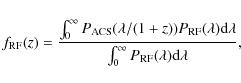 |
(2) |
where
![\begin{figure}
\par\includegraphics[width=8cm,clip]{1923fg2.eps}
\end{figure}](/articles/aa/full_html/2009/26/aa11923-09/img77.png) |
Figure 2:
Function fB(z) for the four ACS filters: B435
(black dashed curve), V606 (black dotted curve), i775 (black dot-dashed curve), and z850
(black solid curve). The grey solid curve is the function fU(z) for
the z850
filter. The vertical black solid line is the maximum redshift,
|
| Open with DEXTER | |
Note that, because the ML method used in the merger fraction determination
(Sect. 4) takes into account the experimental errors, we had to include
in the samples not only the sources with
![]() ,
where
,
where
![]() is
the upper redshift in our study, but also sources with
is
the upper redshift in our study, but also sources with
![]() in order to ensure completeness. Because of this,
in order to ensure completeness. Because of this,
![]() must fulfil the
condition
must fulfil the
condition
![]() ,
which yields
,
which yields
![]() .
We took as minimum redshift in our study
.
We took as minimum redshift in our study
![]() because of the lack of sources at lower redshifts. This yields
because of the lack of sources at lower redshifts. This yields
![]() ,
which ensures completeness and
good statistics. Applying these redshift limits we finally have 1740 galaxies with
,
which ensures completeness and
good statistics. Applying these redshift limits we finally have 1740 galaxies with
![]() and 982 with
and 982 with
![]() .
The
number of galaxies quoted here was obtained after removing problematic
border sources (Sect. 3.1.4).
.
The
number of galaxies quoted here was obtained after removing problematic
border sources (Sect. 3.1.4).
3.1.3 Determining the asymmetry of sources with photometric redshifts
Roughly ![]() % of the sources in our samples do not have spectroscopic
redshifts and we rely on photometric redshift determinations. In these cases, our
source could have its rest-frame B-band flux in two observational ACS filters, within
1
% of the sources in our samples do not have spectroscopic
redshifts and we rely on photometric redshift determinations. In these cases, our
source could have its rest-frame B-band flux in two observational ACS filters, within
1![]() .
To take this into account we assumed three different redshifts for each
photometric source:
.
To take this into account we assumed three different redshifts for each
photometric source:
![]() ,
,
![]() ,
and
,
and
![]() .
We determined the asymmetry in these three redshifts. We then performed a weighted
average of the three asymmetry values such that:
.
We determined the asymmetry in these three redshifts. We then performed a weighted
average of the three asymmetry values such that:
where A(z) is the asymmetry of the source at redshift z. We used the same average procedure with the uncertainties of the three asymmetries and added the result in quadrature to the rms of the three asymmetry values to obtain
3.1.4 Boundary effects and bright source contamination
The signal-to-noise in HST/ACS decreases near the boundaries of the images, where the exposure time is lower. This affects our asymmetry values in two ways: the SExtractor segmentation maps that we use to calculate the asymmetry have many spurious detections, and any of the five backgrounds defined in Sect. 3.1.1 is representative of the noisier source background. The problem with segmentation maps was noticed previously by De Propris et al. (2007), where the segmentation maps for 50% of their initial 129 galaxies with A > 0.35 are incorrect, or are contaminated by bright nearby sources. With this in mind, we visually inspected all the sources looking for boundary or contaminated sources. We found that boundary sources had systematically high asymmetry values, and had segmentation maps contaminated by spurious detections. To avoid biased merger fraction values we excluded all border sources (high and low asymmetric) from the samples. We found only two sources contaminated by bright nearby sources. For these we redefined the SExtractor parameters to construct correct segmentation maps and redetermined the asymmetry.
3.2 Asymmetries at a reference redshift
The asymmetry index measured on survey images systematically varies with the source
redshift due, first, to the (1+z)4 cosmological surface brightness dimming, which
can modify the galaxy area over which asymmetry is measured, and, second, to the loss of
spatial resolution with z. Several papers have attempted to quantify these
effects by degrading the image spatial resolution and flux to simulate the
appearance that a given galaxy would have at different redshifts in a given survey.
Conselice et al. (2003,2008); and Cassata et al. (2005) degraded a few local
galaxies to higher redshifts and found that asymmetries decrease with z.
Conselice et al. (2003) also noted that this decrease depends on image depth,
and that luminous galaxies are less affected. In addition, Conselice et al. (2005)
show that irregular (high asymmetry) galaxies are more affected than ellipticals
(low asymmetry).
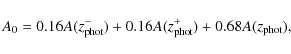
A zeroth-order correction for such biases was implemented by
Conselice et al. (2009,2003,2008) who applied a
![]() term,
defined as the difference between the asymmetry of local galaxies measured in the
original images and the asymmetry of the same galaxies in the images degraded to
redshift z. Their final, corrected asymmetries are
term,
defined as the difference between the asymmetry of local galaxies measured in the
original images and the asymmetry of the same galaxies in the images degraded to
redshift z. Their final, corrected asymmetries are
![]() ,
where A0 is the asymmetry measured in the original images. With these corrections,
all the galaxies have their asymmetry referred to z = 0, and the local merger
criterion
,
where A0 is the asymmetry measured in the original images. With these corrections,
all the galaxies have their asymmetry referred to z = 0, and the local merger
criterion
![]() is then used.
is then used.
In their study, L09 improve on the above procedure, and we apply their methodology
to our data set. We compute a correction term individually for each source in the
catalogue, but rather than attempting to recover z=0 values for A we degrade
each of the galaxy images to redshift
![]() ;
we then obtain our final
asymmetry values
;
we then obtain our final
asymmetry values ![]() directly from the degraded images. With this procedure,
we take into account that each galaxy is affected differently by the degradation;
e.g. the asymmetry of a low luminosity irregular galaxy dramatically decreases with
redshift, while a luminous elliptical is slightly affected. We choose
directly from the degraded images. With this procedure,
we take into account that each galaxy is affected differently by the degradation;
e.g. the asymmetry of a low luminosity irregular galaxy dramatically decreases with
redshift, while a luminous elliptical is slightly affected. We choose
![]() as our reference redshift because a source at this (photometric) redshift
has
as our reference redshift because a source at this (photometric) redshift
has
![]() ;
that is, the probability
that our galaxy belongs to the range of interest is
;
that is, the probability
that our galaxy belongs to the range of interest is ![]() %.
Because we work with asymmetries reduced to
%.
Because we work with asymmetries reduced to
![]() ,
the asymmetry criterion
for mergers,
,
the asymmetry criterion
for mergers, ![]() ,
needs to be reduced to z = 1. We discuss this in Sect. 3.3.
,
needs to be reduced to z = 1. We discuss this in Sect. 3.3.
We have already mentioned that ![]() 60% of the sources in the samples have
spectroscopic redshifts, hence redshift information coming from photometric
redshifts for the remaining
60% of the sources in the samples have
spectroscopic redshifts, hence redshift information coming from photometric
redshifts for the remaining ![]() % of the sources has large uncertainties.
As in the A0 calculation process (Sect. 3.1.3, Eq. (3)),
to take into account the redshift uncertainty when deriving the asymmetries at
% of the sources has large uncertainties.
As in the A0 calculation process (Sect. 3.1.3, Eq. (3)),
to take into account the redshift uncertainty when deriving the asymmetries at
![]() we started from three different initial redshifts for each
source,
we started from three different initial redshifts for each
source,
![]() ,
,
![]() ,
and
,
and
![]() ,
and degraded the
image from these three redshifts to
,
and degraded the
image from these three redshifts to
![]() .
We then performed a weighted
average of the three asymmetry values such that
.
We then performed a weighted
average of the three asymmetry values such that
where A1(z) denotes the asymmetry measured in the image degraded from z to
To obtain the error of the asymmetry, denoted by
![]() ,
for sources with photometric redshifts, we averaged the uncertainties of
the three asymmetries following Eq. (4) and added the result in
quadrature to the rms of the three asymmetry values. The first term
accounts for the signal-to-noise error in the asymmetry value, while the
second term is only important when differences between the three asymmetry
values cannot be explained by the signal-to-noise first term. In sources
with spectroscopic redshifts we took as
,
for sources with photometric redshifts, we averaged the uncertainties of
the three asymmetries following Eq. (4) and added the result in
quadrature to the rms of the three asymmetry values. The first term
accounts for the signal-to-noise error in the asymmetry value, while the
second term is only important when differences between the three asymmetry
values cannot be explained by the signal-to-noise first term. In sources
with spectroscopic redshifts we took as
![]() the uncertainty
of the asymmetry
the uncertainty
of the asymmetry
![]() .
.
The degradation of the images was performed with COSMOSHIFT
(Balcells et al. 2003), which performs repixelation, psf change and flux decrease
over the sky-subtracted source image. The last COSMOSHIFT step is the
addition of a random Poisson sky noise to the degraded source image to mimic the
noise level of the data. As a result of this last step, two COSMOSHIFT
degradations of the same source yield different asymmetry values. We took the
asymmetry of each degraded source, A1(z), to be the median of asymmetry
measurements on five independent degradations of the original source image
from z to
![]() .
With all the aforementioned steps, each A1(z)
determination involved 25 asymmetry calculations, while the uncertainty in
A1(z) was the median of the five individual asymmetry errors.
.
With all the aforementioned steps, each A1(z)
determination involved 25 asymmetry calculations, while the uncertainty in
A1(z) was the median of the five individual asymmetry errors.
The asymmetries ![]() referred to
referred to
![]() provide a homogeneous
asymmetry set that permits consistent morphological studies in the GOODS-S
field (López-Sanjuan et al., in prep.).
provide a homogeneous
asymmetry set that permits consistent morphological studies in the GOODS-S
field (López-Sanjuan et al., in prep.).
3.3 Asymmetry trends with redshift
For a sample of galaxies over a range of redshifts, the statistical change
with z of the measured asymmetries A0 is the combined effect of loss of
information (as shown in the previous section) and changes in the galaxy population.
In contrast, the redshift evolution of ![]() reflects changes in the galaxy
population alone, given that the morphological information in the images used to
determine
reflects changes in the galaxy
population alone, given that the morphological information in the images used to
determine ![]() is homogeneous for the sample. As already discussed in L09
for the Groth field, we show here that the z trends of A0 and
is homogeneous for the sample. As already discussed in L09
for the Groth field, we show here that the z trends of A0 and ![]() are quite different.
are quite different.
In the top panel of Fig. 3 we show the variation of A0 with redshift
in a
![]() selected sample, while in the bottom panel we see the variation
of
selected sample, while in the bottom panel we see the variation
of ![]() for the same sample. In both panels, open squares are the median
asymmetries in
for the same sample. In both panels, open squares are the median
asymmetries in
![]() redshift bins, and the black solid line is the best
linear least-squares fit to the
redshift bins, and the black solid line is the best
linear least-squares fit to the
![]() points. A0 is seen to decrease
with redshift,
A0 = 0.19 - 0.049z, while the
points. A0 is seen to decrease
with redshift,
A0 = 0.19 - 0.049z, while the ![]() distribution is flat,
distribution is flat,
![]() .
For A0, the negative slope reflects the fact that the
loss of information with redshift (negative effect on A) dominates over genuine
population variations (a positive effect because galaxies at higher redshift are
more asymmetric; e.g. Cassata et al. 2005; Conselice et al. 2005).
In
.
For A0, the negative slope reflects the fact that the
loss of information with redshift (negative effect on A) dominates over genuine
population variations (a positive effect because galaxies at higher redshift are
more asymmetric; e.g. Cassata et al. 2005; Conselice et al. 2005).
In ![]() the
information level does not vary with the redshift of the source, so we only see
population effects. In this case the slope is null, but this is a field-to-field
effect: L09, with the same methodology and sample selection, obtain
the
information level does not vary with the redshift of the source, so we only see
population effects. In this case the slope is null, but this is a field-to-field
effect: L09, with the same methodology and sample selection, obtain
![]() .
This indicates that we cannot extrapolate results from one field to another, and that
individual studies of systematics are needed. We take as degradation rate (
.
This indicates that we cannot extrapolate results from one field to another, and that
individual studies of systematics are needed. We take as degradation rate (![]() )
the difference between both slopes and assume that the merger condition
)
the difference between both slopes and assume that the merger condition ![]() varies with redshift as
varies with redshift as
![]() .
.
Is the degradation rate the same for all luminosity selections?
We expect less asymmetry variation with redshift in bright samples,
because they are less affected by cosmological dimming (Conselice 2003).
We repeated the previous analysis with different MB selection cuts,
from
![]() to
to
![]() (the latter is the limiting
magnitude in our study, Sect. 2.2). We summarize the results in
Table 1 and Fig. 4: asymmetry is more affected by
redshift changes in less luminous samples, as expected. Interestingly, the
degradation rate is roughly constant up to MB = -20,
(the latter is the limiting
magnitude in our study, Sect. 2.2). We summarize the results in
Table 1 and Fig. 4: asymmetry is more affected by
redshift changes in less luminous samples, as expected. Interestingly, the
degradation rate is roughly constant up to MB = -20,
![]() (black solid line in Fig. 4), but then becomes
more pronounced by a factor of 2,
(black solid line in Fig. 4), but then becomes
more pronounced by a factor of 2,
![]() ,
in only 0.5 mag.
One could argue that the sharp increase of
,
in only 0.5 mag.
One could argue that the sharp increase of ![]() for
samples including MB > -20 sources arises because such sources have
higher initial asymmetry A0: a faint irregular galaxy is more affected
by loss of information than a bright elliptical. However, we see in the
last column of Table 1 that the mean asymmetry of sources with
z < 1.0 is similar in all samples,
for
samples including MB > -20 sources arises because such sources have
higher initial asymmetry A0: a faint irregular galaxy is more affected
by loss of information than a bright elliptical. However, we see in the
last column of Table 1 that the mean asymmetry of sources with
z < 1.0 is similar in all samples,
![]() .
Hence,
the degradation rate increases because faint sources have lower signal-to-noise
than luminous ones. Because of this, we decided to restrict our study to the
1122 sources with
.
Hence,
the degradation rate increases because faint sources have lower signal-to-noise
than luminous ones. Because of this, we decided to restrict our study to the
1122 sources with
![]() to ensure that degradation affects all the galaxies
in our sample in the same way, making the merger condition
to ensure that degradation affects all the galaxies
in our sample in the same way, making the merger condition
![]() representative.
representative.
![\begin{figure}
\par\includegraphics[width=8cm,clip]{1923fg3a.eps}\par\includegraphics[width=8cm,clip]{1923fg3b.eps}
\end{figure}](/articles/aa/full_html/2009/26/aa11923-09/img113.png) |
Figure 3:
Asymmetry vs. redshift in the
|
| Open with DEXTER | |
Table 1: Degradation rate for different luminosity samples.
![\begin{figure}
\par\includegraphics[width=8cm,clip]{1923fg4.eps}
\end{figure}](/articles/aa/full_html/2009/26/aa11923-09/img121.png) |
Figure 4:
Degradation rate |
| Open with DEXTER | |
![\begin{figure}
\par\includegraphics[width=8cm,clip]{1923fg5.eps}
\end{figure}](/articles/aa/full_html/2009/26/aa11923-09/img122.png) |
Figure 5:
MB distribution of
|
| Open with DEXTER | |
How important is this luminosity dependence for the mass-selected sample?
The MB distribution of
![]() galaxies is
well described by a Gaussian with
galaxies is
well described by a Gaussian with
![]() and
and
![]() ,
Fig. 5. We found that 70% of the galaxies have
,
Fig. 5. We found that 70% of the galaxies have
![]() ,
and
that the degradation rate for the whole sample is
,
and
that the degradation rate for the whole sample is
![]() .
This tells
us that the faint sources in this sample do not significantly affect the
degradation rate, making the
.
This tells
us that the faint sources in this sample do not significantly affect the
degradation rate, making the
![]() merger condition representative
also for the mass-selected sample. In conclusion, we used
merger condition representative
also for the mass-selected sample. In conclusion, we used
![]() for both samples.
for both samples.
4 Merger fraction determination
Following Conselice (2006b), the merger fraction by morphological criteria is
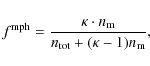
where
Table 2:
Sample characteristics in the
![]() range.
range.
The steps we followed to obtain the merger fraction are described in detail in
LGB08. In this section we provide a short summary. If we define a
two-dimensional histogram in the redshift-asymmetry space and normalize this
histogram to unity, we obtain a two-dimensional probability distribution defined
by the probability of having one source in bin
![]() ,
namely pkl, where the index k spans the redshift bins of size
,
namely pkl, where the index k spans the redshift bins of size ![]() ,
and
the index l spans the asymmetry bins of size
,
and
the index l spans the asymmetry bins of size ![]() .
We consider only two
asymmetry bins split at
.
We consider only two
asymmetry bins split at ![]() ,
such that the probabilities pk1
describe highly distorted galaxies (i.e. merger systems), while the probabilities
pk0 describe normal galaxies. With those definitions, the morphologically based
merger fraction in the redshift interval
[zk, zk+1) becomes
,
such that the probabilities pk1
describe highly distorted galaxies (i.e. merger systems), while the probabilities
pk0 describe normal galaxies. With those definitions, the morphologically based
merger fraction in the redshift interval
[zk, zk+1) becomes
In LGB08 they describe a maximum likelihood (ML) method that yields the most probable values of pkl taking into account not only the z and A values, but also their experimental errors. The method is based on the minimization of the joint likelihood function, which in our case is
![$\displaystyle L(z_{i},A_{i}\vert p^{\prime}_{kl},\sigma_{z_{i}},\sigma_{A_{i}})...
...m_l \frac{{\rm e}^{p'_{kl}}}{4}{\rm ERF}(z,i,k){\rm ERF}(A,i,l)
\bigg\}\biggr],$](/articles/aa/full_html/2009/26/aa11923-09/img145.png)
where
In the above equations,
LGB08 show, using synthetic catalogues, that the experimental errors tend to smooth an initial two-dimensional distribution described by pkl, due to spill-over of sources to neighbouring bins. This leads to a
We obtained the morphological merger fraction by applying
Eq. (9) using the probabilities p'kl recovered by the ML
method. In addition, the ML method provides an estimate of the 68% confidence
intervals of the probabilities p'kl, which we use to obtain the
![]() 68% confidence interval, denoted
[-0pt]
68% confidence interval, denoted
[-0pt]
![]() . This interval is asymmetric because
. This interval is asymmetric because
![]() is described by a log-normal distribution due to the
calculation process (see LGB08 for details). Note that, in LGB08,
is described by a log-normal distribution due to the
calculation process (see LGB08 for details). Note that, in LGB08,
![]() is
used in Eq. (5), but the method is valid for any
is
used in Eq. (5), but the method is valid for any ![]() value.
value.
We also determined the morphological merger fraction by classical counts,
![]() ,
where
,
where
![]() is the number of galaxies in a given bin with
is the number of galaxies in a given bin with
![]() ,
and
,
and
![]() is the total number of
sources in the same bin. We obtained the
is the total number of
sources in the same bin. We obtained the
![]() uncertainties
assuming Poissonian errors in the variables.
uncertainties
assuming Poissonian errors in the variables.
Finally, and following L09, Sect. 4.1, we performed simulations with synthetic catalogues to determine the optimum binning in redshift for which the ML method results are reliable. The simulations were made in the same way as in L09, so here we only report the results of the study: we can define up to three redshift bins, namely z1 = [0.2,0.6), z2 = [0.6,0.85), and z3 = [0.85,1.1). The first bin is wider than the other two, 0.4 vs. 0.25, because of the lower number of sources in the first interval. In the next section we study the merger fraction evolution with redshift with these three bins (Sect. 5.1). We will also provide statistics for the z0 = [0.2,1.1) bin in order to compare the ML and classical merger fraction determinations.
5 Results
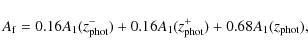
We summarize in Table 2 the main characteristics of
the two samples under study; i.e. the total (
![]() )
and
distorted (
)
and
distorted (![]() )
number of sources, both for classical counts
(
)
number of sources, both for classical counts
(
![]() )
and the ML method (
)
and the ML method (
![]() ), and major merger
fractions. Note that the number of ML method galaxies is not an integer.
Indeed, the ML method gives us a statistical estimate of the probability
), and major merger
fractions. Note that the number of ML method galaxies is not an integer.
Indeed, the ML method gives us a statistical estimate of the probability
![]() of finding one source in the redshift bin k, and
in the asymmetry bin l, so the estimated number of galaxies in that bin,
of finding one source in the redshift bin k, and
in the asymmetry bin l, so the estimated number of galaxies in that bin,
![]() ,
where
,
where
![]() is the total number of galaxies in the sample, need not be an integer.
The merger fraction by the ML method is roughly half that in the classical determination
(0.035 vs. 0.077 in the luminosity-selected sample, 0.025 vs. 0.050 in the
mass-selected sample). This highlights the fact that, whenever the spill-over
effect of large measurement errors is not taken into account, morphological merger
fractions can be overestimated by a factor of
is the total number of galaxies in the sample, need not be an integer.
The merger fraction by the ML method is roughly half that in the classical determination
(0.035 vs. 0.077 in the luminosity-selected sample, 0.025 vs. 0.050 in the
mass-selected sample). This highlights the fact that, whenever the spill-over
effect of large measurement errors is not taken into account, morphological merger
fractions can be overestimated by a factor of ![]() .
We use this result later
in Sect. 6.3, and in the next section we use only merger fractions
obtained by the ML method.
.
We use this result later
in Sect. 6.3, and in the next section we use only merger fractions
obtained by the ML method.
| |
Figure 6:
Asymmetry vs.
|
| Open with DEXTER | |
We find that correction of redshift-dependent biases is equally important. If we use the raw asymmetry values determined on the original images, and apply the local Universe merger selection criterion
A0 > 0.35, the resulting merger fractions come up a factor 2 higher than the ones listed in Table 2. Recall that the latter come from ![]() values homogenised to a common reference
values homogenised to a common reference
![]() (Sect. 3.2). This emphasises that published merger fractions which do not work with redshift-homogeneous data, may be significantly biased. Interestingly, an identical comparison to the one just described, applied to Groth strip data, lead L09 to conclude that redshift effects are not important for merger fraction determinations. The different behaviour of the Groth data from L09 and our GOODS-S data might be due to cosmic variance, or to depth differences between the two data sets. In general though, artificial redshifting of the galaxies is needed to ensure reliable results.
(Sect. 3.2). This emphasises that published merger fractions which do not work with redshift-homogeneous data, may be significantly biased. Interestingly, an identical comparison to the one just described, applied to Groth strip data, lead L09 to conclude that redshift effects are not important for merger fraction determinations. The different behaviour of the Groth data from L09 and our GOODS-S data might be due to cosmic variance, or to depth differences between the two data sets. In general though, artificial redshifting of the galaxies is needed to ensure reliable results.
Table 2 shows that the merger fraction from the mass-selected sample is
lower than that from the luminosity-selected sample. What is the origin of this
difference? To answer this question, we define two subsamples: the faint sample
(galaxies with MB > -20 and
![]() ), and the light-weight sample (sources with
), and the light-weight sample (sources with
![]() and
and
![]() ).
The faint sample comprises 272 sources, while the light-weight sample
comprises 408 sources. In Fig. 6 we show both samples in the mass-asymmetry
plane: light-weight galaxies have higher asymmetry,
).
The faint sample comprises 272 sources, while the light-weight sample
comprises 408 sources. In Fig. 6 we show both samples in the mass-asymmetry
plane: light-weight galaxies have higher asymmetry,
![]() ,
while
faint galaxies are more symmetric,
,
while
faint galaxies are more symmetric,
![]() .
The
light-weight sample comprises 43 sources with
.
The
light-weight sample comprises 43 sources with
![]() (10.5% of the sample),
while the faint sample comprises only seven distorted sources (2.5% of the sample).
These numbers suggest, in agreement with L09, that: (i) an important fraction of the
B-band high asymmetric sources are low-mass disc-disc merger systems that, due to
merger-triggered star-formation, have their B-band luminosity boosted by 1.5 mag
(Bekki & Shioya 2001), enough to fulfil our selection cut
(10.5% of the sample),
while the faint sample comprises only seven distorted sources (2.5% of the sample).
These numbers suggest, in agreement with L09, that: (i) an important fraction of the
B-band high asymmetric sources are low-mass disc-disc merger systems that, due to
merger-triggered star-formation, have their B-band luminosity boosted by 1.5 mag
(Bekki & Shioya 2001), enough to fulfil our selection cut
![]() ;
and (ii) the
faint objects are earlier types dominated by a spheroidal component which, when subject
to a major merger, does not distort enough to be picked up as merger systems by our
asymmetry criterion.
;
and (ii) the
faint objects are earlier types dominated by a spheroidal component which, when subject
to a major merger, does not distort enough to be picked up as merger systems by our
asymmetry criterion.
Table 3:
Morphological major merger fractions
![]() in GOODS-S.
in GOODS-S.
Table 4:
Morphological merger fraction in GOODS-S at
![]() .
.
5.1 Merger fraction evolution
We summarize in Table 3 the morphological merger fraction at different
redshifts in GOODS-S. We obtain low merger fractions, always lower than 0.06,
similar to the L09 results for the Groth field. The merger fraction increases with
redshift in both the luminosity- and the mass-selected samples, but this growth is
more prominent in the mass-selected sample. We can parameterize the merger fraction
evolution as
and fit our data. Note that, in the luminosity-selected sample, we also use the
5.2 Large scale structure effect
It is well known that the more prominent large scale structure (LSS) in the
GOODS-S field is located at redshift z = 0.735 (Ravikumar et al. 2007). In order
to check the effect of this LSS on our derived merger fractions, we recalculated
them by excluding the sources within
![]() of z = 0.735 (Rawat et al. 2008).
In Table 4 we summarize the number of sources in the LSS for each sample
(
of z = 0.735 (Rawat et al. 2008).
In Table 4 we summarize the number of sources in the LSS for each sample
(
![]() ), and the previous and recalculated merger fractions, both in the
field and in the structure. The merger fraction is higher in the LSS than in the
field. Note that the variation in the field values is well reported by the error bars.
How does this LSS affect the previously inferred merger evolution? If we again fit the
data without LSS, we find that
), and the previous and recalculated merger fractions, both in the
field and in the structure. The merger fraction is higher in the LSS than in the
field. Note that the variation in the field values is well reported by the error bars.
How does this LSS affect the previously inferred merger evolution? If we again fit the
data without LSS, we find that
![]() does not change, while the value
of m decreases only by 0.1 in both the luminosity- and the mass-selected samples, so
our conclusions remain the same. We shall therefore use the fit values in Table 3
in the remainder of the paper. We concentrate on the LSS at z = 0.735, and ignore other structures in GOODS-S. The next two more important ones are located at z = 0.66
and z = 1.1. The former is an overdensity in redshift space, but not in the sky plane,
while the latter is a cluster, but comprises an order of magnitude fewer sources than the
z = 0.735 structure (145 vs. 12, Adami et al. 2005).
does not change, while the value
of m decreases only by 0.1 in both the luminosity- and the mass-selected samples, so
our conclusions remain the same. We shall therefore use the fit values in Table 3
in the remainder of the paper. We concentrate on the LSS at z = 0.735, and ignore other structures in GOODS-S. The next two more important ones are located at z = 0.66
and z = 1.1. The former is an overdensity in redshift space, but not in the sky plane,
while the latter is a cluster, but comprises an order of magnitude fewer sources than the
z = 0.735 structure (145 vs. 12, Adami et al. 2005).
6 Discussion
First we compare our results with merger fraction determinations from other authors.
In Fig. 7 we show our results (open squares for
![]() galaxies and
bullets for
galaxies and
bullets for
![]() galaxies). The other points are those
from the literature: the
galaxies). The other points are those
from the literature: the
![]() estimate by L09 of the De Propris et al. (2007)
estimate by L09 of the De Propris et al. (2007)
![]() merger fraction; the merger fraction for B-band luminosity selected
galaxies in AEGIS
merger fraction; the merger fraction for B-band luminosity selected
galaxies in AEGIS![]() (All-Wavelength Extended Groth Strip
International Survey) from Lotz et al. (2008a); the results from Conselice et al. (2009) in
COSMOS
(All-Wavelength Extended Groth Strip
International Survey) from Lotz et al. (2008a); the results from Conselice et al. (2009) in
COSMOS![]() (Cosmological Evolution Survey)
and AEGIS for
(Cosmological Evolution Survey)
and AEGIS for
![]() galaxies; and the merger fraction for
galaxies; and the merger fraction for
![]() galaxies in
GEMS
galaxies in
GEMS![]() (Galaxy Evolution from
Morphology and SEDs) from Jogee et al. (2009). Note that the mass selection from
Jogee et al. (2009) has been adapted to a Salpeter IMF (Salpeter 1955). All the
previous merger fractions except those from Jogee et al. (2009) are from automatic indices for major mergers. The Jogee et al. (2009) results are by visual morphology and reflect
major+minor mergers; the dashed rectangle marks their expected major merger fraction.
For luminosity-selected samples (open symbols) our values are in good agreement with
De Propris et al. (2007), but are lower than those from Lotz et al. (2008a), who apply different
sample selection and merger criteria from ours and do not correct the effect of observational
errors, thus making comparison difficult.
(Galaxy Evolution from
Morphology and SEDs) from Jogee et al. (2009). Note that the mass selection from
Jogee et al. (2009) has been adapted to a Salpeter IMF (Salpeter 1955). All the
previous merger fractions except those from Jogee et al. (2009) are from automatic indices for major mergers. The Jogee et al. (2009) results are by visual morphology and reflect
major+minor mergers; the dashed rectangle marks their expected major merger fraction.
For luminosity-selected samples (open symbols) our values are in good agreement with
De Propris et al. (2007), but are lower than those from Lotz et al. (2008a), who apply different
sample selection and merger criteria from ours and do not correct the effect of observational
errors, thus making comparison difficult.
![\begin{figure}
\par\includegraphics[width=12cm,clip]{1923fg7.eps}
\end{figure}](/articles/aa/full_html/2009/26/aa11923-09/img192.png) |
Figure 7:
Morphological merger fraction vs. redshift for
|
| Open with DEXTER | |
In the mass-selected case our results are in good agreement with the expected
visual major merger fraction from Jogee et al. (2009) (dashed lines), supporting
the robustness of our methodology for obtaining major merger fractions statistically.
Our values are significantly lower that those of Conselice et al. (2009), especially at
![]() ,
where there is a factor 3 difference. The asymmetry calculation performed
by Conselice et al. (2009) does not take into account the spill-over effect of observational errors in their merger fraction
determination. We show here that such effects may lead to the higher value obtained by them.
Conselice et al. (2009) assume two main statistical corrections at
,
where there is a factor 3 difference. The asymmetry calculation performed
by Conselice et al. (2009) does not take into account the spill-over effect of observational errors in their merger fraction
determination. We show here that such effects may lead to the higher value obtained by them.
Conselice et al. (2009) assume two main statistical corrections at
![]() :
the information degradation bias (
:
the information degradation bias (
![]() ,
Sect. 3.2) and the morphological
K-correction (
,
Sect. 3.2) and the morphological
K-correction (
![]() ,
see Conselice et al. 2008, for details). The first correction
is
,
see Conselice et al. 2008, for details). The first correction
is
![]() and has an associated uncertainty of
and has an associated uncertainty of
![]() (Conselice et al. 2003, Table 1). The morphological
K-correction depends on redshift; to simplify the argument, we do not consider its
uncertainty in the following. In addition, each source asymmetry has its own signal-to-noise
uncertainty, which in our study is
(Conselice et al. 2003, Table 1). The morphological
K-correction depends on redshift; to simplify the argument, we do not consider its
uncertainty in the following. In addition, each source asymmetry has its own signal-to-noise
uncertainty, which in our study is
![]() at these redshifts.
We reproduced the same methodology applied by Conselice et al. (2009) on synthetic catalogs created as in Sect. 4. For further details about simulation parameters and assumptions,
see L09. In the simulations we defined two redshift intervals, namely
z2 = [0.6,0.85)
and
z3 = [0.85,1.1), taking our results in these redshift intervals as input merger
fractions,
at these redshifts.
We reproduced the same methodology applied by Conselice et al. (2009) on synthetic catalogs created as in Sect. 4. For further details about simulation parameters and assumptions,
see L09. In the simulations we defined two redshift intervals, namely
z2 = [0.6,0.85)
and
z3 = [0.85,1.1), taking our results in these redshift intervals as input merger
fractions,
![]() in the first interval, and
in the first interval, and
![]() in the second. We then extracted 2000 random sources in the redshift-asymmetry plane,
applying an asymmetry error to them of
in the second. We then extracted 2000 random sources in the redshift-asymmetry plane,
applying an asymmetry error to them of
![]() ,
which is representative of
the asymmetry uncertainties in Conselice et al. (2009). We assumed
,
which is representative of
the asymmetry uncertainties in Conselice et al. (2009). We assumed
![]() for simplicity. Merger fractions were derived from classical histograms as in Conselice et al. (2009). We
repeated this process 100 times and averaged the results. This process yields
for simplicity. Merger fractions were derived from classical histograms as in Conselice et al. (2009). We
repeated this process 100 times and averaged the results. This process yields
![]() in the first interval, and
in the first interval, and
![]() in the second,
which is similar to Conselice et al. (2009) results at these redshifts. In contrast,
the ML method was able to recover the input merger fractions. The exercise demonstrates that the observed differences
betwen the two studies can be naturally explained as a bias introduced in Conselice et al. (2009) by not accounting for spill-over of sources due to observational errors.
The fact that
Conselice et al. (2009) study is performed over
in the second,
which is similar to Conselice et al. (2009) results at these redshifts. In contrast,
the ML method was able to recover the input merger fractions. The exercise demonstrates that the observed differences
betwen the two studies can be naturally explained as a bias introduced in Conselice et al. (2009) by not accounting for spill-over of sources due to observational errors.
The fact that
Conselice et al. (2009) study is performed over
![]() galaxies, 20 times more sources
than in our study, cannot correct the errors. As emphasized by LGB08, experimental systematic errors are not cured by increasing sample size: the ML method is needed.
galaxies, 20 times more sources
than in our study, cannot correct the errors. As emphasized by LGB08, experimental systematic errors are not cured by increasing sample size: the ML method is needed.
6.1 Groth vs. GOODS-S merger fractions: cosmic variance effect
L09 report a morphological merger fraction
 |
(11) |
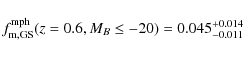
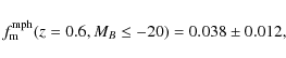
in the Groth field (open diamond in Fig. 7). How does this value compare with the one obtained in GOODS-S? If we use the same selection as in L09, this is,
 |
(12) |
We can see that both values are consistent within their errors. Because both values are determined using the same methodology and sample selection, the difference of
 |
(13) |
where the error is the expected
6.2 Morphological merger fraction evolution in previous studies
In Sect. 5.1 we obtained the values of m and
![]() that describe the morphological merger fraction
evolution in GOODS-S. In this section we compare these values with those in the
literature, where morphological works in B-band selected samples are common.
L09 study the merger fraction for
that describe the morphological merger fraction
evolution in GOODS-S. In this section we compare these values with those in the
literature, where morphological works in B-band selected samples are common.
L09 study the merger fraction for
![]() galaxies in Groth by asymmetries
and taking into account the experimental error bias. Combining their results with
the literature, they obtain
galaxies in Groth by asymmetries
and taking into account the experimental error bias. Combining their results with
the literature, they obtain
![]() ,
consistent to within
,
consistent to within
![]() with our result. Lotz et al. (2008a) study the merger fraction in an
with our result. Lotz et al. (2008a) study the merger fraction in an
![]() selected sample by G and M20 morphological
indices. Their results alone suggest
selected sample by G and M20 morphological
indices. Their results alone suggest
![]() ,
but when combined with
others in the literature they obtain
,
but when combined with
others in the literature they obtain
![]() .
The first case does not
match the local morphological merger fraction by De Propris et al. (2007): with a
similar luminosity cut,
.
The first case does not
match the local morphological merger fraction by De Propris et al. (2007): with a
similar luminosity cut,
![]() ,
and taking into account the different
methodologies (see L09, for details), the merger fractions are very different, 0.006
(De Propris et al. 2007) vs. 0.07 (Lotz et al. 2008a). Because of this, the second m value is
preferred. Kampczyk et al. (2007) study the fraction of visually distorted galaxies in
SDSS
,
and taking into account the different
methodologies (see L09, for details), the merger fractions are very different, 0.006
(De Propris et al. 2007) vs. 0.07 (Lotz et al. 2008a). Because of this, the second m value is
preferred. Kampczyk et al. (2007) study the fraction of visually distorted galaxies in
SDSS![]() (Sloan Digital Sky Survey, local value) and COSMOS
(
(Sloan Digital Sky Survey, local value) and COSMOS
(
![]() value) for
value) for
![]() galaxies. They find that
galaxies. They find that
![]() ,
higher than our value, but consistent to within
,
higher than our value, but consistent to within
![]() .
Finally,
Conselice et al. (2003) study the morphological merger fraction of
.
Finally,
Conselice et al. (2003) study the morphological merger fraction of
![]() by
asymmetries. However, due to the small area of their survey, they have high uncertainties
in the merger fraction at
by
asymmetries. However, due to the small area of their survey, they have high uncertainties
in the merger fraction at
![]() ,
so we do not compare our results with theirs.
In summary, the morphological major merger fraction evolution in MB samples up to
,
so we do not compare our results with theirs.
In summary, the morphological major merger fraction evolution in MB samples up to
![]() is consistent with a
is consistent with a
![]() evolution (weighted average of the
previous m values), although more studies are needed to understand its dependence
on different luminosity selections.
evolution (weighted average of the
previous m values), although more studies are needed to understand its dependence
on different luminosity selections.
The only previous morphological merger fractions in
![]() selected samples are from Conselice et al. (2009,2003,2008). The small
areas in the first two studies (HDF
selected samples are from Conselice et al. (2009,2003,2008). The small
areas in the first two studies (HDF![]() in Conselice et al. 2003; and UDF
in Conselice et al. 2003; and UDF![]() in
Conselice et al. 2008) make their
in
Conselice et al. 2008) make their
![]() values highly undetermined,
and we use their
values highly undetermined,
and we use their
![]() values to constrain the merger fraction evolution at
higher redshifts in Sect. 6.3. Conselice et al. (2009) find
values to constrain the merger fraction evolution at
higher redshifts in Sect. 6.3. Conselice et al. (2009) find
![]() .
This value is lower than ours, but it is higher than typical values in B-band studies,
supporting the hypothesis that merger fraction evolution in mass-selected samples is more
important than in luminosity-selected samples.
.
This value is lower than ours, but it is higher than typical values in B-band studies,
supporting the hypothesis that merger fraction evolution in mass-selected samples is more
important than in luminosity-selected samples.
Other asymmetry studies have used different selection criteria from ours:
Cassata et al. (2005) obtain a merger fraction evolution
![]() in an
in an
![]() selected sample, and combining their results with others in the literature.
Bridge et al. (2007) perform their asymmetry study on a 24
selected sample, and combining their results with others in the literature.
Bridge et al. (2007) perform their asymmetry study on a 24 ![]() m-selected sample (
m-selected sample (
![]() ), finding m = 1.08. However, these values are
difficult to compare with ours because studies with selections in different bands yields
different results (Rawat et al. 2008; Bundy et al. 2004; L09).
), finding m = 1.08. However, these values are
difficult to compare with ours because studies with selections in different bands yields
different results (Rawat et al. 2008; Bundy et al. 2004; L09).
6.3 Merger fraction evolution at higher redshift
Merger fraction studies of
![]() galaxies at
redshift higher than
galaxies at
redshift higher than ![]() are rare. Ryan et al. (2008) address the problem with
pair statistics, while Conselice et al. (2003,2008) use asymmetries. Both
these studies conclude that the merger fraction shows a maximum at
are rare. Ryan et al. (2008) address the problem with
pair statistics, while Conselice et al. (2003,2008) use asymmetries. Both
these studies conclude that the merger fraction shows a maximum at
![]() and decreases at higher z. This tells us that we cannot extrapolate the power-law
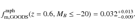
fit (Eq. (10)) to high redshift. Fortunately, Conselice et al. (2008) perform
their study by asymmetries, providing us with a suitably high redshift reference. Note
that, although Conselice et al. (2008) treated the loss of information with redshift, they
do not take into account the overestimation due to the experimental errors. Because the
Conselice et al. (2008) study is performed in UDF, which is located in the GOODS-S area, we
apply a 0.5 factor to the Conselice et al. (2008) merger fractions based on the results of
Sect. 5. In Fig. 8 we show the corrected Conselice et al. (2008)
merger fractions (white dots) and our data (bullets). Note that the
previous power-law fit to our data (black solid line, Sect. 5.1) fails
to explain the merger fraction values at
and decreases at higher z. This tells us that we cannot extrapolate the power-law
fit (Eq. (10)) to high redshift. Fortunately, Conselice et al. (2008) perform
their study by asymmetries, providing us with a suitably high redshift reference. Note
that, although Conselice et al. (2008) treated the loss of information with redshift, they
do not take into account the overestimation due to the experimental errors. Because the
Conselice et al. (2008) study is performed in UDF, which is located in the GOODS-S area, we
apply a 0.5 factor to the Conselice et al. (2008) merger fractions based on the results of
Sect. 5. In Fig. 8 we show the corrected Conselice et al. (2008)
merger fractions (white dots) and our data (bullets). Note that the
previous power-law fit to our data (black solid line, Sect. 5.1) fails
to explain the merger fraction values at
![]() .
.
Following Conselice (2006b), we parameterize the observed tendency as
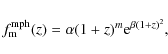
where the local merger fraction is given by
The previous parameterization implies that the merger fraction drops at
![]() ,
being
,
being ![]() at
at ![]() .
On the other hand,
Hopkins et al. (2008) models suggest that the merger fraction of
.
On the other hand,
Hopkins et al. (2008) models suggest that the merger fraction of
![]() galaxies still grows at
galaxies still grows at
![]() ,
being
,
being
![]() at
at ![]() .
In fact, the data in Fig. 8 can also been fitted by
.
In fact, the data in Fig. 8 can also been fitted by
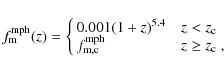
where
![\begin{figure}
\par\includegraphics[width=8cm,clip]{1923fg8.eps}
\end{figure}](/articles/aa/full_html/2009/26/aa11923-09/img249.png) |
Figure 8:
Morphological merger fraction vs. redshift for
|
| Open with DEXTER | |
![\begin{figure}
\par\includegraphics[width=8cm,clip]{1923fg9.eps}
\end{figure}](/articles/aa/full_html/2009/26/aa11923-09/img250.png) |
Figure 9:
Morphological merger rate vs. redshift for
|
| Open with DEXTER | |
Table 5:
Major merger rates
![]() in GOODS-S.
in GOODS-S.
6.4 The major merger rate evolution
We define the major merger rate (
![]() )
as the comoving
number of major mergers per Gyr within a given redshift interval and luminosity
or stellar mass range:
)
as the comoving
number of major mergers per Gyr within a given redshift interval and luminosity
or stellar mass range:
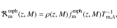 |
(16) |
where
We summarize the merger rates in Table 5 and show these values in
Fig. 9: white symbols are for
![]() galaxies (white
triangle, De Propris et al. 2007; white squares, this work) and bullets for
galaxies (white
triangle, De Propris et al. 2007; white squares, this work) and bullets for
![]() ,
while the grey/black solid line
is the least-squares fit of
,
while the grey/black solid line
is the least-squares fit of
![]() function to the data in the luminosity-/mass-selected sample. The parameters of these fits
are also summarized in Table 5. In spite of the very different merger fraction
evolution, the merger rate evolution of both samples are similar:
function to the data in the luminosity-/mass-selected sample. The parameters of these fits
are also summarized in Table 5. In spite of the very different merger fraction
evolution, the merger rate evolution of both samples are similar:
![]() in the
luminosity sample, while
in the
luminosity sample, while
![]() in the mass sample. As in the merger fraction
case, the results are not affected by the LSS (Sect. 5.2). The reason why the very
different merger fraction evolution tuns into a similar merger rate evolution is the
evolution over cosmic time of the number density of galaxies. The number of
in the mass sample. As in the merger fraction
case, the results are not affected by the LSS (Sect. 5.2). The reason why the very
different merger fraction evolution tuns into a similar merger rate evolution is the
evolution over cosmic time of the number density of galaxies. The number of
![]() galaxies decreases by a factor 3 from z = 1 to z = 0, while
the number of
galaxies decreases by a factor 3 from z = 1 to z = 0, while
the number of
![]() galaxies increases by a factor 3
in the same redshift range.
galaxies increases by a factor 3
in the same redshift range.
We can compare our inferred merger rate with the post-starburst (PSB) rate reported by Wild et al. (2009). The light of PSB galaxies is dominated by A/F stars. Such galaxies are identifiable by their strong Balmer absorption lines compared to their mean stellar age as measured by their 4000 Å break strength. PSB spectra indicate that the formation of O- and early B-type stars has suddenly ceased in the galaxy. The simulations performed by Johansson et al. (2008) find that the PSB phase can only be reached by disc-disc major merger remnants, so the PSB rate and our merger rate may be similar if an evolutionary path connects both populations. The PSB rate, in the range
0.5 < z < 1 and for
![]() galaxies (Salpeter IMF), is
galaxies (Salpeter IMF), is
![]() (1.6-2.9)
(1.6-2.9)
![]() ,
where the interval reflects the uncertainty in the PSB phase time-scale (0.35-0.6 Gyr, Wild et al. 2009). This value compares well with the inferred disc-disc major merger rate at that range,
,
where the interval reflects the uncertainty in the PSB phase time-scale (0.35-0.6 Gyr, Wild et al. 2009). This value compares well with the inferred disc-disc major merger rate at that range,
![]() .
Although the uncertainties in both studies are important, the result suggests that SPB galaxies can be the descendants of our distorted, disc-disc major merger remnants.
.
Although the uncertainties in both studies are important, the result suggests that SPB galaxies can be the descendants of our distorted, disc-disc major merger remnants.
6.4.1 Number density of merger remnants
If we integrate the merger rate over cosmic time, we obtain the number density
of galaxies that have undergone a disc-disc major merger (
![]() )
in a given redshift range:
)
in a given redshift range:
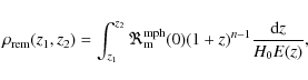
where
Comparing
![]() with the number of
with the number of
![]() galaxies at redshift z1,
galaxies at redshift z1, ![]() ,
we obtain the fraction of merger remnants,
,
we obtain the fraction of merger remnants,
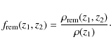
Applying Eq. (18) with the merger rate parameters of the mass sample from Table 5 and the mass functions from Pérez-González et al. (2008), we obtain
The most important error source in our results is the uncertainty in the lower
redshift bin, especially in the mass-selected sample. We repeat our study with a
higher merger fraction in this bin by a factor of two,
![]() ,
and three,
,
and three,
![]() .
With these assumptions
.
With these assumptions
![]() increases to 12% and 18%, respectively. These values remain low,
so our conclusions do not change.
increases to 12% and 18%, respectively. These values remain low,
so our conclusions do not change.
6.4.2 Number of mergers per massive galaxy
As a complement to the previous section we calculate the number of expected disc-disc
major mergers per
![]() galaxy in a given redshift range,
galaxy in a given redshift range,
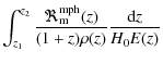
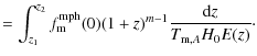
Taking Eq. (14) as the merger fraction parameterization we obtain
These results suggest that most of the disc-disc merger activity of
![]() galaxies happened before
galaxies happened before ![]() ,
this kind of merger being important in galaxy evolution down to this redshift.
It is important to recall that our methodology cannot detect spheroidal major
mergers, so the role of these mergers in the evolution of the red sequence since
,
this kind of merger being important in galaxy evolution down to this redshift.
It is important to recall that our methodology cannot detect spheroidal major
mergers, so the role of these mergers in the evolution of the red sequence since
![]() (Faber et al. 2007; Bell et al. 2004) cannot be addressed by our study. However,
due to the paucity of spheroidal systems at
(Faber et al. 2007; Bell et al. 2004) cannot be addressed by our study. However,
due to the paucity of spheroidal systems at
![]() (Cassata et al. 2005; Conselice et al. 2005),
one expects spheroidal major mergers to be important at lower redshifts;
i.e.
(Cassata et al. 2005; Conselice et al. 2005),
one expects spheroidal major mergers to be important at lower redshifts;
i.e.
![]() .
The simulations of Khochfar & Silk (2008) are in agreement with
this picture: they find that the dry merger rate is two orders of magnitude less than the
wet merger rate at
.
The simulations of Khochfar & Silk (2008) are in agreement with
this picture: they find that the dry merger rate is two orders of magnitude less than the
wet merger rate at
![]() ,
while they are similar at
,
while they are similar at
![]() .
In addition, they
find that the wet merger rate has its maximum at
.
In addition, they
find that the wet merger rate has its maximum at
![]() ,
and then declines by an order
of magnitude until z = 0, a similar evolution to our results,
,
and then declines by an order
of magnitude until z = 0, a similar evolution to our results,
![]() .
To check these
ideas we explore the relative importance of disc-disc mergers in the structural
evolution of
.
To check these
ideas we explore the relative importance of disc-disc mergers in the structural
evolution of
![]() galaxies in a forthcoming paper.
galaxies in a forthcoming paper.
![\begin{figure}
\par\includegraphics[width=8cm,clip]{1923fg10.eps}
\end{figure}](/articles/aa/full_html/2009/26/aa11923-09/img311.png) |
Figure 10:
Comparison between the observed and simulated merger fractions for galaxies with
|
| Open with DEXTER | |
6.5 Comparison with model predictions
The comparison of the predicions by cosmological simulations with our results is not straighforward because we only detect disk-disk (i.e. wet) major mergers, and we select by stellar mass: the simulations from Stewart et al. (2008) point out that the merger fraction depends on merger definition (minor vs. major), selection criteria (halo mass, stellar mass, or luminosity) or the assumed merger time-scale.
The study from Bertone & Conselice (2009) provides predictions for major mergers of
![]() galaxies, assuming a merger time-scale of
galaxies, assuming a merger time-scale of
![]() Gyr. In Fig. 10 we show the predictions (gray solid line), and the observational data from this work (black bullets) and Conselice et al. (2009, crosses). The predictions are in good agreement with our observations, while the Conselice et al. (2009) values are higher than predicted by factors 2 to 6. However, this agreement must be taken as qualitative more than quantitative because (i) cosmological simulations might underestimate the major merger fraction at that stellar mass, as pointed out by Bertone & Conselice (2009), (ii) the predictions are for total (i.e. wet + dry) major mergers, while we report wet major mergers. This can lead in a
Gyr. In Fig. 10 we show the predictions (gray solid line), and the observational data from this work (black bullets) and Conselice et al. (2009, crosses). The predictions are in good agreement with our observations, while the Conselice et al. (2009) values are higher than predicted by factors 2 to 6. However, this agreement must be taken as qualitative more than quantitative because (i) cosmological simulations might underestimate the major merger fraction at that stellar mass, as pointed out by Bertone & Conselice (2009), (ii) the predictions are for total (i.e. wet + dry) major mergers, while we report wet major mergers. This can lead in a ![]() 1% increase in the merger fractions due to dry mergers (Lotz et al. 2008b; Bell et al. 2006a); and, (iii) the GOODS-S merger fractions might be lower that the cosmological value due to cosmic variance (Sect. 6.1). Despite these caveats, the agreement is remarkable.
1% increase in the merger fractions due to dry mergers (Lotz et al. 2008b; Bell et al. 2006a); and, (iii) the GOODS-S merger fractions might be lower that the cosmological value due to cosmic variance (Sect. 6.1). Despite these caveats, the agreement is remarkable.
On the other hand, the simulations of Stewart et al. (2009) provide
![]() for major wet mergers in
for major wet mergers in
![]() galaxies: they predict
galaxies: they predict
![]() -20%, in good agreement with our inferred
-20%, in good agreement with our inferred
![]() %. Finally, Weinzirl et al. (2009) compare their study of
%. Finally, Weinzirl et al. (2009) compare their study of
![]() local spiral galaxies with the predictions by the Khochfar & Silk (2006) and Hopkins et al. (2009b) models. They find that both models are able to explain the observed bulge-to-total ratio (B/T) distribution, and predict that only 13-16% of today's
B/T < 0.75 spirals have undergone a major merger since z = 2. If we assume that all the disc-disc major mergers since z = 2 have enough gas to re-form a disc in the merger remnant (Hopkins et al. 2009a), our
local spiral galaxies with the predictions by the Khochfar & Silk (2006) and Hopkins et al. (2009b) models. They find that both models are able to explain the observed bulge-to-total ratio (B/T) distribution, and predict that only 13-16% of today's
B/T < 0.75 spirals have undergone a major merger since z = 2. If we assume that all the disc-disc major mergers since z = 2 have enough gas to re-form a disc in the merger remnant (Hopkins et al. 2009a), our
![]() % value is an upper limit to the models' predictions, so both are compatible with our results.
% value is an upper limit to the models' predictions, so both are compatible with our results.
7 Conclusions
We have computed the disc-disc major merger fraction and its evolution up to
![]() in the GOODS-S field using morphological criteria. We quantify and
correct for the bias due to varying spatial resolution and image depth with redshift
by artificially redshifting the galaxy images to a common reference redshift of
in the GOODS-S field using morphological criteria. We quantify and
correct for the bias due to varying spatial resolution and image depth with redshift
by artificially redshifting the galaxy images to a common reference redshift of
![]() .
More importantly, we successfully account for the spill-over of sources into
neighbouring bins caused by the errors in asymmetry indices and in
.
More importantly, we successfully account for the spill-over of sources into
neighbouring bins caused by the errors in asymmetry indices and in
![]() ,
through the use of an ML method developed by LGB08. In every case we obtain merger
fractions lower than 0.06, in agreement with the merger fraction determination for
the Groth field (L09). The main improvement
in our study over previous determinations is the robust methodology that takes into
account the signal-to-noise variation of galaxies with z and the observational errors:
previous morphological studies using classical counts overestimate the disc-disc major merger fractions by factors of
,
through the use of an ML method developed by LGB08. In every case we obtain merger
fractions lower than 0.06, in agreement with the merger fraction determination for
the Groth field (L09). The main improvement
in our study over previous determinations is the robust methodology that takes into
account the signal-to-noise variation of galaxies with z and the observational errors:
previous morphological studies using classical counts overestimate the disc-disc major merger fractions by factors of ![]() .
.
The merger fraction evolution in luminosity- and mass-selected
samples are, respectively,
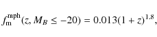 |
(20) |
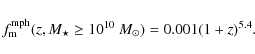 |
(21) |
We study the effect of the LSS on these results and find that merger fractions do not change substantially.
When we compute the merger rate for both samples, the very different merger fraction
evolution becomes a quite similar merger rate evolution:
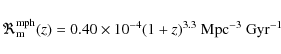 |
(22) |
for
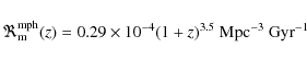 |
(23) |
for
The previous merger rates imply that only ![]() % of today's
% of today's
![]() galaxies have undergone a disc-disc major merger since
galaxies have undergone a disc-disc major merger since ![]() .
Interestingly,
.
Interestingly, ![]() % of
these galaxies at
% of
these galaxies at ![]() have undergone a disc-disc major merger since
have undergone a disc-disc major merger since ![]() ,
which
is compatible with the fraction of bulge-dominated galaxies (E/S0/Sa) at
,
which
is compatible with the fraction of bulge-dominated galaxies (E/S0/Sa) at ![]() (López-Sanjuan et al., in prep.). This suggests that disc-disc major mergers are not
the dominant process in evolution of
(López-Sanjuan et al., in prep.). This suggests that disc-disc major mergers are not
the dominant process in evolution of
![]() galaxies since
galaxies since
![]() ,
with only 0.2 disc-disc major mergers per galaxy, but may be an important
process at z > 1, with
,
with only 0.2 disc-disc major mergers per galaxy, but may be an important
process at z > 1, with ![]() merger per galaxy at 1 < z < 3.
merger per galaxy at 1 < z < 3.
The most important error source in these results is the uncertainty in the lower redshift bin, especially in the mass-selected sample. More studies are needed to improve the statistics at low redshift and avoid cosmic variance effects. Another important issue is the sample definition, given that merger fraction depends on mass and luminosity: larger samples permit us different selection cuts in luminosity and mass, thus improving our knowledge of the importance of disc-disc major mergers in galaxy evolution.
Acknowledgements
We dedicate this paper to the memory of our six IAC colleagues and friends who met with a fatal accident in Piedra de los Cochinos, Tenerife, in February 2007, with particular thanks to Maurizio Panniello, whose teaching of python was so important for this paper. We thank the anonymous referee for suggestions that improved the paper. This work was supported by the Spanish Programa Nacional de Astronomía y Astrofísica through project number AYA2006-12955, AYA2006-02358 and AYA 2006-15698-C02-02. This work was partially funded by the Spanish MEC under the Consolider-Ingenio 2010 Program grant CSD2006-00070: first Science with the GTC (http://www.iac.es/consolider-ingenio-gtc/). This work is based on HST/ACS images from GOODS HST Treasury Program, which is supported by NASA throught grants HST-GO-09425.01-A and HST-GO-09583.01, and in part on observations made with the Spitzer Space Telescope, which is operated by the Jet Propulsion Laboratory, Caltech under NASA contract 1407. P.G.P.G. acknowledges support from the Ramón y Cajal Program financed by the Spanish Government and the European Union.
References
- Abraham, R. G., van den Bergh, S., Glazebrook, K., et al. 1996, ApJS, 107, 1 [NASA ADS] [CrossRef]
- Adami, C., Mazure, A., Ilbert, O., et al. 2005, A&A, 443, 805 [NASA ADS] [CrossRef] [EDP Sciences] (In the text)
- Arnouts, S., Walcher, C. J., Le Fèvre, O., et al. 2007, A&A, 476, 137 [NASA ADS] [CrossRef] [EDP Sciences]
- Balcells, M., Cristóbal-Hornillos, D., & Eliche-Moral, C. 2003, Rev. Mex. Astron. Astrofis. Conf. Ser., 16, 259 [NASA ADS] (In the text)
- Baldry, I. K., Glazebrook, K., Brinkmann, J., et al. 2004, ApJ, 600, 681 [NASA ADS] [CrossRef]
- Bekki, K., & Shioya, Y. 2001, ApJS, 134, 241 [NASA ADS] [CrossRef] (In the text)
- Bell, E. F., Wolf, C., Meisenheimer, K., et al. 2004, ApJ, 608, 752 [NASA ADS] [CrossRef] (In the text)
- Bell, E. F., Naab, T., McIntosh, D. H., et al. 2006a, ApJ, 640, 241 [NASA ADS] [CrossRef]
- Bell, E. F., Phleps, S., Somerville, R. S., et al. 2006b, ApJ, 652, 270 [NASA ADS] [CrossRef]
- Berrier, J. C., Bullock, J. S., Barton, E. J., et al. 2006, ApJ, 652, 56 [NASA ADS] [CrossRef]
- Bertone, S., & Conselice, C. J. 2009, ArXiv e-prints (In the text)
- Bluck, A. F. L., Conselice, C. J., Bouwens, R. J., et al. 2009, MNRAS, 394, L51 [NASA ADS] [CrossRef]
- Bower, R. G., Benson, A. J., Malbon, R., et al. 2006, MNRAS, 370, 645 [NASA ADS]
- Bridge, C. R., Appleton, P. N., Conselice, C. J., et al. 2007, ApJ, 659, 931 [NASA ADS] [CrossRef]
- Bundy, K., Fukugita, M., Ellis, R. S., Kodama, T., & Conselice, C. J. 2004, ApJ, 601, L123 [NASA ADS] [CrossRef]
- Bundy, K., Ellis, R. S., Conselice, C. J., et al. 2006, ApJ, 651, 120 [NASA ADS] [CrossRef]
- Bundy, K., Fukugita, M., Ellis, R. S., et al. 2009, ApJ, 697, 1369 [NASA ADS] [CrossRef]
- Carlberg, R. G. 1990, ApJ, 350, 505 [NASA ADS] [CrossRef] (In the text)
- Cassata, P., Cimatti, A., Franceschini, A., et al. 2005, MNRAS, 357, 903 [NASA ADS] [CrossRef]
- Cassata, P., Cimatti, A., Kurk, J., et al. 2008, A&A, 483, L39 [NASA ADS] [CrossRef] [EDP Sciences]
- Cirasuolo, M., McLure, R. J., Dunlop, J. S., et al. 2007, MNRAS, 380, 585 [NASA ADS] [CrossRef]
- Conselice, C. J. 2003, ApJS, 147, 1 [NASA ADS] [CrossRef] (In the text)
- Conselice, C. J. 2006a, MNRAS, 373, 1389 [NASA ADS] [CrossRef] (In the text)
- Conselice, C. J.2006b, ApJ, 638, 686 (In the text)
- Conselice, C. J., Bershady, M. A., & Jangren, A. 2000, ApJ, 529, 886 [NASA ADS] [CrossRef]
- Conselice, C. J., Bershady, M. A., Dickinson, M., & Papovich, C. 2003, AJ, 126, 1183 [NASA ADS] [CrossRef]
- Conselice, C. J., Blackburne, J. A., & Papovich, C. 2005, ApJ, 620, 564 [NASA ADS] [CrossRef]
- Conselice, C. J., Rajgor, S., & Myers, R. 2008, MNRAS, 386, 909 [NASA ADS] [CrossRef]
- Conselice, C. J., Yang, C., & Bluck, A. F. L. 2009, MNRAS, 361
- Cowie, L. L., Songaila, A., Hu, E. M., & Cohen, J. G. 1996, AJ, 112, 839 [NASA ADS] [CrossRef] (In the text)
- De Lucia, G., & Blaizot, J. 2007, MNRAS, 375, 2 [NASA ADS] [CrossRef]
- De Propris, R., Liske, J., Driver, S. P., Allen, P. D., & Cross, N. J. G. 2005, AJ, 130, 1516 [NASA ADS] [CrossRef]
- De Propris, R., Conselice, C. J., Liske, J., et al. 2007, ApJ, 666, 212 [NASA ADS] [CrossRef]
- Faber, S. M., Willmer, C. N. A., Wolf, C., et al. 2007, ApJ, 665, 265 [NASA ADS] [CrossRef] (In the text)
- Fakhouri, O., & Ma, C.-P. 2008, MNRAS, 386, 577 [NASA ADS] [CrossRef]
- Fontana, A., Salimbeni, S., Grazian, A., et al. 2006, A&A, 459, 745 [NASA ADS] [CrossRef] [EDP Sciences] (In the text)
- Giallongo, E., Salimbeni, S., Menci, N., et al. 2005, ApJ, 622, 116 [NASA ADS] [CrossRef]
- Giavalisco, M., Ferguson, H. C., Koekemoer, A. M., et al. 2004, ApJ, 600, L93 [NASA ADS] [CrossRef] (In the text)
- Gottlöber, S., Klypin, A., & Kravtsov, A. V. 2001, ApJ, 546, 223 [NASA ADS] [CrossRef]
- Governato, F., Gardner, J. P., Stadel, J., Quinn, T., & Lake, G. 1999, AJ, 117, 1651 [NASA ADS] [CrossRef]
- Hopkins, P. F., Hernquist, L., Cox, T. J., & Keres, D. 2008, ApJS, 175, 356 [NASA ADS] [CrossRef] (In the text)
- Hopkins, P. F., Cox, T. J., Younger, J. D., & Hernquist, L. 2009a, ApJ, 691, 1168 [NASA ADS] [CrossRef] (In the text)
- Hopkins, P. F., Somerville, R. S., Cox, T. J., et al. 2009b, ArXiv e-prints
- Hsieh, B. C., Yee, H. K. C., Lin, H., Gladders, M. D., & Gilbank, D. G. 2008, ApJ, 683, 33 [NASA ADS] [CrossRef]
- Jogee, S., Miller, S. H., Penner, K., et al. 2009, ApJ, 697, 1971 [NASA ADS] [CrossRef]
- Johansson, P. H., Naab, T., & Burkert, A. 2008, Astron. Nachr., 329, 956 [NASA ADS] [CrossRef] (In the text)
- Kampczyk, P., Lilly, S. J., Carollo, C. M., et al. 2007, ApJS, 172, 329 [NASA ADS] [CrossRef]
- Kartaltepe, J. S., Sanders, D. B., Scoville, N. Z., et al. 2007, ApJS, 172, 320 [NASA ADS] [CrossRef]
- Khochfar, S., & Burkert, A. 2001, ApJ, 561, 517 [NASA ADS] [CrossRef] (In the text)
- Khochfar, S., & Silk, J. 2006, ApJ, 648, L21 [NASA ADS] [CrossRef] (In the text)
- Khochfar, S., & Silk, J. 2008, ArXiv e-prints (In the text)
- Kolatt, T. S., Bullock, J. S., Somerville, R. S., et al. 1999, ApJ, 523, L109 [NASA ADS] [CrossRef]
- Kriek, M., van der Wel, A., van Dokkum, P. G., Franx, M., & Illingworth, G. D. 2008, ApJ, 682, 896 [NASA ADS] [CrossRef] (In the text)
- Kuchinski, L. E., Freedman, W. L., Madore, B. F., et al. 2000, ApJS, 131, 441 [NASA ADS] [CrossRef]
- Lauger, S., Burgarella, D., & Buat, V. 2005, A&A, 434, 77 [NASA ADS] [CrossRef] [EDP Sciences]
- Lavery, R. J., Remijan, A., Charmandaris, V., Hayes, R. D., & Ring, A. A. 2004, ApJ, 612, 679 [NASA ADS] [CrossRef]
- Le Fèvre, O., Abraham, R., Lilly, S. J., et al. 2000, MNRAS, 311, 565 [NASA ADS] [CrossRef]
- Lin, L., Koo, D. C., Willmer, C. N. A., et al. 2004, ApJ, 617, L9 [NASA ADS] [CrossRef]
- Lin, L., Patton, D. R., Koo, D. C., et al. 2008, ApJ, 681, 232 [NASA ADS] [CrossRef]
- López-Sanjuan, C., García-Dabó, C. E., & Balcells, M. 2008, PASP, 120, 571 [NASA ADS] [CrossRef] (In the text)
- López-Sanjuan, C., Balcells, M., García-Dabó, C. E., et al. 2009, ApJ, 694, 643 [NASA ADS] [CrossRef] (In the text)
- Lotz, J. M., Davis, M., Faber, S. M., et al. 2008a, ApJ, 672, 177 [NASA ADS] [CrossRef]
- Lotz, J. M., Jonsson, P., Cox, T. J., & Primack, J. R. 2008b, MNRAS, 391, 1137 [NASA ADS] [CrossRef] (In the text)
- Masjedi, M., Hogg, D. W., Cool, R. J., et al. 2006, ApJ, 644, 54 [NASA ADS] [CrossRef]
- Miller, S. H., Jogee, S., Conselice, C., et al. 2008, in New Horizons in Astronomy, ed. A. Frebel, J. R. Maund, J. Shen, & M. H. Siegel, ASP Conf. Ser., 393, 235
- Oyaizu, H., Lima, M., Cunha, C. E., Lin, H., & Frieman, J. 2008, ApJ, 689, 709 [NASA ADS] [CrossRef] (In the text)
- Papovich, C., Moustakas, L. A., Dickinson, M., et al. 2006, ApJ, 640, 92 [NASA ADS] [CrossRef] (In the text)
- Patton, D. R., & Atfield, J. E. 2008, ApJ, 685, 235 [NASA ADS] [CrossRef]
- Patton, D. R., Carlberg, R. G., Marzke, R. O., et al. 2000, ApJ, 536, 153 [NASA ADS] [CrossRef]
- Patton, D. R., Pritchet, C. J., Carlberg, R. G., et al. 2002, ApJ, 565, 208 [NASA ADS] [CrossRef]
- Pérez-González, P. G., Rieke, G. H., Egami, E., et al. 2005, ApJ, 630, 82 [NASA ADS] [CrossRef] (In the text)
- Pérez-González, P. G., Rieke, G. H., Villar, V., et al. 2008, ApJ, 675, 234 [NASA ADS] [CrossRef]
- Ravikumar, C. D., Puech, M., Flores, H., et al. 2007, A&A, 465, 1099 [NASA ADS] [CrossRef] [EDP Sciences] (In the text)
- Rawat, A., Hammer, F., Kembhavi, A. K., & Flores, H. 2008, ApJ, 681, 1089 [NASA ADS] [CrossRef] (In the text)
- Ryan, Jr., R. E., Cohen, S. H., Windhorst, R. A., & Silk, J. 2008, ApJ, 678, 751 [NASA ADS] [CrossRef] (In the text)
- Salpeter, E. E. 1955, ApJ, 121, 161 [NASA ADS] [CrossRef] (In the text)
- Scarlata, C., Carollo, C. M., Lilly, S. J., et al. 2007, ApJS, 172, 494 [NASA ADS] [CrossRef]
- Somerville, R. S., Lee, K., Ferguson, H. C., et al. 2004, ApJ, 600, L171 [NASA ADS] [CrossRef] (In the text)
- Stewart, K. R., Bullock, J. S., Barton, E. J., & Wechsler, R. H. 2008, ArXiv e-prints
- Stewart, K. R., Bullock, J. S., Wechsler, R. H., & Maller, A. H. 2009, ArXiv e-prints
- Strateva, I., Ivezic, Z., Knapp, G. R., et al. 2001, AJ, 122, 1861 [NASA ADS] [CrossRef]
- Taylor-Mager, V. A., Conselice, C. J., Windhorst, R. A., & Jansen, R. A. 2007, ApJ, 659, 162 [NASA ADS] [CrossRef]
- Weinzirl, T., Jogee, S., Khochfar, S., Burkert, A., & Kormendy, J. 2009, ApJ, 696, 411 [NASA ADS] [CrossRef] (In the text)
- Wild, V., Walcher, C. J., Johansson, P. H., et al. 2009, MNRAS, 395, 144 [NASA ADS] [CrossRef] (In the text)
Footnotes
- ... catalogues
![[*]](/icons/foot_motif.png)
- http://archive.stsci.edu/prepds/goods/
- ...
MGC
- www.eso.org/~jliske/mgc
- ... AEGIS
- http://aegis.ucolick.org/
- ...
COSMOS
- http://cosmos.astro.caltech.edu/index.html
- ...
GEMS
- http://www.mpia.de/GEMS/gems.htm
- ...
SDSS
- http://www.sdss.org/
- ... (HDF
- http://www.stsci.edu/ftp/science/hdf/hdf.html
- ... UDF
- http://www.stsci.edu/hst/udf
- ...Bluck et al. (2009)
- We apply Eq. (19)
to their best power-law fit of the merger fraction and assume, as previously, that
 Gyr.
Gyr.
All Tables
Table 1: Degradation rate for different luminosity samples.
Table 2:
Sample characteristics in the
![]() range.
range.
Table 3:
Morphological major merger fractions
![]() in GOODS-S.
in GOODS-S.
Table 4:
Morphological merger fraction in GOODS-S at
![]() .
.
Table 5:
Major merger rates
![]() in GOODS-S.
in GOODS-S.
All Figures
| |
Figure 1:
Top: distribution of MB vs. redshift for IRAC catalogue sources.
The black dots are the limiting magnitude of the survey at each redshift, defined
as the third quartile in magnitude distributions. The solid black curve is the best
fit of the limiting magnitude points by a third-degree polynomial. The black dashed
line shows the
MB = -19.5 limit of our study. Bottom: distribution of
|
| Open with DEXTER | |
| In the text | |
| |
Figure 2:
Function fB(z) for the four ACS filters: B435
(black dashed curve), V606 (black dotted curve), i775 (black dot-dashed curve), and z850
(black solid curve). The grey solid curve is the function fU(z) for
the z850
filter. The vertical black solid line is the maximum redshift,
|
| Open with DEXTER | |
| In the text | |
| |
Figure 3:
Asymmetry vs. redshift in the
|
| Open with DEXTER | |
| In the text | |
| |
Figure 4:
Degradation rate |
| Open with DEXTER | |
| In the text | |
| |
Figure 5:
MB distribution of
|
| Open with DEXTER | |
| In the text | |
| |
Figure 6:
Asymmetry vs.
|
| Open with DEXTER | |
| In the text | |
| |
Figure 7:
Morphological merger fraction vs. redshift for
|
| Open with DEXTER | |
| In the text | |
| |
Figure 8:
Morphological merger fraction vs. redshift for
|
| Open with DEXTER | |
| In the text | |
| |
Figure 9:
Morphological merger rate vs. redshift for
|
| Open with DEXTER | |
| In the text | |
| |
Figure 10:
Comparison between the observed and simulated merger fractions for galaxies with
|
| Open with DEXTER | |
| In the text | |
Copyright ESO 2009
Current usage metrics show cumulative count of Article Views (full-text article views including HTML views, PDF and ePub downloads, according to the available data) and Abstracts Views on Vision4Press platform.
Data correspond to usage on the plateform after 2015. The current usage metrics is available 48-96 hours after online publication and is updated daily on week days.
Initial download of the metrics may take a while.