Periodic variation in the water production of comet C/2001 Q4 (NEAT) observed with the Odin satellite

N. Biver; D. Bockelée-Morvan; P. Colom; J. Crovisier; A. Lecacheux; U. Frisk; Å. Hjalmarson; M. Olberg; Aa. Sandqvist

doi:10.1051/0004-6361/200911790

Home

All issues

Volume 501 / No 1 (July I 2009)

A&A, 501 1 (2009) 359-366

Full HTML

Free Access

Issue		A&A Volume 501, Number 1, July I 2009


Page(s)		359 - 366
Section		Planets and planetary systems
DOI		https://doi.org/10.1051/0004-6361/200911790
Published online		29 April 2009

Periodic variation in the water production of comet C/2001 Q4 (NEAT) observed with the Odin satellite

N. Biver¹ - D. Bockelée-Morvan¹ - P. Colom¹ - J. Crovisier¹ - A. Lecacheux¹ - U. Frisk² - Å. Hjalmarson³ - M. Olberg³ - Aa. Sandqvist⁴

1 - LESIA, CNRS UMR 8109, Observatoire de Paris, 5 pl. Jules Janssen, 92195 Meudon, France
2 - Swedish Space Corporation, PO Box 4207, 17104 Solna, Sweden
3 - Onsala Space Observatory, 43992 Onsala, Sweden
4 - Stockholm Observatory, SCFAB-AlbaNova, 10691 Stockholm, Sweden

Received 4 February 2009 / Accepted 21 March 2009

Abstract
Context. Comet C/2001 Q4 (NEAT) was extensively studied with the 1.1-m submillimetre telescope of the Odin satellite. The H₂O line at 557 GHz was regularly observed from 6 March to 16 May 2004 and nearly continuously monitored during 3 periods between 26 April and 2 May 2004.
Aims. This last set of data shows periodic variations in the line intensity, and we looked for characterising the long- and short-term behaviour of this comet.
Methods. We used the variance ratio method and $\chi^2$ minimization to find the period of variation in the water production rate and simulations to infer its amplitude at the nucleus surface.
Results. A 40% periodic variation in the water production rate is measured with a period of $0.816\pm0.004$ day ( $19.58\pm0.1$ h). The comet also exhibits a seasonal effect with a mean peak of outgassing around $2.7\times10^{29}$ molec. s^-1 taking place about 18 days before perihelion.

Key words: astrochemistry - comets: general - comets: individual: C/2001 Q4 (NEAT) - radio lines: solar system - submillimetre

1 Introduction

Comets are the most pristine objects of the Solar System. Cometary nuclei formed and remained far from the Sun, and the molecular inventory of their ices is believed to reflect that of the primordial Solar Nebula in the region where they agglomerated. Water is the main constituent of the ices of cometary nuclei (Festou et al. 2004, and references therein). The study of cometary water is thus crucial for cometary science. Measurements of water production rates allow us to determine the relative abundances of cometary volatiles, whose production rates are measured at the same time. The Odin satellite (Nordh et al. 2003; Frisk et al. 2003) was launched on 20 February 2001 on a Sun-synchronous polar orbit. Odin houses a radiometer with a 1.1-m primary mirror and five receivers at 119 GHz, 486-504 GHz, and 541-580 GHz, which are frequencies that are in large part unobservable from the ground. The H₂O (1₁₀-1₀₁) fundamental line of water at 556.936 GHz is one of the strongest cometary lines, but it cannot be observed from the ground. Its observation in comets has been a major observing topic for Odin. Previous observations of this line in comets have been reported in Neufeld et al. (2000), Lecacheux et al. (2003), and Biver et al. (2007a).

C/2001 Q4 (NEAT) is a dynamically new Oort-cloud comet that came to perihelion on 16 May 2004 at 0.96 AU. It was one of the brightest comets of 2004 and it reached a visual magnitude of m₁=3.3 in early May 2004, as reported by amateur astronomers in the International Comet Quarterly. It has been extensively studied from the ground, especially starting in May 2004 since earlier it was a southern object. Odin monitored its outgassing rate in advance of these observing campaigns. This comet was also active enough that three molecular lines, H₂O(1₁₀-1₀₁) at 557 GHz, H₂¹⁸O(1₁₀-1₀₁) at 548 GHz, and NH₃(1₀-0₀) at 572 GHz were detected around perigee (0.34 AU on 7 May), as reported in Biver et al. (2007a). The water line was also mapped on 16 May 2004.

The investigation of the rotation of cometary nuclei has been done in various ways. Samarasinha et al. (2004) summarises the recent results and the interest of determining rotation properties of cometary nuclei. In this paper we focus on the observations of the H₂O 557 GHz line performed in comet C/2001 Q4 (NEAT) from 6 March to 16 May 2004. They reveal periodic variations in the outgassing linked to the nucleus rotation.

2 Observations

Odin orbits the Earth in 1.6 h. Sixty-three orbits were dedicated to this comet, corresponding to about $63\times0.9$ h observations. About 6 of these are not useful since Odin did not achieve a stable tracking of the comet. (It pointed between 1' and 6 $^{\circ}$ off the comet.) One to three receivers aboard Odin were used simultaneously. Three different set-ups were used for the periods 6 March to 13 April [1], 26 April to 2 May [2] and 15-16 May [3]:

The ``555B2'' receiver was tuned to the H₂O line at 556.936 GHz and connected to the accousto-optical spectrometer (AOS) with a resolution of 1.0 MHz (0.54 km s^-1) and sampling of 0.6 MHz all the time. It was also connected to the AC2 autocorrelator, with an effective resolution of 202 kHz, during periods [1] and [3].
The ``549A1'' receiver was also tuned to the H₂O line at 556.936 GHz and connected to the AC1 autocorrelator, with a resolution of 202 kHz, during period [1]. During period [2] it was tuned to the H₂¹⁸O line at 547.676 GHz and connected to the AC2.
The ``572B1'' receiver was tuned to the NH₃ line at 572.498 GHz and connected to the AC1 during period [2].

During period [2] the main water line at 557 GHz was used to monitor the comet activity. It was strong enough (peak antenna temperature $T_{\rm a}^*\approx10$ K in the Rayleigh-Jeans approximation) to be detected above the $5-\sigma$ level on each single 6-s ON+OFF integration. During the 26 April-2 May period, the calibration was especially stable as the system temperature (3105 K) did not vary by more than 0.3%. It was still within 1% of this value during period [1] but about 10% higher during period [3]. We have collected all information on line intensity, Doppler shift, and pointing offset for each observation (integration over one orbit or fractions of orbits when mapping was done) in Table 1.

Table 1: Log of H₂O observations and production rates in comet C/2001 Q4 (NEAT) (average of AC1 and AC2+AOS data until 13 April).

2.1 Pointing accuracy

The precise knowledge of the pointing is always an issue for comet radio observations, because of the particular column density profile of the atmosphere. The Odin beam has an FWHM of 127 $^{\prime\prime}$ at 557 GHz, and its convolution with the comet signal is roughly Gaussian with an FWHM of about 180 $^{\prime\prime}$ , i.e. not much broader. Ephemeris uncertainties mostly affected period [2] observations: the orbit of this new comet was not perfectly known and the observations at the end of April and early May were affected by ephemeris pointing errors of 30-50 $^{\prime\prime}$ due to the inaccuracy of the orbital elements used at the time of the scheduling. Another source of uncertainty is the satellite attitude: the most recent attitude reconstruction takes the thermal deformations of the Odin platform into account but during 5-10 min at the end or begining of each observation, when only one star tracker is available, the uncertainty can go up to 10 to 60 $^{\prime\prime}$ . These data were excluded from Table 1. We have taken the aberration of light along Odin orbit into acount, which amounts to $\pm5$ $^{\prime\prime}$ . Finally the last source of uncertainty comes from the angle between the pointing axis of the antenna and the reference on the satellite platform. We have estimated this angle and its orientation from the comet maps (and regular pointings on Jupiter) and taken into account its rotation (with respect to RA and Declination axis) during the period of our observations (105 $^{\circ}$ between 24 March and 16 May). Offsets in Table 1 include all those contributions and have been updated from Biver et al. (2007a). The residual uncertainty in the pointing is between 2 $^{\prime\prime}$ and 5 $^{\prime\prime}$ .

3 Conversion of line intensities into production rates

Line intensities are converted into production rates (Table 1). A Haser model with symmetric outgassing and constant radial expansion velocity is used to describe the density, as in our previous studies (Biver et al. 1999). The relative population on the rotational energy levels of water is computed throughout the coma taking into account collisional excitation by neutrals at the gas temperature (assumed constant throughout the coma), collisions with electrons, radiative pumping by Solar infrared flux and self absorption using the Sobolev approximation. The modelling and its accuracy are described in detail in Zakharov et al. (2007). Then numerical integration of the radiative transfer is done to convert production rates into line intensities. As explained in Biver et al. (2007b), since we assume steady state outflow, the retrieved production rates are referred to as ``apparent'' production rates ( $Q_{\rm app}$ ). For the modelling, we use the following parameters:

Expansion velocity: $v_{\rm exp} = 0.85\times(r_{\rm h}[{\rm AU}])^{-0.5}$ km s^-1, ( $r_{\rm h}$ , heliocentric distance), consistent with the shape of H₂¹⁸O and H₂O lines observed with Odin, and other molecules observed with ground-based telescopes in early May (Biver et al. 2009).
Gas temperature: $T=70\times(r_{\rm h}[{\rm AU}])^{-1}$ K, i.e. 70 K around perihelion, as measured from the relative intensity of methanol lines observed at the Institut de radioastronomie millimétrique (IRAM) 30-m telescope between 7 and 11 May 2004 (Biver et al. 2009).
Collision rate with electrons: the scaling factor of the electron density, as defined in Biver et al. (1999, 2007a), was chosen to be x_ne=0.2. It is actually constrained by the radial evolution of the H₂O line intensity observed in the map obtained on 16 May (Biver et al. 2007a). This value minimizes the difference between production rates based on the various offset points.

The assumed photo-dissociation rate of water takes solar activity into account. Table 2 provides the values used for each date. Pointing offsets and other geometrical circumstances are considered when computing the ``apparent'' production rates $Q_{\rm app}$ . The conversion of the line intensities into $Q_{\rm app}$ is needed to compare data from different days to take out the variation in the line intensity unrelated to the intrinsic activity of the comet.

4 Observed variations and simulations

Figure 1 shows the most representative sample of the spectra obtained during nearly continuous monitoring of the comet. Since these spectra were taken in similar conditions (Table 1), the variation in the line mostly reflects the variation in comet activity. We can notice a regular increase followed by a decrease in the line intensity from the long (20 h) series shown as the bottom of Fig. 1. A regular increase in the line intensity is also seen 2 days before (more precisely 39 h $=2\times 19.5$ h, upper series) suggesting some periodic variation in the activity of the comet. For this reason we looked for characterising the variation of the outgassing of the comet with time. To characterise the variations in a more quantitative way, we first converted line intensities into ``apparent'' production rates as explained in Sect. 3, and then simulated those ``apparent'' production rate with a periodic variation of the outgassing at the nucleus surface, as done for comet 9P/Tempel 1 in Biver et al. (2007b). For a sinusoidal variation, a phase difference (time delay) is expected between the production rate Q(t) and the ``apparent'' production rate evolution $Q_{\rm app}(t)$ . This is due to the convolution of a time-dependent density distribution with the beam shape of Odin. The amplitude $\Delta{}Q_{\rm app}$ will be smaller than the variation $\Delta{}Q$ of the sinusoid at the nucleus surface, due to beam averaging. Pointing at offset positions will further damp the variation and increase the delay due to the travel time of the molecules. We made a simple simulation with a production rate:

$\begin{displaymath}Q_{\rm H_2O}(t)=25\times\left(1+0.4\sin\left(\frac{2\pi t}{0.8125}\right)\right)\times10^{28}~\mbox{molec.~s$^{-1}$ ~}\!. \end{displaymath}$

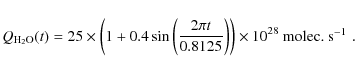(1)

At the nucleus surface, $\Delta{}Q/Q=0.4$ and the period is 0.8125 day (19.5 h), close to what we are to find. The results are given in Table 3: the data between 27 April and 3 May and for the 16 May central point can be analysed together as they show the same damping ( $\Delta{}Q_{\rm app}/\Delta{}Q\approx$ 50%) and delay ( $\approx$ 0.194 day). We do not consider the data at position offsets larger than 2' as they are less sensitive to the periodic variation in the production rate ( $\Delta{}Q_{\rm app}/\Delta{}Q = 8$ -12%, Table 3).

Table 2: Parameters used for the computation of production rates.

In these simulations we did consider the time (and thus radial) variation of the excitation of H₂O due to the varying outgassing rate. Other parameters like the temperature may also vary radially. We tried different $\Delta{}Q/Q$ values (up to 90%), but this does not change the relative ``damping'' factor much or the mean time delay - the apparent production curve gets more asymmetric though.

$\begin{figure} \par\includegraphics[height=18cm, angle=270]{1790fig1.ps} \end{figure}$	Figure 1: Sample of AOS spectra obtained with Odin for comet C/2001 Q4 (NEAT) between 30.10 April and 2.51 May 2004. They are all plotted with the same intensity scale (in the main beam brightness temperature scale) and Doppler velocity scale relative to the nucleus. The upper and lower series are vertically aligned according to the rotation phase.
Open with DEXTER

Table 3: Simulated signal for a periodic variation in the outgassing.

5 Long-term variation of the outgassing

Before looking for periodic variations, it is wise to remove any long-term trend, due to the variation in solar heating ( $1/r_{\rm h}^2$ ) and possible seasonal effects. The mean production rates (daily averages with ranges) are plotted in Fig. 2: the outgassing peaks well before perihelion, so that correcting for a $1/r_{\rm h}^2$ variation is not appropriate. We instead fit the monthly evolution with a Gaussian. In our least square fitting, we put greater weight on the 2 April to 16 May data: for these dates we sampled the full amplitude of the short time variation better and we also mapped the coma several times and thus have a better estimate of the mean production rate. The short March observations, on the other hand, may not provide a good estimate of the mean value around those times. The time component of the fit is $\exp(-(\frac{t-\Delta{}t}{54.0})^2)$ , where t is the time measured in days relative to perihelion and $\Delta{}t=-18$ days is a time shift that can be interpreted as a seasonal effect. It corresponds to an advance of the peak of outgassing with respect to perihelion time. The peak mean outgassing rate is $27\times10^{28}$ molec. s^-1 $\!$ . However, one should be cautious when using these values, since anisotropic outgassing likely influences both the value and time of the peak. It can result in a 10% underestimate of the outgassing rate as explained in Biver et al. (2007a). A Gaussian fit, restricted to the 2 April to 16 May data (Fig. 2), yields

$\begin{displaymath}Q = 27.4\times10^{28}\exp\left(-\left(\frac{t[\rm days]+17.0}{45.7}\right)^2\right) ~\mbox{molec.~s$^{-1}$ ~} \end{displaymath}$

(2)

and is used to remove the long-term trend in the search for short-term variations.

$\begin{figure} \par\resizebox{9cm}{!}{\includegraphics[angle=270]{1790fig2.ps}} \end{figure}$

Figure 2:

Long-term evolution of the water outgassing rate of comet C/2001 Q4 (NEAT). The error-bars for the three first points are based on statistical noise, while for the April-May points they represent the dispersion of the values measured within a day. Two least square fits are plotted: continuous line for $Q\propto\exp(-((t+18)/54)^2)$ ; dashed line: also a Gaussian fit but excluding the March data points (see text).

Open with DEXTER

6 Short-term periodic variations

To search for short-term periodic variations, we selected two subsets: the 26 April to 2 May observations (38 points), plotted in Fig. 3, and the full subset of 57 observations between 2.5 April and 16.1 May (Table 1). We generally excluded data with a pointing offset greater than 70 $^{\prime\prime}$ . The first restricted dataset (a sample of spectra is shown in Fig. 1) has the best consistency: all observations were done in the same week and with the same set-up. In addition, the offset positions were of 30 $^{\prime\prime}$ to 55 $^{\prime\prime}$ due to ephemeris errors, but all in the same direction of the sky (position angle $340\pm10$ $^{\circ}$ ). As a consequence, if the outgassing variations are connected to a rotating jet, we do not expect a significant phase shift between observations. In addition, the increase in ephemeris angular offset (+70%) was partially compensated by the decrease in geocentric distance (-23%), so we expect a very similar sensitivity to the periodic variations for all observations. We do have the same ``damping'' factor around 50% (Table 3). The precision of the production rates, though, are unlikely to be limited by the statistical noise (Table 1), but rather by the pointing accuracy (Sect. 2.1). A 3-4 $^{\prime\prime}$ pointing variation typically results in a 5% uncertainty on the derived production rate for most measurements, to be compared with a typical 1.3% uncertainty due to statistical noise for 45 min integration. This 5% uncertainty has been added quadratically to the rms in Table 1 for all data used in the the $\chi^2$ minimization (e.g., Fig. 3).

$\begin{figure} \par\resizebox{9cm}{!}{\includegraphics[angle=270]{1790fig3.ps}} \end{figure}$	Figure 3: ``Apparent'' water production rates of comet C/2001 Q4 (NEAT) between 26 April and 4 May 2004 and best fit obtained with a sine + harmonic evolution (6 parameters, see text). The time has been corrected for the ``delay'' due to beam averaging and varying geometry.
Open with DEXTER

The other method we used to find a periodicity in the data is the phase dispersion minimization (PDM) method, introduced by Stellingwerf (1978). Particularly useful with a scarce and irregular sampling, it consists in folding the data around a test period Tp, binning the data, and computing the variance ratio between the binned data and the whole sample. This ratio should fluctuate around 1 in the absence of any periodic signal. Should Tp being a significant signal period, then the variance ratio would diminish toward zero, as the local variance would be significantly less than the global one.

The choice of the time origin should not influence the results, hence it is common practice to perform several calculations by time-shifting the folded data and to make an average. The main effect is to smooth the variance ratio curve, which is useful when a small amount of data is available. Considering this small number of data, we limited our number of bins to four, and we performed two time shifts. The result of the PDM method applied to the water production rates is given in Fig. 4. The deepest trough in the curve is at 0.82 day, and we can also see its second sub-harmonic around 1.6 days with a smaller depth, as expected.

We computed the significance level of the variance ratio, which rises when the trough is deeper, according to Stellingwerf (1978). The main parameters are the number of data points, the bin number, and how many time shifts were used. We obtain 98% and 75% for the restricted and the whole sample sets, respectively (see Table 4).

The other method consists in fitting a sine curve (four parameters: average value, amplitude, period Tp, and reference time) or the composite of a sine curve and its harmonic at Tp/2 (6 parameters). The parameters are optimized via $\chi^2$ minimization. For the best fits, we should get a reduced $\chi^2_{\nu}$ close to unity. The $1\sigma$ uncertainty on the fitted period parameter Tp, taken alone, is computed from the extrema of the $\Delta\chi^2=1.0$ envelope.

$\begin{figure} \par\resizebox{9cm}{!}{\includegraphics[angle=270]{1790fig4.ps}}\end{figure}$

Figure 4:

Periodogram analysis of the restricted data set (26 April to 3 May 2004) of comet water production rates. The deepest peak with a variance ratio of 0.5 corresponds to a 0.82 day period. This is the main period found in this analysis: other peaks are mainly coming from harmonics (at 1.6 and 2.4 day) and aliasing. Indeed simulating a pure sine variation of period 0.82 day with the same sampling reproduces all the peaks with variance ratio <0.9.

Open with DEXTER

$\begin{figure} \par\resizebox{9cm}{!}{\includegraphics[angle=270]{1790fig5.ps}} \end{figure}$	Figure 5: Same data as in Fig. 3, folded over one period of 19.53 h, after long-term amplitude correction and ``delay'' correction as in Fig. 3.
Open with DEXTER

6.1 Analysis of the restricted subset

The result of the search of periodicity with the PDM method is shown in Fig. 4 and yields a significant minimum peak at 0.815 day. We then tried to fit a sine (4 parameters) and sine with one harmonic (6 parameters) function to the data. Figures 3 and 5 show the data and results of the $\chi^2$ minimization. The reduced $\chi^2$ is smaller ( $\chi^2_{32}=1.06$ versus $\chi^2_{34}=1.40$ ) when adding an harmonic and the solution found is

$\begin{eqnarray*}\lefteqn{Q_{\rm app}=27.09+4.45\times\sin\left(2\pi\frac{t+15.7... ...6.1050}{0.8139}\right)\times10^{28} ~\mbox{molec.~s$^{-1}$ ~}\!, \end{eqnarray*}$

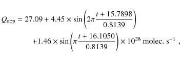
where t is the time in days relative to perihelion, corrected for the delay due to beam dilution. The $\Delta\chi^2=1$ variation yields a $1\sigma$ uncertainty of 0.0032 day ( $\Delta\chi^2=4$ for the $2\sigma$ uncertainty, i.e., a 95.4% confidence level is obtained for the interval Tp=0.8078-0.8208 days). The pure sine solution yields a period of Tp=0.8200 day with a larger uncertainty (Table 4).

6.2 Analysis of the larger subset of 57 points

We also analysed the larger subset with both methods (PDM and sine fitting). The first one gives a peak around Tp=0.817 day (with a nearby less significant peak at 0.852 day) with a 75% confidence level while a sine fit yields Tp=0.8195 day ( $\chi^2_{53}=2.55$ ). The 6-parameter sinusoidal fit yields Tp=0.8188 day ( $\chi^2_{51}=2.39$ , 95.4% confidence level: Tp=0.8177-0.8198 day).

The fit is clearly not as good as for the one week dataset, most likely because the changing geometry (seasonal effect) of the nucleus added some other variation not represented here. Indeed, between 2 April and 16 May the comet moved by 69 $^{\circ}$ around the Sun, and the illumination of the active regions on the nucleus must have changed. The observed seasonal effect ( $\approx$ 18-day shift between perihelion and the peak of activity, Sect. 5) means that the obliquity of the nucleus rotation axis is strong, as suggested by Vasundhara et al. (2007), and that the illumination on active regions changed a lot around perihelion. In particular, the amplitude of rotational variation observed in early April is more than expected. We would have expected a relative amplitude $\Delta{}Q/Q$ twice smaller (Table 3), while instead it is slightly larger. The 1.5-month span is yielding a slightly better precision in estimating the period, although with a lower confidence (Table 4). It is compatible with the period found from the one week dataset.

In summary, we find a clear periodicity in the water outgassing rate, with a best-fit period $Tp=0.816\pm0.004$ day (19h $35\pm6$ min). The observed amplitude of the periodic variation is $\approx$ $5\times10^{28}$ molec. s^-1 for a mean value of $27\times10^{28}$ molec. s^-1 $\!\!$ , i.e. 19%. Given the simulations (Table 3), this implies a real variation in the production rate of $\approx$ $\pm40$ %; e.g. the outgassing rate of the comet at the end of April was varying by a factor greater than 2 in 19.6 h. This must be taken into account when determining mixing ratios from non simultaneous measurements. On the other hand, the analysis of the Doppler shift of the lines does not reveal very significant variations (Table 1): on the restricted subset a sine fit yields a period of $0.70\pm0.01$ day with a reduced $\chi^2_{34} = 2.00$ . But this fit may not be considered as a very good fit since it is barely better than if we fit a straight line ( $\chi^2_{36}=2.66$ ).

Table 4: Time periods found to fit the data.

7 Comparison with other observations

The outgassing of C/2001 Q4 (NEAT) and its variations were the topic of many studies.

On 24-29 April, HST observations of the Lyman- $\alpha$ line gave a mean $Q_{\rm H_2O}$ of $1.9\times10^{29}$ (Weaver et al. 2008), somewhat below the Odin measurements. The OH observations with the Nançay radio telescope began on 2 May, when the comet's declination became higher than -40 $^{\circ}$ (Colom et al. 2004; Crovisier et al. 2009). Production rates $Q_{\rm OH}\approx1.5\times10^{29}$ molec. s^-1 (corresponding to $Q_{\rm H_2O}\approx$ $1.7\times10^{29}$ molec. s^-1 were observed at the beginning of May, somewhat below the values observed by Odin at the same time (Fig. 2). These observations, which consisted of 1-h integrations performed every $\approx$ 24 h, are not suitable for investigating a $\approx$ 20 h periodicity.

Other observers have noticed periodic variation in the activity of this comet. Feldman et al. (2004) find a 17.0 h sine variation with a factor 1.6 from minimum to maximum in the intensity of the CO C-X(0-0) band observed with FUSE on 24 April. Vasundhara et al. (2007), from images obtained between 16 April and 3 June at various places, report a periodic variation of the morphology of the dust coma, but they did not attempt to derive a period. In images obtained at Pic-du-Midi Observatory from 14 to 19 May, Lecacheux & Frappa (2004) find features repeating periodically in the coma of the comet with a $23.2\pm0.25$ h period, close to the determination by Odin.

8 Conclusion

The H₂O outgassing of comet C/2001 Q4 (NEAT) was monitored by the Odin satellite between 6 March and 16 May 2004. The intensity of the 557 GHz H₂O line shows strong variations tracing the non-constant activity of the comet. The following results were obtained:

1.: The outgassing peaked $\approx$ 18 days before perihelion, tracing a seasonal effect, with a mean peak of $27\times10^{28}$ molec. s^-1 $\!$ .
2.: The comet exhibited strong periodic variations in its outgassing with a period of $0.816\pm0.004$ days, implying a $\approx$ 40% variation around the mean value.

The rotation periods of cometary nuclei have been measured in various ways (Samarasinha et al. 2004), either from the light curve of bare nuclei (Lamy et al. 2004) or from the periodic variation of their activity. Rotation-induced outgassing variation can stem either from non sphericity of the nucleus or/and from the presence of areas on the nucleus surface with different activity. The rotation is then traced by spiralling dust jets or shells in the coma (e.g. Jorda et al. 1997) or similar features repeating periodically for the gas (e.g. CN ``jets'', Lederer et al. 2009; the Hale-Bopp CO ``jet'', Bockelée-Morvan et al. 2009) or periodic variations in the outgassing rate (e.g. Jehin et al. 2006; Biver et al. 2007b) as seen here. It can also be traced spectroscopically with periodic variation in the lines shift as in Bockelée-Morvan et al. (2009) and Biver et al. (2007b). While the nucleus light curve measures the synodic rotation period, the other methods measure the rotation with respect to the Sun direction - responsible for the activity - i.e. the length of the day of the comet. Here we find that a large fraction of the gas (40% on average) comes from a source active only during a fraction of the rotation of the nucleus (probably when illuminated by the Sun).

Acknowledgements

Generous financial support from the research councils and space agencies in Canada, Finland, France, and Sweden is gratefully acknowledged. The authors thanks the whole Odin team, including the engineers who have been very supportive of these difficult comet observations. Their help was essential in solving problems in near real time for such time critical observations.

References

Biver, N., Bockelée-Morvan, D., Crovisier, J., et al. 1999, AJ, 118, 1850 [NASA ADS] [CrossRef]
Biver, N., Bockelée-Morvan, D., Crovisier, J., et al. 2007a, Planet. Space Sci., 55, 1058 [NASA ADS] [CrossRef] (In the text)
Biver, N., Bockelée-Morvan, D., Boissier, J., et al. 2007b, Icarus, 191, 494 [NASA ADS] [CrossRef] (In the text)
Biver, N., Bockelée-Morvan, D., Crovisier, J., et al. 2009, in preparation (In the text)
Bockelée-Morvan, D., Henry, F., Biver, N., et al. 2009, A&A, submitted (In the text)
Colom, P., Biver, N., Crovisier, J., Lecacheux, A., & Bockelée-Morvan, D. 2004, in SF2A Scientific Highlights 2004, ed. F. Combes, et al. (EDP Sciences), 69 (In the text)
Crovisier, J., Colom, P., Biver, N., & Bockelée-Morvan, D., 2009 in preparation (In the text)
Feldman, P. D., Weaver, H. A., Christian, D., et al. 2004, BAAS, 36, 1121 [NASA ADS] (In the text)
Festou, M. C., Keller, H. U., & Weaver, H. A. 2004, in Comets II, ed. M. C. Festou, H. U. Keller, & H. A. Weaver (Univ. of Arizona Press), 3 (In the text)
Frisk, U., Hagström, M., Ala-Laurinaho, J., et al. 2003, A&A, 402, L27 [NASA ADS] [CrossRef] [EDP Sciences] (In the text)
Jehin, E., Manfroid, J., Hutsemékers, D., et al. 2006, ApJ, 641, L145 [NASA ADS] [CrossRef] (In the text)
Jorda, L., Rembor, K., Lecacheux, J., et al. 1997, Earth, Moon, and Planets, 77, 167 (In the text)
Lamy, P. L., Toth, I., Fernandez, Y. R., & Weaver, H. A. 2004, in Comets II, ed. M. C. Festou, H. U. Keller, & H. A. Weaver (Univ. of Arizona Press), 223 (In the text)
Lecacheux, J., & Frappa, E. 2004, IAU Circ., 8349 (In the text)
Lecacheux, A., Biver, N., Crovisier, J., et al. 2003, A&A, 402, L55 [NASA ADS] [CrossRef] [EDP Sciences] (In the text)
Lecacheux, J., & Frappa, E. 2004, IAU Circ., 8349 (In the text)
Lederer, S. M., Campins, H., & Osip, D. J. 2009, Icarus, 199, 484 [NASA ADS] [CrossRef] (In the text)
Neufeld, D. A., Stauffer, J. R., Bergin, E. A., et al. 2000, ApJ, 539, L151 [NASA ADS] [CrossRef] (In the text)
Nordh, H. L., von Schéele, F., Frisk, U., et al. 2003, A&A, 402, L21 [NASA ADS] [CrossRef] [EDP Sciences] (In the text)
Samarasinha, N. H., Mueller, B. E. A., Belton, M. J. S., & Jorda, L. 2004, in Comets II, ed. M. C. Festou, H. U. Keller, & H. A. Weaver (Univ. of Arizona Press), 281 (In the text)
Stellingwerf, R. F. 1978, ApJ, 224, 953 [NASA ADS] [CrossRef]
Vasundhara, R., Chakraborty, P., Muneer, S., Masi, G., & Rondi, S. 2007, AJ, 133, 612 [NASA ADS] [CrossRef] (In the text)
Weaver, H. A., A'Hearn, M. F., Arpigny, C., et al. 2008, Asteroids, Comets, Meteors 2008, LPI Contribution, 1405, 8216 (In the text)
Zakharov, V., Bockelée-Morvan, D., Biver, N., Crovisier, J., & Lecacheux, A. 2007, A&A, 473, 303 [NASA ADS] [CrossRef] [EDP Sciences] (In the text)

Footnotes

... satellite: Odin is a Swedish-led satellite project funded jointly by the Swedish National Space Board (SNSB), the Canadian Space Agency (CSA), the National Technology Agency of Finland (Tekes) and the Centre National d'Études Spatiales (CNES, France). The Swedish Space Corporation is the prime contractor, also responsible for Odin operations.
... Quarterly: http://www.cfa.harvard.edu/icq/icq.html

All Tables

Table 1: Log of H₂O observations and production rates in comet C/2001 Q4 (NEAT) (average of AC1 and AC2+AOS data until 13 April).

Table 2: Parameters used for the computation of production rates.

Table 3: Simulated signal for a periodic variation in the outgassing.

Table 4: Time periods found to fit the data.

All Figures

$\begin{figure} \par\includegraphics[height=18cm, angle=270]{1790fig1.ps} \end{figure}$	Figure 1: Sample of AOS spectra obtained with Odin for comet C/2001 Q4 (NEAT) between 30.10 April and 2.51 May 2004. They are all plotted with the same intensity scale (in the main beam brightness temperature scale) and Doppler velocity scale relative to the nucleus. The upper and lower series are vertically aligned according to the rotation phase.
Open with DEXTER
In the text

$\begin{figure} \par\resizebox{9cm}{!}{\includegraphics[angle=270]{1790fig2.ps}} \end{figure}$	Figure 2: Long-term evolution of the water outgassing rate of comet C/2001 Q4 (NEAT). The error-bars for the three first points are based on statistical noise, while for the April-May points they represent the dispersion of the values measured within a day. Two least square fits are plotted: continuous line for $Q\propto\exp(-((t+18)/54)^2)$ ; dashed line: also a Gaussian fit but excluding the March data points (see text).
Open with DEXTER
In the text

$\begin{figure} \par\resizebox{9cm}{!}{\includegraphics[angle=270]{1790fig3.ps}} \end{figure}$	Figure 3: ``Apparent'' water production rates of comet C/2001 Q4 (NEAT) between 26 April and 4 May 2004 and best fit obtained with a sine + harmonic evolution (6 parameters, see text). The time has been corrected for the ``delay'' due to beam averaging and varying geometry.
Open with DEXTER
In the text

$\begin{figure} \par\resizebox{9cm}{!}{\includegraphics[angle=270]{1790fig4.ps}}\end{figure}$	Figure 4: Periodogram analysis of the restricted data set (26 April to 3 May 2004) of comet water production rates. The deepest peak with a variance ratio of 0.5 corresponds to a 0.82 day period. This is the main period found in this analysis: other peaks are mainly coming from harmonics (at 1.6 and 2.4 day) and aliasing. Indeed simulating a pure sine variation of period 0.82 day with the same sampling reproduces all the peaks with variance ratio <0.9.
Open with DEXTER
In the text

$\begin{figure} \par\resizebox{9cm}{!}{\includegraphics[angle=270]{1790fig5.ps}} \end{figure}$	Figure 5: Same data as in Fig. 3, folded over one period of 19.53 h, after long-term amplitude correction and ``delay'' correction as in Fig. 3.
Open with DEXTER
In the text

Current usage metrics show cumulative count of Article Views (full-text article views including HTML views, PDF and ePub downloads, according to the available data) and Abstracts Views on Vision4Press platform.

Data correspond to usage on the plateform after 2015. The current usage metrics is available 48-96 hours after online publication and is updated daily on week days.

Initial download of the metrics may take a while.