| Issue |
A&A
Volume 501, Number 1, July I 2009
|
|
|---|---|---|
| Page(s) | 335 - 348 | |
| Section | The Sun | |
| DOI | https://doi.org/10.1051/0004-6361/200911696 | |
| Published online | 29 April 2009 | |
The Hanle effect in a random magnetic field
Dependence of the polarization on statistical properties of the magnetic field
H. Frisch1 - L. S. Anusha2,1 - M. Sampoorna2 - K. N. Nagendra2
1 - Université de Nice, Observatoire de la Côte d'Azur, CNRS, Laboratoire Cassiopée, BP 4229, 06304 Nice Cedex 4, France
2 - Indian Institute of Astrophysics, Koramangala, Bangalore 560 034, India
Received 21 January 2009 / Accepted 18 March 2009
Abstract
Context. The Hanle effect is used to determine weak turbulent magnetic fields in the solar atmosphere, usually assuming that the angular distribution is isotropic, the magnetic field strength constant, and that micro-turbulence holds, i.e. that the magnetic field correlation length is much less than a photon mean free path.
Aims. To examine the sensitivity of turbulent magnetic field measurements to these assumptions, we study the dependence of Hanle effect on the magnetic field correlation length, its angular, and strength distributions.
Methods. We introduce a fairly general random magnetic field model characterized by a correlation length and a magnetic field vector distribution. Micro-turbulence is recovered when the correlation length goes to zero and macro-turbulence when it goes to infinity. Radiative transfer equations are established for the calculation of the mean Stokes parameters and they are solved numerically by a polarized approximate lambda iteration method.
Results. We show that optically thin spectral lines and optically very thick ones are insensitive to the correlation length of the magnetic field, while spectral lines with intermediate optical depths (around 10-100) show some sensitivity to this parameter. The result is interpreted in terms of the mean number of scattering events needed to create the surface polarization. It is shown that the single-scattering approximation holds good for thin and thick lines but may fail for lines with intermediate thickness. The dependence of the polarization on the magnetic field vector probability density function (PDF) is examined in the micro-turbulent limit. A few PDFs with different angular and strength distributions, but equal mean value of the magnetic field, are considered. It is found that the polarization is in general quite sensitive to the shape of the magnetic field strength PDF and somewhat to the angular distribution.
Conclusions. The mean field derived from Hanle effect analysis of polarimetric data strongly depends on the choice of the field strength distribution used in the analysis. It is shown that micro-turbulence is in general a safe approximation.
Key words: line: formation - polarization - magnetic fields - radiative transfer
1 Introduction
As pointed out by Stenflo (1982, see also, 1994, 2009), the Hanle effect provides a powerful diagnostic for detecting the presence of a weak turbulent magnetic field. The physical origin of this field and symmetry properties of the observed linear polarization suggest that the field scale of variation is small compared to the mean free path of photons and hence that ``micro-turbulence'' could be assumed. This allows one to replace all the physical parameters depending on the magnetic field by their average over the magnetic field vector PDF (probability density function). All the determinations of solar turbulent magnetic fields have been carried out so far with this approximation (Faurobert et al. 2009; Faurobert-Scholl 1993; Bommier et al. 2005; Trujillo Bueno et al. 2004; Faurobert-Scholl 1996; Faurobert 2001). In addition, it is usually assumed that the magnetic field PDF is isotropically distributed and that its strength has a single value. The Hanle problem reduces then to a resonance polarization problem with a modified polarization parameter that is in general smaller (Stenflo 1994,1982).
In a preceding paper (Frisch 2006, henceforth referred to as HF06), a model magnetic field has been introduced allowing one to examine the possible effects of a finite magnetic field correlation length (comparable to a typical photon mean free path). Equations have been established for calculating the mean Stokes parameters, but no numerical results were given. In the present paper, the equations given in HF06 are rewritten in a form easily amenable to a numerical solution. An iterative method of solution of the ALI type (approximate lambda iteration) is used to calculate the mean Stokes parameters. We examine their dependence on the correlation length of the magnetic field and analyze the results in terms of the mean number of scattering events contributing to the formation of the surface polarization. We also investigate the sensitivity of the mean Stokes parameters to the shape of the magnetic field PDF, the objective being to see whether the Hanle effect can provide some clue to the behavior of this quantity.
In Sect. 2, we describe the magnetic field, the atomic and atmospheric models (they are the same as in HF06). We establish the transfer equations for the calculation of the mean Stokes parameters in Sect. 3. In Sect. 4 we describe an ALI type numerical method of solution. In Sect. 5 we describe different types of PDFs used in our investigation. The finite correlation effects are presented in Sect. 6 and analyzed in Sect. 7. Finally, in Sect. 8, we calculate the mean polarization for various types of magnetic field strength PDFs, in the framework of micro-turbulence. Some technical details about transfer equations and calculations of the mean Stokes parameters are presented in Appendices A and B.
2 Assumptions
We consider a two-level atom with unpolarized ground-level and assume
complete frequency redistribution. The ![]() redistribution
matrix takes the form
redistribution
matrix takes the form
where x' and x are the frequencies of incident and scattered beams measured in Doppler width units from line center and n', n their directions. The function
where
In this paper we consider a
one-dimensional medium (plane-parallel atmosphere). The direction of
the magnetic field and of the radiation beams are reckoned in an
atmospheric reference frame with the z-axis along the outward normal to
the medium. The polar angles of the magnetic field direction are
denoted by
![]() and
and ![]() ,
and the polar angles of the
directions n and n' are denoted by
,
and the polar angles of the
directions n and n' are denoted by ![]() ,
,
![]() and
and
![]() ,
,
![]() (see Fig. 1).
(see Fig. 1).
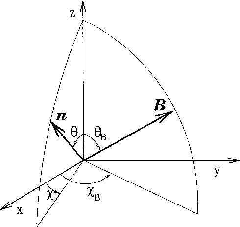 |
Figure 1:
Atmospheric reference frame with the definition of ( |
| Open with DEXTER | |
The random magnetic field B is modeled by a Kubo-Anderson
process (KAP). It is a Markov process, discontinuous, stationary, and
piecewise constant (Brissaud & Frisch 1971, 1974). By definition, a
random function m(t) is a KAP, if the jumping times ti are
uniformly and independently distributed in
![]() according to a Poisson distribution. Furthermore, m(t)=mi for
according to a Poisson distribution. Furthermore, m(t)=mi for
![]() where the mi are independent random variables with
the same probability density P(m). A KAP is thus fully
characterized by a probability density P(m) and a correlation time
where the mi are independent random variables with
the same probability density P(m). A KAP is thus fully
characterized by a probability density P(m) and a correlation time
![]() ,
with
,
with ![]() the density of jumping times on
the time axis (Papoulis 1965, p. 557). For a KAP, the covariance
the density of jumping times on
the time axis (Papoulis 1965, p. 557). For a KAP, the covariance
![]() varies as
varies as
![]() ,
this means
that the spectrum is algebraic.
,
this means
that the spectrum is algebraic.
For the Hanle effect, polarization is created by a scattering process,
which implies that the photons make a random walk inside the
medium. If the magnetic field is a Markov process, say along the
normal to a plane-parallel atmosphere, the radiation field at a point
r, depends on magnetic field values below and above the point
r. To take advantage of the Markov character of the magnetic
field, it is necessary to simplify a little and assume that the
magnetic field is a random process in time, defined by a density
![]() and a probability density P(B). This approach was
first used for random velocities with a finite correlation length by
Frisch & Frisch (1976). Its shortcoming is that it ignores
correlations between photons that return to the same turbulent element
after having been scattered a number of times (Frisch & Frisch 1975). The Stokes
vector I then has to be taken as time dependent.
Standard techniques of solutions for stochastic differential equations
with Markov coefficients become applicable (Brissaud & Frisch 1974). They rely on
the crucial remark that the joint random process
in time
and a probability density P(B). This approach was
first used for random velocities with a finite correlation length by
Frisch & Frisch (1976). Its shortcoming is that it ignores
correlations between photons that return to the same turbulent element
after having been scattered a number of times (Frisch & Frisch 1975). The Stokes
vector I then has to be taken as time dependent.
Standard techniques of solutions for stochastic differential equations
with Markov coefficients become applicable (Brissaud & Frisch 1974). They rely on
the crucial remark that the joint random process
in time
![]() is also a Markov process. To
simplify the notation we have omitted other independent variables on
which the radiation field depends. As shown in HF06, the combination
of the time-dependent transfer equation, with the evolution
equation for the probability density of the joint process
is also a Markov process. To
simplify the notation we have omitted other independent variables on
which the radiation field depends. As shown in HF06, the combination
of the time-dependent transfer equation, with the evolution
equation for the probability density of the joint process
![]() ,
provides a time-dependent transfer equation
for a conditional mean Stokes vector
I(t,r,x,n|B). For this radiation field, B plays the role of an
additional independent variable with values distributed according to
the probability density P(B) (for the definition of the
conditional mean see HF06).
,
provides a time-dependent transfer equation
for a conditional mean Stokes vector
I(t,r,x,n|B). For this radiation field, B plays the role of an
additional independent variable with values distributed according to
the probability density P(B) (for the definition of the
conditional mean see HF06).
The next step is to consider the stationary solution,
I(r,x,n|B), for
![]() .
It satisfies a transfer
equation that has the usual advection, scattering, and primary source
terms, but also contains an additional term describing the action of
the magnetic field. Somewhat similar equations (without the scattering
term) have been introduced for the Zeeman effect by Carroll & Staude (2005). The mean Stokes parameters that one is looking for are given by
.
It satisfies a transfer
equation that has the usual advection, scattering, and primary source
terms, but also contains an additional term describing the action of
the magnetic field. Somewhat similar equations (without the scattering
term) have been introduced for the Zeeman effect by Carroll & Staude (2005). The mean Stokes parameters that one is looking for are given by
In the next section we construct the stationary transfer equation for the conditional mean Stokes vector. We work with the irreducible components of the Stokes vector because they satisfy transfer equations that are simpler than the transfer equations for the Stokes parameters themselves.
3 The transfer problem
We now concentrate on the case of a one-dimensional slab. We
introduce the frequency averaged line optical depth ![]() defined by
defined by
![]() with z the coordinate along the vertical axis (see
Fig. 1) and k(z) the absorption coefficient
per unit length. We denote by T the total optical thickness of the
slab with the surface at
with z the coordinate along the vertical axis (see
Fig. 1) and k(z) the absorption coefficient
per unit length. We denote by T the total optical thickness of the
slab with the surface at ![]() towards the observer. We assume
that the incident radiation is zero on both sides of the slab.
towards the observer. We assume
that the incident radiation is zero on both sides of the slab.
For the deterministic Hanle effect with complete frequency
redistribution, each component
![]() of the
emission term in the transfer equation (sum of the scattering and primary
source terms) has an expansion of the form
of the
emission term in the transfer equation (sum of the scattering and primary
source terms) has an expansion of the form
Starting from this expression, one can show (Frisch 2007, henceforth HF07) that the Stokes parameters have a similar expansion that can be written as
where
3.1 Transfer equation for the conditional mean Stokes parameters
Proceeding as described in Sect. 2 (see also HF06),
we find that
![]() satisfies
the transfer equation
satisfies
the transfer equation

where
with
The operator
The matrix
Averaging Eq. (6) over
P(B), we see that
![]() satisfies the transfer equation
satisfies the transfer equation
![\begin{displaymath}\mu {\partial \langle{\bm{\mathcal I}}\rangle(\tau,x,\mu)\ove...
...le(\tau,x,\mu) - \langle{\bm{\mathcal
S}}\rangle(\tau)\bigr],
\end{displaymath}](/articles/aa/full_html/2009/25/aa11696-09/img81.png)
where
3.2 Integral equation for
 (
( B)
B)
With the boundary condition that there is no incident radiation on the
outer surfaces of the slab, the formal solution of
Eq. (6) can be written as
![$\displaystyle {\bm{\mathcal I}}(\tau,x,\mu\vert{\bm B})=
-\int_0^\tau
\exp\left...
...]\varphi(x){\bm{\mathcal S}}(\tau'\vert~\cdot)~
{{\rm d}\tau'\over\mu};\ \mu<0.$](/articles/aa/full_html/2009/25/aa11696-09/img86.png)
The operator
where
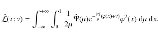
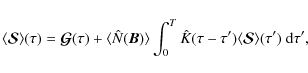
where g(B) is known, one finds a simple expression that is easily expressed in terms of elementary Laplace transforms (for details see HF06; also Frisch & Frisch 1976). We thus obtain


The combination of Eqs. (15) and (16) with Eq. (7) yields the integral equation
![\begin{displaymath}{\bm{\mathcal S}}(\tau\vert{\bm B})= {\bm{\mathcal G}}(\tau) +\hat N(\bm
B)\Lambda[{\bm{\mathcal S}}],
\end{displaymath}](/articles/aa/full_html/2009/25/aa11696-09/img94.png)
where
![$\displaystyle \Lambda[{\bm{\mathcal S}}]= \int_0^T {\rm d}\tau'\Biggl\{\hat {\m...
...\! P({\bm B'}){\bm{\mathcal
S}}(\tau'\vert{\bm B'})~ {\rm d}^3{\bm B'}\Biggr\},$](/articles/aa/full_html/2009/25/aa11696-09/img95.png)
with
For
where
4 A PALI type numerical method of solution
Several numerical methods of solution have been developed to solve
integral equations arising in the study of the Hanle effect with
a deterministic or micro-turbulent magnetic field. In Landi Degl'Innocenti et al. (1990),
the system of linear integral equations
for the components
![]() is transformed into a
system of linear equations for the
is transformed into a
system of linear equations for the
![]() with
with
![]() the optical depth grid points. In this reference, the unknown
functions are actually the density matrix elements
the optical depth grid points. In this reference, the unknown
functions are actually the density matrix elements
![]() ,
but for a two-level atom with complete frequency redistribution,
,
but for a two-level atom with complete frequency redistribution,
![]() and
and
![]() are proportional (see e.g. Landi Degl'Innocenti & Bommier 1994).
are proportional (see e.g. Landi Degl'Innocenti & Bommier 1994).
Iterative methods of the ALI type have
been developed for the Hanle effect with complete frequency
redistribution (Manso Sainz & Trujillo Bueno 2003; Nagendra et al. 1998; Manso Sainz & Trujillo Bueno 1999) and partial frequency
redistribution (Fluri et al. 2003; Sampoorna et al. 2008a; Nagendra et al. 1999). For
partial frequency redistribution, the unknown functions depend on two
independent variables: optical depth and frequency. Here we have a
similar problem, the independent variables being now the optical depth
and the magnetic field vector. We have developed a PALI method (P for
polarized) described below to solve the integral Eq. (17) for
![]() .
The results are presented in Sect. 6.
.
The results are presented in Sect. 6.
We followed a standard approach by which one introduces an
approximate ![]() operator denoted by
operator denoted by
![]() ,
choosing for
,
choosing for
![]() the diagonal of
the diagonal of ![]() with respect to optical
depth. This is the so-called Jacobi scheme (Stoer & Bulirsch 1983). It is
the only one that has been used for partial frequency
redistribution (see e.g. the review by Nagendra & Sampoorna 2009, and
references therein) and seemed to be an appropriate choice
for exploratory work with random magnetic fields. More efficient iteration methods
based on the Gauss-Seidel scheme have been developed for
complete frequency redistribution (see e.g. Léger et al. 2007; Trujillo Bueno & Fabiani Bendicho 1995).
with respect to optical
depth. This is the so-called Jacobi scheme (Stoer & Bulirsch 1983). It is
the only one that has been used for partial frequency
redistribution (see e.g. the review by Nagendra & Sampoorna 2009, and
references therein) and seemed to be an appropriate choice
for exploratory work with random magnetic fields. More efficient iteration methods
based on the Gauss-Seidel scheme have been developed for
complete frequency redistribution (see e.g. Léger et al. 2007; Trujillo Bueno & Fabiani Bendicho 1995).
The Jacobi iteration scheme is
with

and
![\begin{displaymath}{\bm{\mathcal J}}^{(n)}(\tau\vert{\bm B})= \Lambda\left[{\bm{\mathcal S}}^{(n)}\right].
\end{displaymath}](/articles/aa/full_html/2009/25/aa11696-09/img112.png)
The superscript (n) refers to the iteration step, and
The righthand side in Eq. (21) is easy to calculate. Knowing
![]() ,
one can calculate its mean
value
,
one can calculate its mean
value
![]() by averaging over
P(B). Equations (15) and (16)
are then used to calculate
by averaging over
P(B). Equations (15) and (16)
are then used to calculate
![]() .
A short characteristic method (Kunasz & Auer 1988; Auer & Paletou 1994) is used for
this step. Finally
.
A short characteristic method (Kunasz & Auer 1988; Auer & Paletou 1994) is used for
this step. Finally
![]() is deduced from Eq. (8).
is deduced from Eq. (8).
Equation (18) shows that we only need the diagonal operator
corresponding to
![]() ,
henceforth denoted
,
henceforth denoted
![]() ,
to construct the operator
,
to construct the operator
![]() .
As Eq. (19) shows, it can be calculated by a
standard method introduced in Auer & Paletou (1994). At each grid
point in space, we solve a transfer equation, like
Eq. (10), where
.
As Eq. (19) shows, it can be calculated by a
standard method introduced in Auer & Paletou (1994). At each grid
point in space, we solve a transfer equation, like
Eq. (10), where
![]() is replaced by
is replaced by
![]() and the source term replaced by a point source at
the grid point under consideration. A short characteristic method
is also used for this step. Finally, the elements of
and the source term replaced by a point source at
the grid point under consideration. A short characteristic method
is also used for this step. Finally, the elements of
![]() are obtained by performing the integration over
x and
are obtained by performing the integration over
x and ![]() (see Eq. (19)).
(see Eq. (19)).
The corrections
![]() are
solutions of Eq. (21). Since the operator
are
solutions of Eq. (21). Since the operator
![]() is diagonal in space, there is no coupling between the
different depth points. At each depth point
is diagonal in space, there is no coupling between the
different depth points. At each depth point ![]() ,
we have a
system of linear equations for
,
we have a
system of linear equations for
![]() .
The dimension of this system is
.
The dimension of this system is
![]() ,
with NC the number of irreducible components (6
for linear polarization) and NB the number of grid points
needed to describe the magnetic field PDF. Since the magnetic field
is defined by its strength B, inclination
,
with NC the number of irreducible components (6
for linear polarization) and NB the number of grid points
needed to describe the magnetic field PDF. Since the magnetic field
is defined by its strength B, inclination
![]() ,
and azimuth
,
and azimuth
![]() (see Fig. 1),
(see Fig. 1),
![]() ,
with NB,
,
with NB,
![]() ,
and
,
and
![]() the number of grid
points corresponding to the respective variables.
the number of grid
points corresponding to the respective variables.
Table 1: A list of different PDFs used in this paper.
At each depth point ![]() ,
the linear system of equations for the
,
the linear system of equations for the
![]() can be written as
can be written as
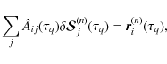
where i and j are indices for the magnetic field vector grid points (
The
The convergence properties of this iteration method are similar to
those of other PALI methods used for polarized problems
(Nagendra et al. 1999,1998). The new feature here is the discretization of
the magnetic field vector. Typically we have been using NB= 40.
For an isotropic angular distribution,
![]() points
in the interval
points
in the interval ![]() ,
the integration over
,
the integration over
![]() being
performed with a Gauss-Legendre quadrature. Significantly higher values of
being
performed with a Gauss-Legendre quadrature. Significantly higher values of
![]() are needed for angular distributions that are
peaked along some direction (see Sect. 5). All the
magnetic field PDFs chosen here have a cylindrical symmetry about the
normal to the atmosphere, so no integration over
are needed for angular distributions that are
peaked along some direction (see Sect. 5). All the
magnetic field PDFs chosen here have a cylindrical symmetry about the
normal to the atmosphere, so no integration over ![]() is
needed. For the integration over
is
needed. For the integration over ![]() ,
we use 5 to 7 points
per decade.
,
we use 5 to 7 points
per decade.
In this work, we consider
self-emitting slabs. The primary source is
![]() with
with ![]() the rate of destruction by
inelastic collisions (see Appendix A) and
the rate of destruction by
inelastic collisions (see Appendix A) and ![]() the Planck function at line center. The line absorption profile
the Planck function at line center. The line absorption profile
![]() is a Voigt function with damping parameter a. The
atomic and atmospheric models are thus defined by a set of parameters
(
is a Voigt function with damping parameter a. The
atomic and atmospheric models are thus defined by a set of parameters
(
![]() )
where a,
)
where a,
![]() and
and ![]() are assumed to be constant with
are assumed to be constant with ![]() .
The solution of the transfer equation is then symmetrical with respect
to T/2.
.
The solution of the transfer equation is then symmetrical with respect
to T/2.
The magnetic kernel elements
NKQQ'(B) are defined in
Appendix A. In all the calculations we assume a
normal Zeeman triplet, an electric-dipole transition and no
depolarizing collisions. For the magnetic field, the parameters are
the magnetic field strength B, the polar angles
![]() and
and ![]() ,
the density
,
the density ![]() of jumping points and the PDF P(B). For the Hanle effect, it is convenient to use the
Hanle efficiency factor
of jumping points and the PDF P(B). For the Hanle effect, it is convenient to use the
Hanle efficiency factor
![]() ,
instead of the magnetic field
strength itself. The definition of
,
instead of the magnetic field
strength itself. The definition of
![]() is recalled in
Appendix A.
is recalled in
Appendix A.
5 A choice of magnetic field vector PDFs
For the quiet Sun, a few PDFs have been proposed in the literature for
field strength B and for inclination
![]() of the
magnetic field with respect to the vertical direction. They are based on
the analysis of magneto-convection simulations, inversion of
Stokes parameters, and heuristic considerations (see
e.g. Sánchez Almeida 2007; Sampoorna et al. 2008b; Dominguez Cerdena et al. 2006; Trujillo Bueno et al. 2004). Almost nothing is
known about the azimuthal distribution. For our investigation we have chosen PDFs
that are cylindrically symmetrical and have the form
of the
magnetic field with respect to the vertical direction. They are based on
the analysis of magneto-convection simulations, inversion of
Stokes parameters, and heuristic considerations (see
e.g. Sánchez Almeida 2007; Sampoorna et al. 2008b; Dominguez Cerdena et al. 2006; Trujillo Bueno et al. 2004). Almost nothing is
known about the azimuthal distribution. For our investigation we have chosen PDFs
that are cylindrically symmetrical and have the form
For convenience, we rewrite them as
Our choices for the strength and angular distributions are presented in Table 1.
For
![]() ,
we have chosen a delta function,
,
we have chosen a delta function,
![]() ,
an exponential distribution,
,
an exponential distribution,
![]() ,
a Gaussian distribution,
,
a Gaussian distribution,
![]() ,
and a Maxwell Distribution,
,
and a Maxwell Distribution,
![]() .
They are
plotted in Fig. 2 as a function of
.
They are
plotted in Fig. 2 as a function of
![]() .
These
functions are normalized to unity. They have the same mean value,
.
These
functions are normalized to unity. They have the same mean value,
![]() ,
but the variance
,
but the variance
![]() changes : for the exponential distribution,
changes : for the exponential distribution,
![]() ,
for the Gaussian distribution,
,
for the Gaussian distribution,
![]() ,
and for the Maxwell distribution,
,
and for the Maxwell distribution,
![]() .
.
![\begin{figure}
\par\includegraphics[height=7cm,width=8cm]{1696fig2.eps}
\end{figure}](/articles/aa/full_html/2009/25/aa11696-09/img173.png) |
Figure 2:
Probability density functions
|
| Open with DEXTER | |
![\begin{figure}
\par\includegraphics[height=7cm,width=8cm]{1696fig3.eps}
\end{figure}](/articles/aa/full_html/2009/25/aa11696-09/img175.png) |
Figure 3:
Effect of the cosine power-law index p on
|
| Open with DEXTER | |
For the angular distribution (see Table 1, second column),
we have retained the isotropic distribution
![]() ,
frequently
used in the analysis of the Hanle effect. It was introduced by
Stenflo (1982) to model weak magnetic fields that are passively
tangled by the turbulent motions (see also Stenflo 2009).
,
frequently
used in the analysis of the Hanle effect. It was introduced by
Stenflo (1982) to model weak magnetic fields that are passively
tangled by the turbulent motions (see also Stenflo 2009).
Recent Hinode observations suggest a predominantly horizontal magnetic
flux in the quiet Sun (Lites et al. 2008). This finding is supported
by some numerical simulations (Schüssler & Vögler 2008). This
type of distribution can be modeled with the sine power law
![]() ,
where p (
,
where p (![]() is an index that can be chosen
arbitrarily, and Cp a normalization constant. When p goes to zero,
one recovers the isotropic distribution, and when p goes to infinity,
a purely horizontal random field, considered in Stenflo (1982). When
p is an integer, the normalization constant Cp can be calculated
explicitly. For even values of p,
is an index that can be chosen
arbitrarily, and Cp a normalization constant. When p goes to zero,
one recovers the isotropic distribution, and when p goes to infinity,
a purely horizontal random field, considered in Stenflo (1982). When
p is an integer, the normalization constant Cp can be calculated
explicitly. For even values of p,
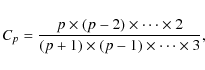
and for odd values of p,
When p=0, we have Cp=1. When p goes to infinity, Cp goes to zero. Setting p=2m for even values of p, and p=2m-1 for odd values (
The cosine power law
![]() was introduced in Stenflo (1987)
to investigate the Zeeman effect with random magnetic fields that may
become predominantly vertical. It was used in Sampoorna et al. (2008b)
to construct a composite PDF that mimics a distribution becoming more
and more vertical as the field strength increases. When p=0, the
distribution is isotropic. When p increases the field becomes more
and more vertical. In the limit
was introduced in Stenflo (1987)
to investigate the Zeeman effect with random magnetic fields that may
become predominantly vertical. It was used in Sampoorna et al. (2008b)
to construct a composite PDF that mimics a distribution becoming more
and more vertical as the field strength increases. When p=0, the
distribution is isotropic. When p increases the field becomes more
and more vertical. In the limit
![]() ,
the Hanle effect
disappears because the scattering atoms are illuminated by an
unpolarized field, cylindrically symmetrical about the magnetic field
direction. This effect is illustrated in Fig. 3. We see
that the ratio
,
the Hanle effect
disappears because the scattering atoms are illuminated by an
unpolarized field, cylindrically symmetrical about the magnetic field
direction. This effect is illustrated in Fig. 3. We see
that the ratio
![]() increases with
p. It reaches the Rayleigh limit when p=1000. The mean Stokes
parameters,
increases with
p. It reaches the Rayleigh limit when p=1000. The mean Stokes
parameters,
![]() and
and
![]() ,
have been calculated in the
micro-turbulent limit, for a magnetic field with constant strength,
corresponding to a Hanle factor
,
have been calculated in the
micro-turbulent limit, for a magnetic field with constant strength,
corresponding to a Hanle factor
![]() .
.
6 Dependence of the polarization on the correlation length
To examine the dependence of the polarization on the
correlation length ![]() (in Doppler width units), we examined
the surface value of the ratio
(in Doppler width units), we examined
the surface value of the ratio
![]() at the limb
(
at the limb
(![]() ),
),
![]() and
and
![]() being the mean values of
Stokes Q and I, for several values of
being the mean values of
Stokes Q and I, for several values of ![]() and T.
and T.
We first chose the simplest PDF, namely an isotropic
angular distribution with a Dirac distribution
![]() .
The
parameter
.
The
parameter
![]() was set to unity. We found that the
dependence of
was set to unity. We found that the
dependence of
![]() on the value of
on the value of ![]() is quite weak for optically thin (
is quite weak for optically thin (![]() )
lines, and also optically thick
(
)
lines, and also optically thick
(![]() )
ones. For lines with a moderate optical depth (T=10),
some dependence could be observed, the maximum variation of the ratio
)
ones. For lines with a moderate optical depth (T=10),
some dependence could be observed, the maximum variation of the ratio
![]() being about 0.1%.
being about 0.1%.
Keeping the assumption of a single value field strength, we
calculated the ratio
![]() for the sine and cosine
power law distributions (see Table 1). For the sine power
law, we chose p=50. For this value of p, the distribution is
strongly peaked in the horizontal direction. For the cosine power
law, we retained p=5. The distribution is also strongly peaked, but in
the vertical direction (see Fig. 11 in Sampoorna et al. 2008b) and the
diminution of the Hanle effect is significant (see
Fig. 3). For these two distributions, the dependence on
the correlation length is also negligible for optically thin and optically
thick lines. Some dependence appears for lines with an intermediate
optical depth. Figure 4, corresponding to the sine
power law and T=10, shows that the difference
for the sine and cosine
power law distributions (see Table 1). For the sine power
law, we chose p=50. For this value of p, the distribution is
strongly peaked in the horizontal direction. For the cosine power
law, we retained p=5. The distribution is also strongly peaked, but in
the vertical direction (see Fig. 11 in Sampoorna et al. 2008b) and the
diminution of the Hanle effect is significant (see
Fig. 3). For these two distributions, the dependence on
the correlation length is also negligible for optically thin and optically
thick lines. Some dependence appears for lines with an intermediate
optical depth. Figure 4, corresponding to the sine
power law and T=10, shows that the difference
![]() all along the
polarization profile. The variation in
all along the
polarization profile. The variation in
![]() is coming almost exclusively from the variation in
is coming almost exclusively from the variation in
![]() ,
since the dependence of Stokes I on the magnetic field is very
small for the Hanle effect. This figure also shows that the
micro-turbulent limit is reached for
,
since the dependence of Stokes I on the magnetic field is very
small for the Hanle effect. This figure also shows that the
micro-turbulent limit is reached for
![]() .
The reason is
that
.
The reason is
that ![]() only enters in exponential terms, as can be seen in
Eq. (19). For the cosine power law and T=10, we found a
very similar behavior to that shown in Fig. 4, but
the polarization is somewhat stronger because of the reduction of the
Hanle effect.
only enters in exponential terms, as can be seen in
Eq. (19). For the cosine power law and T=10, we found a
very similar behavior to that shown in Fig. 4, but
the polarization is somewhat stronger because of the reduction of the
Hanle effect.
![\begin{figure}
\par\includegraphics[height=7cm,width=8cm]{1696fig4.eps}
\end{figure}](/articles/aa/full_html/2009/25/aa11696-09/img195.png) |
Figure 4:
Dependence of
|
| Open with DEXTER | |
To understand the dependence on the correlation length, we
examined the dependence on ![]() and
and
![]() of the
conditional source function component
of the
conditional source function component
![]() .
This function depends strongly on
.
This function depends strongly on ![]() and
and
![]() ,
with the micro and macro-turbulent limits showing quite different
variation with
,
with the micro and macro-turbulent limits showing quite different
variation with
![]() .
The averaging over
.
The averaging over
![]() eliminates most of the variation with
eliminates most of the variation with ![]() .
Some of it may remain, however, in particular when the angular distribution is
peaked in the horizontal or vertical direction.
.
Some of it may remain, however, in particular when the angular distribution is
peaked in the horizontal or vertical direction.
A very low sensitivity to the value of the correlation length is a
strong indication that the polarization is created locally. For a
line with a very small optical thickness, ![]() ,
photons will
suffer about one scattering and the polarization is well represented
by the so-called single scattering approximation. For very thick
lines, although photons suffer a very large number of scattering events, the
polarization is created near the surface by a few of them.
In these two limits, the polarization thus cannot feel the
correlation length of the magnetic field. For T=10, we have an
intermediate situation with a clear sensitivity to the correlation
length.
,
photons will
suffer about one scattering and the polarization is well represented
by the so-called single scattering approximation. For very thick
lines, although photons suffer a very large number of scattering events, the
polarization is created near the surface by a few of them.
In these two limits, the polarization thus cannot feel the
correlation length of the magnetic field. For T=10, we have an
intermediate situation with a clear sensitivity to the correlation
length.
For the Hanle effect, the polarization can be evaluated by a perturbation method leading to a series expansion in terms of a mean number of scattering events (see HF06). In the next section we show how to construct this expansion. We use it to examine how many terms are needed to reproduce the exact solution and thus give a somewhat quantitative content to the above remarks.
7 A series expansion for the calculation of the polarization
The construction of a series expansion for the calculation of the polarization is possible for the following three reasons: (i) the Hanle polarization is weak; (ii) it is controlled by the anisotropy of the radiation field; (iii) at each scattering a significant amount of polarization is being lost. This last point will be clarified below.
Here, for simplicity we present the perturbation method and discuss its convergence properties for the simple case of a deterministic (or micro-turbulent) magnetic field. We then show how to carry it out for magnetic fields with a finite correlation length and propose a perturbation expansion that is an improved version of the method presented in HF06.
7.1 Construction of the expansion
We start from the standard integral equation for the Hanle effect with
a deterministic magnetic field, namely
In the micro-turbulent limit,
In the deterministic case, if the magnetic field is a constant, the
dependence on the azimuthal angle ![]() can be factored out
as shown in Appendix A. Henceforth we work with
the components
can be factored out
as shown in Appendix A. Henceforth we work with
the components
![]() and to
simplify the notation, the dependence on B is omitted.
These new components satisfy the set of equations
and to
simplify the notation, the dependence on B is omitted.
These new components satisfy the set of equations
with
![\begin{displaymath}\mu \frac {\partial I_Q^K(\tau,x,\mu)}{\partial
\tau}=\varphi(x)\left[I_Q^K(\tau,x,\mu) - S^K_Q(\tau)\right].
\end{displaymath}](/articles/aa/full_html/2009/25/aa11696-09/img202.png)
We first consider the equation for S00. Only S20 appears in the righthand side since K=0 implies Q=Q'=0. For the Hanle effect, the polarization is always weak and its effect on Stokes I may be neglected, at least in a first approximation. Neglecting the contribution from S20, we obtain
The notation
We now replace S00 by
![]() in
the equation for S2Q and obtain
in
the equation for S2Q and obtain
where
The kernel
with
Equation (34) shows that
![]() is the driving term for the polarization.
This suggests solving this equation by the standard method of
successive iterations for Fredholm integral equations of the second
type (Iyanaga & Kawada 1970). For radiative transfer problems, this
method is usually referred to as
is the driving term for the polarization.
This suggests solving this equation by the standard method of
successive iterations for Fredholm integral equations of the second
type (Iyanaga & Kawada 1970). For radiative transfer problems, this
method is usually referred to as ![]() -iteration. The zeroth-order
solution in this iteration scheme is given by
-iteration. The zeroth-order
solution in this iteration scheme is given by
![]() .
The recurrence scheme may be written as
.
The recurrence scheme may be written as
![$\displaystyle + \sum_{Q'}N^2_{QQ'}(\bm B)\int_0^T K^{22}_{Q'}(\tau -\tau')
[\tilde{S}^{2}_{Q'}(\tau')]^{(k-1)}~{\rm d}\tau',$](/articles/aa/full_html/2009/25/aa11696-09/img219.png)
with
It is well known that the ![]() -iteration applied to
Eq. (33) has a very poor convergence rate when T is large
and
-iteration applied to
Eq. (33) has a very poor convergence rate when T is large
and ![]() very small, because the kernel K000 is normalized
to unity and the coefficient N000 almost equal to unity. In
Eq. (34) the situation is radically different because
the kernels
very small, because the kernel K000 is normalized
to unity and the coefficient N000 almost equal to unity. In
Eq. (34) the situation is radically different because
the kernels
![]() have integrals over
have integrals over
![]() which are less than unity, actually they are all equal to 7/10(see e.g. HF06),
and the coefficients
N2Q0(B) are also significantly smaller
than unity when B is not zero. For Rayleigh scattering, the
only non-zero coefficient is N200, which is close to
the depolarization parameter
which are less than unity, actually they are all equal to 7/10(see e.g. HF06),
and the coefficients
N2Q0(B) are also significantly smaller
than unity when B is not zero. For Rayleigh scattering, the
only non-zero coefficient is N200, which is close to
the depolarization parameter
![]() (see Appendix A).
(see Appendix A).
To examine the convergence properties of this iteration
scheme, we can consider a simplified version of
Eq. (34). The righthand side of this equation
contains a driving term, a transport term corresponding to Q'=Q, and
terms coupling
![]() with the
with the
![]() ,
,
![]() .
Neglecting these last terms, we see that the solution at step (k)can be written as a series expansion of the form
.
Neglecting these last terms, we see that the solution at step (k)can be written as a series expansion of the form
![$\displaystyle N^2_{Q0}(\bm B)C^2_0(\tau) +
\sum_{m=1}^{m=k}\left[\frac{7}{10}N^2_{QQ}\right]^m$](/articles/aa/full_html/2009/25/aa11696-09/img226.png)
Here the kernels
For optically thin lines (![]() ), one can approximate
), one can approximate
![]() by
by
![\begin{displaymath}[\tilde {S}^2_Q]^{(k)}(\tau)\simeq
N^2_{Q0}(\bm B)C^2_0(\tau...
...{m=1}^k \left[\frac{7}{10}N^2_{QQ}(\bm B)\right]^m T^m\right].
\end{displaymath}](/articles/aa/full_html/2009/25/aa11696-09/img232.png)
The driving term is dominant and suffices to correctly evaluate the polarization. This is the so-called single scattering approximation.
To examine the case of optically thick lines, we can let
![]() .
If we approximate
.
If we approximate
![]() by a delta function, we
obtain
by a delta function, we
obtain
![\begin{displaymath}[\tilde {S}^2_Q]^{(k)}(\tau)\simeq N^2_{Q0}(\bm B)C^2_0(\tau)...
...sum_{m=1}^k \left[\frac{7}{10}N^2_{QQ}(\bm B)\right]^m\right].
\end{displaymath}](/articles/aa/full_html/2009/25/aa11696-09/img235.png)
This expression shows that a single scattering can also provide a reasonable approximation for optically thick lines. We also see that the smaller N2QQ(B), the better the single scattering approximation and the faster the speed of convergence of the series expansion. We also note that the N2QQ(B) are positive, hence the sum inside the square brackets increases with the value of k.
For lines with very large optical thicknesses, the value of Stokes Q at the surface can be easily related to
![]() .
For these
lines, Q is controlled by the component I20. Using
.
For these
lines, Q is controlled by the component I20. Using
![]() for
for ![]() ,
and the
Eddington-Barbier relation, we obtain
,
and the
Eddington-Barbier relation, we obtain
We have performed a few numerical experiments described below to give a quantitative proof to these predictions.
7.2 Numerical results
Table 2: Number of iterations needed to reproduce the exact solution with a relative error about 10-3 at line center, with the parameters of the magnetic field in Cols. 2 and 3 the same as in Figs. 6 and 7.
![\begin{figure}
\par\includegraphics[height=7cm,width=15cm]{1696fig5.eps}
\end{figure}](/articles/aa/full_html/2009/25/aa11696-09/img239.png) |
Figure 5:
Rayleigh scattering. Convergence history of the expansion
method for the calculation of Q/I shown for |
| Open with DEXTER | |
![\begin{figure}
\par\includegraphics[height=7cm,width=15cm]{1696fig6.eps}
\end{figure}](/articles/aa/full_html/2009/25/aa11696-09/img240.png) |
Figure 6:
Same as Fig. 5 but for a deterministic magnetic
field with
|
| Open with DEXTER | |
![\begin{figure}
\par\includegraphics[height=7cm,width=15cm]{1696fig7.eps}\end{figure}](/articles/aa/full_html/2009/25/aa11696-09/img241.png) |
Figure 7:
Same as Figs. 5 and 6 but for a
micro-turbulent magnetic with an isotropic angular distribution
and single value field strength defined by
|
| Open with DEXTER | |
The computation of the polarization by the series expansion method involves the following steps:
- (i)
- solution of Eq. (33) for
 by an ALI
method and calculation of the corresponding scalar radiation field
by an ALI
method and calculation of the corresponding scalar radiation field
 ;
;
- (ii)
- computation of
 with Eq. (36);
- (iii)
- calculation of the source terms
![$[\tilde{S}^2_Q]^{(k)}$](/articles/aa/full_html/2009/25/aa11696-09/img243.png) ,
with the iterative scheme in Eq. (37), starting from
,
with the iterative scheme in Eq. (37), starting from
 ;
;
- (iv)
- at each step (k), solution of Eq. (32) by a short
characteristic method, calculation of the Stokes parameters with
Eq. (5), and of the ratio
at .
Here
.
Here
![$p=\{\left[{Q}/{I}\right]^2 + \left[{U}/{I}\right]^2\}^{1/2}$](/articles/aa/full_html/2009/25/aa11696-09/img245.png) .
.
The iterations are stopped when r(k)<10-3.
We show in Table 2 the number Nk of iterations
defined by the criterion
r(k)<10-3. We stress
that the value of Nk has nothing to do with the number of
iterations of the PALI method, the latter being controlled by the
choice of the approximate
![]() -operator. In
Figs. 5 to 7 we show the results of our
calculations for T=10 and T=104, Fig. 5 being
devoted to the Rayleigh scattering, Fig. 6 to the
deterministic Hanle effect, and Fig. 7 to the
micro-turbulent case. In each panel we plotted the exact values
of Q/I and a few iteration steps. In the micro-turbulent case,
we plotted
-operator. In
Figs. 5 to 7 we show the results of our
calculations for T=10 and T=104, Fig. 5 being
devoted to the Rayleigh scattering, Fig. 6 to the
deterministic Hanle effect, and Fig. 7 to the
micro-turbulent case. In each panel we plotted the exact values
of Q/I and a few iteration steps. In the micro-turbulent case,
we plotted
![]() .
.
We observe that the series expansion properly converges to the exact
solution, that single scattering provides an approximation that is
much better for T=104 than for T=10, and that the accuracy of this
approximation improves from Rayleigh scattering to a deterministic and
micro-turbulent Hanle effect. These last two points are illustrated in
Fig. 8 where we show the difference
calculated at
The decrease in
![]() from Rayleigh scattering to
micro-turbulent Hanle effect, is directly related to the value of
the elements N2QQ. For Rayleigh scattering, the index Q takes
only the value Q=0 and
from Rayleigh scattering to
micro-turbulent Hanle effect, is directly related to the value of
the elements N2QQ. For Rayleigh scattering, the index Q takes
only the value Q=0 and
![]() (assuming WK=1). For the
Hanle effect, the N2QQ and
(assuming WK=1). For the
Hanle effect, the N2QQ and
![]() are significantly
less than unity. Experiments with different angular distributions
clearly show that a decrease in
are significantly
less than unity. Experiments with different angular distributions
clearly show that a decrease in
![]() induces a decrease
in
induces a decrease
in
![]() .
.
Table 2 also shows clearly that the single scattering approximation is better for optically thin and optically thick lines than for lines with intermediate optical thicknesses. It also shows that this approximation is better for a micro-turbulent magnetic field than for a deterministic one or Rayleigh scattering. We examined the values of Nk at different frequency points along the line profile and found that in the wings they are in general a bit higher than at line center.
![\begin{figure}
\par\includegraphics[height=7cm,width=8cm]{1696fig8.eps}
\end{figure}](/articles/aa/full_html/2009/25/aa11696-09/img254.png) |
Figure 8:
Difference between single scattering (ss) and exact (ex) solution as a
function of the optical thickness T for |
| Open with DEXTER | |
Our last comment concerned the fact that the exact value of Stokes Q is
reached from below in the case of thin to moderately thick slabs and
from above in the case of thick slabs (see Figs. 5 to
8). The transition occurs around T=102 as
shown in Fig. 8. This change of behavior is directly
related to the sign of
![]() ,
determined by a
competition between a limb-darkened outgoing radiation and a
limb-brightened incoming one (see e.g. Trujillo Bueno 2001). For
T=104,
,
determined by a
competition between a limb-darkened outgoing radiation and a
limb-brightened incoming one (see e.g. Trujillo Bueno 2001). For
T=104,
![]() is positive as long as
is positive as long as ![]() is less than
unity and then becomes negative (
is less than
unity and then becomes negative (![]() is assumed to be in the range
is assumed to be in the range
![]() ). Since the sum inside the square bracket in
Eq. (40) increases with k, the value of
). Since the sum inside the square bracket in
Eq. (40) increases with k, the value of
![]() near the surface will also increase with the value of
k. We can then deduce from Eq. (41) that Q is
negative and decreases (increases in absolute value) when kincreases.
near the surface will also increase with the value of
k. We can then deduce from Eq. (41) that Q is
negative and decreases (increases in absolute value) when kincreases.
For T<1,
![]() is negative, so we have the opposite
behavior. Apparently this behavior holds until T becomes around
102 (see Figs. 5 to 8) but we
have no simple approximation for Stokes Q or for
is negative, so we have the opposite
behavior. Apparently this behavior holds until T becomes around
102 (see Figs. 5 to 8) but we
have no simple approximation for Stokes Q or for
![]() ,
in this intermediate range of optical
thicknesses.
,
in this intermediate range of optical
thicknesses.
What should be remembered is that the single scattering approximation can lead to very large errors for Rayleigh scattering, but may be sufficient for the micro-turbulent Hanle effect, especially when the line optical thickness is small or large enough.
7.3 Magnetic field with a finite correlation length
Assuming, as above, that S00 is independent of the polarization and
given by the solution of Eq. (33), the equation for
![]() can be written as (see
Eq. (A.1))
can be written as (see
Eq. (A.1))
![$\displaystyle + \int_0^T \left[K^{22}_{Q'}(\tau -\tau')- L^{22}_{Q'}(\tau
-\tau';\nu)\right]$](/articles/aa/full_html/2009/25/aa11696-09/img261.png)
The iteration scheme defined in Eq. (37) can be carried out on this equation. If, at step (k-1), one knows
8 Dependence of the polarization on the magnetic field vector PDF
This study is carried out for the micro-turbulent limit, because one can expect, from our previous results, that the dependence of the polarization on the shape of the magnetic field PDF will be essentially independent of the value of the correlation length.
![\begin{figure}
\par\includegraphics[height=7cm, width=15cm]{1696fig9.eps}
\end{figure}](/articles/aa/full_html/2009/25/aa11696-09/img264.png) |
Figure 9:
Panel a): profile of
|
| Open with DEXTER | |
![\begin{figure}
\par\includegraphics[height=7cm,width=15cm]{1696fi10.eps}
\end{figure}](/articles/aa/full_html/2009/25/aa11696-09/img266.png) |
Figure 10:
Panel a): variation of the ratio
|
| Open with DEXTER | |
![\begin{figure}
\par\includegraphics[height=7cm,width=15cm]{1696fi11.eps}
\end{figure}](/articles/aa/full_html/2009/25/aa11696-09/img267.png) |
Figure 11:
Panel a): variation of the ratio
|
| Open with DEXTER | |
In the micro-turbulent limit, the mean source vector satisfies
Eq. (20). Here we are dealing with magnetic field
distributions that are cylindrically symmetric about the vertical axis
and a primary source term that is unpolarized. Hence, the matrix
![]() is diagonal and the only source vector components that
are not zero are
is diagonal and the only source vector components that
are not zero are
![]() and
and
![]() .
For their
calculation, carried out here with a standard PALI method, we only
need N000 and
.
For their
calculation, carried out here with a standard PALI method, we only
need N000 and
![]() .
The solution of
Eq. (10), with
.
The solution of
Eq. (10), with
![]() as source term,
yields
as source term,
yields
![]() .
The mean value of Stokes Q is then given by
.
The mean value of Stokes Q is then given by
![]() .
.
The element
![]() can be calculated explicitly for all
the angular distributions given in Table 1, when they are
associated to the delta and Gaussian strength distributions. The
expressions are given in Appendix B. In the
other cases,
can be calculated explicitly for all
the angular distributions given in Table 1, when they are
associated to the delta and Gaussian strength distributions. The
expressions are given in Appendix B. In the
other cases,
![]() is calculated by numerical averaging
with Gauss-Legendre quadratures. We have also considered a
log-normal distribution, but it yields essentially the same results as
the Gaussian distribution.
is calculated by numerical averaging
with Gauss-Legendre quadratures. We have also considered a
log-normal distribution, but it yields essentially the same results as
the Gaussian distribution.
The calculations were performed for slabs with different optical
thickness T and we found that the main conclusions are essentially
independent of the value of T. The results shown in this section
correspond to a slab with parameters
![]() .
.
Figure 9 is devoted to the isotropic distribution.
Panel (a) shows that
![]() increases (in absolute value)
as we go from a Dirac distribution (single field strength value), to
a Maxwell distribution, then a Gaussian distribution, and finally an
exponential distribution, i.e. from case (i) to case (iv) (see
Table 1). All these curves lie well above the Rayleigh
scattering limit in which
increases (in absolute value)
as we go from a Dirac distribution (single field strength value), to
a Maxwell distribution, then a Gaussian distribution, and finally an
exponential distribution, i.e. from case (i) to case (iv) (see
Table 1). All these curves lie well above the Rayleigh
scattering limit in which
![]() .
The
variation of
.
The
variation of
![]() is due to the fact that the value
of
is due to the fact that the value
of
![]() increases as we go from case (i) to case (iv),
because the probability of having weak magnetic fields
increases. The maximum value of
increases as we go from case (i) to case (iv),
because the probability of having weak magnetic fields
increases. The maximum value of
![]() is reached for
Rayleigh scattering.
is reached for
Rayleigh scattering.
In Fig. 9b we show the center-to-limb variation of
![]() .
A striking feature is that the
variation with
.
A striking feature is that the
variation with ![]() is almost insensitive to the field strength
distribution. We have even found that the full line curve,
corresponding to a Dirac PDF with B=B0, coincides exactly with the
center-to-limb variation given by an exponential distribution with a
mean value
is almost insensitive to the field strength
distribution. We have even found that the full line curve,
corresponding to a Dirac PDF with B=B0, coincides exactly with the
center-to-limb variation given by an exponential distribution with a
mean value
![]() .
This result fully agrees with the
calculations of Trujillo Bueno et al. (2004), showing that observed
center-to-limb variations can be fitted by an
isotropic field with a strength of 60 G, or by an exponential
distribution with a mean value of 130 G.
.
This result fully agrees with the
calculations of Trujillo Bueno et al. (2004), showing that observed
center-to-limb variations can be fitted by an
isotropic field with a strength of 60 G, or by an exponential
distribution with a mean value of 130 G.
Somewhat more insight into the behavior of
![]() can be
obtained by considering
can be
obtained by considering
![]() .
The dependence on optical
depth is controlled by the propagation kernel
.
The dependence on optical
depth is controlled by the propagation kernel
![]() (see
Sect. 7). As a result, changing the shape of
(see
Sect. 7). As a result, changing the shape of
![]() will have a very small effect on the
will have a very small effect on the ![]() -dependence of
-dependence of
![]() (see Eq. (41)). In contrast, a change in the shape
of
(see Eq. (41)). In contrast, a change in the shape
of
![]() will modify the value of
will modify the value of
![]() ,
hence the degree of polarization.
,
hence the degree of polarization.
In Fig. 10, devoted to the cosine and sine angular
power laws, we see that the ratio
![]() also increases from case (i) to case (iv). The dependence on the shape
of
also increases from case (i) to case (iv). The dependence on the shape
of
![]() is quite strong for the sine power law with p=50(even a bit more than with the isotropic distribution), but very
small for the cosine power law with p=5. This stems from the
reduction of the Hanle effect when the field becomes strongly peaked
in the vertical direction.
is quite strong for the sine power law with p=50(even a bit more than with the isotropic distribution), but very
small for the cosine power law with p=5. This stems from the
reduction of the Hanle effect when the field becomes strongly peaked
in the vertical direction.
In Fig. 11, we show the ratio
![]() for magnetic fields with different angular
distributions, the field strength being kept equal to a single value
B0. In Fig. 11a, we see that the choice of the
angular distribution has a strong effect on the amplitude of this
ratio, but not on its center-to-limb variation, for the reason given
above. Figure 11b shows the variation in this ratio
with the Hanle efficiency parameter
for magnetic fields with different angular
distributions, the field strength being kept equal to a single value
B0. In Fig. 11a, we see that the choice of the
angular distribution has a strong effect on the amplitude of this
ratio, but not on its center-to-limb variation, for the reason given
above. Figure 11b shows the variation in this ratio
with the Hanle efficiency parameter
![]() for
for ![]() ,
x=0, and
,
x=0, and ![]() .
We observe the standard Hanle saturation for
large field strengths. An isotropic distribution, and a sine power law
with a fairly horizontally peaked distribution, yield similar
polarizations, as already been pointed out in Stenflo (1982).
There are, however, observable differences around
.
We observe the standard Hanle saturation for
large field strengths. An isotropic distribution, and a sine power law
with a fairly horizontally peaked distribution, yield similar
polarizations, as already been pointed out in Stenflo (1982).
There are, however, observable differences around
![]() .
The
polarization is higher for the cosine power law because the
distribution is strongly peaked in the vertical direction.
.
The
polarization is higher for the cosine power law because the
distribution is strongly peaked in the vertical direction.
These numerical experiments with different magnetic field PDFs indicate a clear sensitivity of the polarization to the magnetic field strength and angular distributions. Hence, any information on mean magnetic field strengths, extracted from Hanle depolarization measurements, may depend critically on the choice of the magnetic field PDF that has been made a priori for the analysis of the observations.
9 Concluding remarks
In this paper, we have studied the Hanle effect due to a random magnetic field with a finite correlation length, in order to assess limitations to the usual micro-turbulent approximation. The modeling of the magnetic field by a Markovian random process, piecewise constant, characterized by a correlation length and a magnetic field vector probability density function (PDF), enabled us to construct a radiative transfer equation for a mean radiation field, which still depends on the random values of the magnetic field (Sect. 3). A simple averaging of the solution of this equation over the PDF yields the mean Stokes parameters. The transfer equation is solved numerically by a PALI method, generalized to the problem at hand (Sect. 4).
We find that optically thin lines (lines with optical thickness
![]() ), and very optically thick ones (
), and very optically thick ones (![]() )
can be treated
with the micro-turbulent approximation. For these lines, the
polarization is created locally by a small number of scattering
events. For optically thick lines they are located near the
surface. To evaluate this number of events, the polarization has been
calculated by a method of successive iterations leading to a series
expansion in the mean number of scattering events
(Sect. 7). For optically thin and thick lines,
this number is around 5; for lines with intermediate optical
thicknesses (
)
can be treated
with the micro-turbulent approximation. For these lines, the
polarization is created locally by a small number of scattering
events. For optically thick lines they are located near the
surface. To evaluate this number of events, the polarization has been
calculated by a method of successive iterations leading to a series
expansion in the mean number of scattering events
(Sect. 7). For optically thin and thick lines,
this number is around 5; for lines with intermediate optical
thicknesses (
![]() -100), it is significantly more (10-15)
and these lines show some sensitivity to the magnetic field
correlation length (see Fig. 4).
-100), it is significantly more (10-15)
and these lines show some sensitivity to the magnetic field
correlation length (see Fig. 4).
We also find that for a random magnetic field, the single scattering approximation can be safely used to evaluate the Hanle depolarization. For a deterministic magnetic field, it may also provide a reasonable approximation. In contrast, for the Rayleigh scattering, it may lead to large errors, except for optically thin lines (see Fig. 8).
Numerical experiments carried out in the micro-turbulent limit, with different types of magnetic field PDF, indicate that the polarization is quite sensitive to the shape of the PDF (Sect. 8). However, our results suggest that it may not be easy to retrieve a quiet Sun magnetic field PDF from the Hanle effect depolarization measurements, since the same degree of linear polarization can be created by PDFs that have rather different shapes. The center-to-limb variation of the linear polarization also depends very little on the PDF shape. Several laws for the solar magnetic field PDF have been proposed in recent years. They have been deduced from Zeeman effect measurements and may contain some uncertainty in the weak field domain involved in the Hanle effect. Numerical simulations such as those carried out in Schüssler & Vögler (2008) may clarify the situation.
In this paper, we have complete frequency redistribution at each scattering. This assumption is certainly not valid to analyze the Hanle depolarization of strong resonance lines showing significant partial redistribution effects. An example is the Ba ii D2 line considered in Faurobert et al. (2009) to evaluate the turbulent magnetic field in the low chromosphere. However, our conclusions concerning the applicability of the micro-turbulent approximation remain most probably valid, since the polarization is still created in a small region close to the surface. The transfer equations given here and their method of solution can be easily generalized to handle partial frequency redistribution and to verify this prediction, but this generalization will be accompanied by a significant increase in computing time.
Acknowledgements
The authors have greatly benefited from discussions with V. Bommier and J. O. Stenflo. L.S.A. is grateful to the Laboratoire Cassiopée (Université de Nice, OCA, CNRS) for financial support and hospitality during a stay in Nice where part of this work was completed.
Appendix A: Integral equations for the components of the source vector
In Eqs. (17) to (19) of the text, we give
the integral equation for the source vector
![]() .
The corresponding system of integral equations for
its KQ components
.
The corresponding system of integral equations for
its KQ components
![]() may be written as
may be written as
with
The
with
with
We recall that
![\begin{displaymath}X_{KQ''}(B)= \frac{W_K(J_{\rm l},J_{\rm u})}{1 + \epsilon +\d...
...(K)}_{\rm u}}\left
[\frac{1}{1 + Q''\Gamma'_{B}}\right ]\cdot
\end{displaymath}](/articles/aa/full_html/2009/25/aa11696-09/img292.png)
Here
Equation (A.4) shows that the ![]() dependence of the
dependence of the
![]() appears as a phase factor. This
suggests introducing a new function
appears as a phase factor. This
suggests introducing a new function
![]() defined by the relation
defined by the relation
The integral equation for this new function is
This equation becomes simpler if the magnetic field PDF is cylindrically symmetrical with respect to the z-axis, i.e. of the form
We can integrate over
We note here that the term involving the mean value of SK'Q'is zero when
Once the
![]() have been calculated, they have to
be multiplied by
have been calculated, they have to
be multiplied by
![]() (see Eq. (A.7))
and then averaged over the magnetic field PDF. Since
P(B) has
been assumed to have a cylindrical symmetry, the averaging process
will give zero, except for the components with Q=0, so the mean
source vector
(see Eq. (A.7))
and then averaged over the magnetic field PDF. Since
P(B) has
been assumed to have a cylindrical symmetry, the averaging process
will give zero, except for the components with Q=0, so the mean
source vector
![]() and mean Stokes vector
and mean Stokes vector
![]() only have two non-zero
components corresponding to K=0,2 and Q=0. The magnetic field PDF
does not break the cylindrically symmetry of the atmosphere. We stress
that there is no way to avoid the calculations of the
only have two non-zero
components corresponding to K=0,2 and Q=0. The magnetic field PDF
does not break the cylindrically symmetry of the atmosphere. We stress
that there is no way to avoid the calculations of the
![]() components with
components with ![]() .
The reason is that
the integral equation for the conditional mean source vector holds for
both the micro and macro-turbulent limits.
.
The reason is that
the integral equation for the conditional mean source vector holds for
both the micro and macro-turbulent limits.
Appendix B: Exact expressions of the mean coefficient

The coefficient
N200 is defined in the
Appendix A. Exact expressions for the mean values
![]() can obtained with the PDFs given in
Table 1, when the magnetic field strength has a Dirac or Gaussian
distribution. Because of the cylindrical symmetry of the PDFs,
can obtained with the PDFs given in
Table 1, when the magnetic field strength has a Dirac or Gaussian
distribution. Because of the cylindrical symmetry of the PDFs,
![]() .
The expressions given below
correspond to WK=1 and
.
The expressions given below
correspond to WK=1 and
![]() .
.
When the field strength has a Dirac distribution, the coefficents
![]() have the form
have the form
![\begin{displaymath}\left\langle N^2_{\rm {00}} \right\rangle_{\rm D} =
{\frac{1...
...4\Gamma '^{2}_{B}}{1+4\Gamma
'^{2}_{B}}} \right) \right]\cdot
\end{displaymath}](/articles/aa/full_html/2009/25/aa11696-09/img323.png)
The coefficients C1 and C2 only depend on the angular distribution. The coefficient
When the field strength has a Gaussian distribution,
![\begin{displaymath}\left\langle N^2_{00} \right\rangle_{\rm G}={\frac{1}{1+\epsilon}}
\left[1-C_{1}K_{1} - C_{2}K_{2}\right].
\end{displaymath}](/articles/aa/full_html/2009/25/aa11696-09/img325.png)
The coefficients Km , m=1,2, may be written as
![\begin{displaymath}K_m=1-\left[{\frac{\sqrt{\pi}}{m\gamma_\sigma}}\exp\left({\fr...
...ht)
{\rm erfc}\left({\frac{1}{m\gamma_\sigma}}\right)\right],
\end{displaymath}](/articles/aa/full_html/2009/25/aa11696-09/img326.png)
with

One can check that the coefficients K1 and K2 go to zero when the magnetic field goes to zero.
We give in Table B.1 the coefficients C1 and C2 for the isotropic, cosine, and sine power laws defined in Table 1, Col. 2, of the text. Some of these results can be found in Stenflo (1994, Eq. (10.54),1982).
For p=0, C1 and C2 go to 2/5 and we recover the isotropic angular distribution. For the cosine power law, when p goes to infinity, C1 and C2 go to zero and we recover the Rayleigh scattering. For the sine power law, when p goes to infinity, C1 goes to zero and C2 to 0.75.
Table B.1:
Coefficients C1 and C2 for the calculation of
![]() .
.
References
- Auer, L. H., & Paletou, F. 1994, A&A, 285, 675 [NASA ADS]
- Auvergne, M., Frisch, H., Frisch, U., Froeschlé, Ch., & Pouquet, A. 1973, A&A, 29, 93 [NASA ADS] (In the text)
- Bommier, V. 1997, A&A, 328, 726 [NASA ADS]
- Bommier, V., Derouich, M., Landi Degl'Innocenti, E., Molodij, G., & Sahal-Bréchot, S. 2005, A&A, 432, 295 [NASA ADS] [CrossRef] [EDP Sciences]
- Brissaud, A., & Frisch, U. 1971, JQSRT, 11, 1767 [NASA ADS] [CrossRef] (In the text)
- Brissaud, A., & Frisch, U. 1974, J. Math. Phys., 15, 524 [NASA ADS] [CrossRef] (In the text)
- Dominguez Cerdena, I., Sánchez Almeida, J., & Kneer, F. 2006, ApJ, 646, 1421 [NASA ADS] [CrossRef]
- Carroll, T. A., & Staude, J. 2005, Astron. Nachr., 326, 296 [NASA ADS] [CrossRef] (In the text)
- Faurobert-Scholl, M. 1991, A&A, 246, 469 [NASA ADS]
- Faurobert-Scholl, M. 1993, A&A, 268, 765 [NASA ADS]
- Faurobert-Scholl, M. 1996, Sol. Phys. 164, 79
- Faurobert, M., Arnaud, J., Vigneau, J., & Frisch, H. 2001, A&A, 378, 627 [NASA ADS] [CrossRef] [EDP Sciences]
- Faurobert, M., Derouich, M., Bommier, V., & Arnaud, J. 2009, A&A, 493, 201 [NASA ADS] [CrossRef] [EDP Sciences]
- Fluri D. M., Nagendra K. N., & Frisch H. 2003, A&A, 400, 303 [NASA ADS] [CrossRef] [EDP Sciences]
- Frisch, H. 2006, A&A, 446, 403 [NASA ADS] [CrossRef] [EDP Sciences] (HF06) (In the text)
- Frisch, H. 2007, A&A, 476, 665 [NASA ADS] [CrossRef] [EDP Sciences] (HF07)
- Frisch, H., & Frisch, U. 1975, in Colloque International du CNRS, ed. R. Cayrel, & M. Steinberg (Editions du CNRS), 250, 113 (In the text)
- Frisch, H., & Frisch, U. 1976, MNRAS, 175, 157 [NASA ADS] (In the text)
- Iyanaga, S., & Kawada, Y. 1970, Encyclopedic Dictionary of Mathematics (Cambridge, Massachusetts: The MIT Press) (In the text)
- Kunasz, P. B., & Auer, L. H. 1988, JQSRT, 39, 67 [NASA ADS] [CrossRef]
- Landi Degl'Innocenti, E. 1984, Sol. Phys., 91, 1 [NASA ADS] [CrossRef] (In the text)
- Landi Degl'Innocenti, E., & Bommier, V. 1994, A&A, 284, 865 [NASA ADS] (In the text)
- Landi Degl'Innocenti, E., & Landolfi, M. 2004, Polarization in Spectral Lines (Kluwer Academic Publishers) (LL04) (In the text)
- Landi Degl'Innocenti, E., Bommier, V., & Sahal-Bréchot, S. 1990, A&A, 235, 459 [NASA ADS] (In the text)
- Léger, L., Chevallier, L., & Paletou, F. 2007, A&A, 470, 1 [NASA ADS] [CrossRef] [EDP Sciences]
- Lites, B., Kubo, M., Socas-Navarro, H., et al. 2008, ApJ, 672, 1237 [NASA ADS] [CrossRef] (In the text)
- Manso Sainz, R., & Trujillo Bueno, J. 1999, ASSL Ser., 243, Solar Polarization, ed. K. N. Nagendra, & J. O. Stenflo, 143
- Manso Sainz, R., & Trujillo Bueno, J. 2003, ASP Conf. Ser. 307, ed. J. Trujillo Bueno, & J. Sánchez Almeida, 251
- Nagendra, K. N., Frisch, H., & Faurobert-Scholl, M. 1998, A&A, 332, 610 [NASA ADS]
- Nagendra, K. N., Paletou, F., Frisch, H., & Faurobert-Scholl, M. 1999, Solar Polarization II, ed. K. N. Nagendra, & J. O. Stenflo (Boston: Kluwer Academic Publishers), 127
- Nagendra, K. N., & Sampoorna, M. 2009, in Solar Polarization 5, ed. S. V. Berdyugina, K. N. Nagendra, & R. Ramelli, ASP Conf. Ser., 405, 261 (In the text)
- Papoulis, A. 1965, Probability, Random Variables, and Stochastic Processes (New York: Mac Graw Hill) (In the text)
- Sampoorna, M., Nagendra, K. N., & Frisch, H. 2008a, JQSRT, 109, 2349 [NASA ADS]
- Sampoorna, M., Nagendra, K. N., Frisch, H., & Stenflo, J. O. 2008b, A&A, 485, 275 [NASA ADS] [CrossRef] [EDP Sciences]
- Sánchez Almeida, J. 2007, ApJ, 657, 1150 [NASA ADS] [CrossRef]
- Schüssler, M., & Vögler, A. 2008, A&A, 481, L5 [NASA ADS] [CrossRef] [EDP Sciences] (In the text)
- Stenflo, J. O. 1982, Sol. Phys., 80, 209 [NASA ADS] [CrossRef] (In the text)
- Stenflo, J. O. 1987, Sol. Phys., 114, 1 [NASA ADS]
- Stenflo, J. O. 1994, Solar Magnetic Fields (Dordrecht: Kluwer) (In the text)
- Stenflo, J. O. 2009, in Astrophys. Space Science Proceedings, Magnetic coupling between the Interior and Atmospheres of the Sun, ed. S. S. Hasan, & R. J. Rutten, in press (In the text)
- Stoer, J., & Bulirsch, R. 1983, Introduction to Numerical Analysis (Springer-Verlag) (In the text)
- Trujillo Bueno, J. 2001, in Advanced Solar Polarimetry Theory, Observation, and Instrumentation, ed. M. Sigwarth, ASP Conf. Ser., 236, 161 (In the text)
- Trujillo Bueno, J., & Fabiani Bendicho, P. 1995, ApJ, 455, 646 [NASA ADS] [CrossRef]
- Trujillo Bueno, J., Shchukina, N., & Asensio Ramos, A. 2004, Nature, 430, 326 [NASA ADS] [CrossRef]
All Tables
Table 1: A list of different PDFs used in this paper.
Table 2: Number of iterations needed to reproduce the exact solution with a relative error about 10-3 at line center, with the parameters of the magnetic field in Cols. 2 and 3 the same as in Figs. 6 and 7.
Table B.1:
Coefficients C1 and C2 for the calculation of
![]() .
.
All Figures
| |
Figure 1:
Atmospheric reference frame with the definition of ( |
| Open with DEXTER | |
| In the text | |
| |
Figure 2:
Probability density functions
|
| Open with DEXTER | |
| In the text | |
| |
Figure 3:
Effect of the cosine power-law index p on
|
| Open with DEXTER | |
| In the text | |
| |
Figure 4:
Dependence of
|
| Open with DEXTER | |
| In the text | |
| |
Figure 5:
Rayleigh scattering. Convergence history of the expansion
method for the calculation of Q/I shown for |
| Open with DEXTER | |
| In the text | |
| |
Figure 6:
Same as Fig. 5 but for a deterministic magnetic
field with
|
| Open with DEXTER | |
| In the text | |
| |
Figure 7:
Same as Figs. 5 and 6 but for a
micro-turbulent magnetic with an isotropic angular distribution
and single value field strength defined by
|
| Open with DEXTER | |
| In the text | |
| |
Figure 8:
Difference between single scattering (ss) and exact (ex) solution as a
function of the optical thickness T for |
| Open with DEXTER | |
| In the text | |
| |
Figure 9:
Panel a): profile of
|
| Open with DEXTER | |
| In the text | |
| |
Figure 10:
Panel a): variation of the ratio
|
| Open with DEXTER | |
| In the text | |
| |
Figure 11:
Panel a): variation of the ratio
|
| Open with DEXTER | |
| In the text | |
Copyright ESO 2009
Current usage metrics show cumulative count of Article Views (full-text article views including HTML views, PDF and ePub downloads, according to the available data) and Abstracts Views on Vision4Press platform.
Data correspond to usage on the plateform after 2015. The current usage metrics is available 48-96 hours after online publication and is updated daily on week days.
Initial download of the metrics may take a while.