| Issue |
A&A
Volume 501, Number 1, July I 2009
|
|
|---|---|---|
| Page(s) | 171 - 187 | |
| Section | Extragalactic astronomy | |
| DOI | https://doi.org/10.1051/0004-6361/200809883 | |
| Published online | 05 May 2009 | |
Simulations of galactic disks including a dark baryonic component
Y. Revaz1,2 - D. Pfenniger3 - F. Combes2 - F. Bournaud4
1 - Laboratoire d'Astrophysique, École Polytechnique Fédérale de Lausanne (EPFL), 1290 Sauverny, Switzerland
2 -
LERMA, Observatoire de Paris, 61 Av. de l'Observatoire, 75014 Paris, France
3 -
Geneva Observatory, University of Geneva, 1290 Sauverny, Switzerland
4 -
Laboratoire AIM, CEA-Saclay DSM/DAPNIA/SAp-CNRS-Université Paris Diderot, 91191 Gif-Sur-Yvette, France
Received 1 April 2008 / Accepted 4 April 2009
Abstract
The near proportionality between HI and dark matter in outer galactic
disks prompted us to run N-body simulations of galactic disks in which
the observed gas content is supplemented by a dark gas component
representing between zero and five times the visible gas content.
While adding baryons in the disk of galaxies may solve some issues, it
poses the problem of disk stability.
We show that the global stability is ensured if the ISM is multiphased, composed of two
partially coupled phases, a visible warm gas phase and a weakly
collisionless cold dark phase corresponding to a fraction of the
unseen baryons. The phases are subject to stellar and UV background
heating and gas cooling, and their transformation into each other is
studied as a function of the coupling strength.
This new model, which still possesses a dark matter halo, fits
the rotation curves as well as the classical CDM halos,
but is the only one to explain the existence of an open and contrasting spiral structure,
as observed in the outer HI disks
Key words: galaxies: evolution - galaxies: ISM - galaxies: structure - galaxies: general - galaxies: kinematics and dynamics
1 Introduction
The ![]() CDM scenario encounters much success in reproducing
the large scale structures of the Universe traced by the
Lyman-
CDM scenario encounters much success in reproducing
the large scale structures of the Universe traced by the
Lyman-![]() forest and gravitational lensing (Springel et al. 2006).
However, at galactic scale, where the baryonic physics plays a major
role, the
forest and gravitational lensing (Springel et al. 2006).
However, at galactic scale, where the baryonic physics plays a major
role, the ![]() CDM scenario has several well known
problems. The dark matter cusp in galaxies
(Swaters et al. 2003; de Blok & Bosma 2002; de Blok et al. 2008; Gentile et al. 2005; Blais-Ouellette et al. 2001; de Blok 2005; Spano et al. 2008; Spekkens et al. 2005; Gentile et al. 2004), and in
particular in dwarf irregulars, the high number of small systems
orbiting halos (Strigari et al. 2007; Moore et al. 1999; Klypin et al. 1999), the low angular
momentum problem at the origin of too small disks
(Navarro & Steinmetz 1997; Kaufmann et al. 2007; Navarro & Benz 1991), as well as the difficulty of
forming bulgeless disks (Mayer et al. 2008) suggest that some physics is
missing.
CDM scenario has several well known
problems. The dark matter cusp in galaxies
(Swaters et al. 2003; de Blok & Bosma 2002; de Blok et al. 2008; Gentile et al. 2005; Blais-Ouellette et al. 2001; de Blok 2005; Spano et al. 2008; Spekkens et al. 2005; Gentile et al. 2004), and in
particular in dwarf irregulars, the high number of small systems
orbiting halos (Strigari et al. 2007; Moore et al. 1999; Klypin et al. 1999), the low angular
momentum problem at the origin of too small disks
(Navarro & Steinmetz 1997; Kaufmann et al. 2007; Navarro & Benz 1991), as well as the difficulty of
forming bulgeless disks (Mayer et al. 2008) suggest that some physics is
missing.
A strong prediction of the ![]() CDM scenario is that the so called
``missing baryons'' reside in a warm-hot gas phase in the over-dense
cosmic filaments (Cen & Ostriker 2006,1999). However, there are now several
theoretical and observational arguments that support the fact that
galactic disks may be more massive than usually thought, containing a
substantial fraction of these ``missing baryons''.
CDM scenario is that the so called
``missing baryons'' reside in a warm-hot gas phase in the over-dense
cosmic filaments (Cen & Ostriker 2006,1999). However, there are now several
theoretical and observational arguments that support the fact that
galactic disks may be more massive than usually thought, containing a
substantial fraction of these ``missing baryons''.
It has been pointed out by Bosma (1981,1978) that in samples of galaxies, the ratio between the dark matter and HI surface density is roughly constant well after the optical disk (see also Broeils 1992; Hoekstra et al. 2001; Carignan et al. 1990). This correlation may be a direct consequence of the conservation of the specific angular momentum of the gas during the galaxy formation process (Seiden et al. 1984). However, as shown by van den Bosch (2001) the angular momentum conservation leads to the formation of too concentrated stellar disks, a real problem for the low surface brightness galaxies. On the other hand, the HI-dark matter correlation may suggest that a large fraction of the dark matter lies in the disk of galaxies, following the HI distribution. This physical link between HI and dark matter has been confirmed by the baryonic Tully-Fischer relation of spiral galaxies (Pfenniger & Revaz 2005) and more recently for extremely low mass galaxies (Begum et al. 2008).
Dark matter in the disk of galaxies is now also suggested by dynamical arguments based on the asymmetries of galaxies, either in the plane of the disks or transverse to it. For example, the large spiral structure present in the very extended HI disk of NGC 2915 is supported by a quasi self-gravitating disk (Masset & Bureau 2003; Bureau et al. 1999). Revaz & Pfenniger (2004) have shown that heavy disks are subject to vertical instabilities (also called bending instabilities) and may generate all types of observed warps: the common S-shaped but also the U-shaped and asymmetric ones (Sánchez-Saavedra et al. 2003; Reshetnikov & Combes 1999). Other arguments for the origin of warps have been proposed (Jiang & Binney 1999; Shen & Sellwood 2006; Weinberg & Blitz 2006), however none of them are able to explain the three types of warps.
Several works have tried to study the flattening of the Milky Way halo
using potential tracers like dwarf galaxies (Johnston et al. 2005). From
theses studies, the halo potential appears to be nearly spherical,
with an ellipticity of 0.9. However, dwarf galaxies trace the halo
at distances larger than
![]() where it is difficult to
distinguish ``classical'' CDM disks with a slightly flattened halo
from a heavy disk model, containing half of the halo mass in an
extended flat disk (Revaz & Pfenniger 2007).
where it is difficult to
distinguish ``classical'' CDM disks with a slightly flattened halo
from a heavy disk model, containing half of the halo mass in an
extended flat disk (Revaz & Pfenniger 2007).
A more accurate method is to trace the potential near the plane of the
disk, using for example the vertical gas distribution.
Kalberla (2004); Kalberla et al. (2007); Kalberla (2003) have modeled the HI
distribution out to a galactic radius of
![]() .
Their
self-consistent model is compatible with a self-gravitating dark
matter disk having a mass of 2-
.
Their
self-consistent model is compatible with a self-gravitating dark
matter disk having a mass of 2-
![]()
![]() .
.
The presence of dark baryons in the disk of galaxies is reinforced by the numerous signs of recent star formation in the far outer disk of galaxies, correlated with HI gas in NGC 6946 (Ferguson et al. 1998), NGC 628 (Lelièvre & Roy 2000), M 101 Smith et al. (2000), M 31 Cuillandre et al. (2001), NGC 6822 (de Blok & Walter 2003), M 83 (Thilker et al. 2005). Correlations between young stars and HI far from the center reveal that molecular gas, at the origin of a weak but existing star formation rate, must be present in abundance there, despite the lack of CO detection.
Other arguments supporting the idea that dark matter could reside in
the galactic disk in the form of cold molecular hydrogen (![]() )
have
been widely discussed by Pfenniger et al. (1994).
)
have
been widely discussed by Pfenniger et al. (1994).
Unfortunately, a direct detection of cold ![]() in the outer disk of
galaxies appears to be a very hard task (Combes & Pfenniger 1997). As the
in the outer disk of
galaxies appears to be a very hard task (Combes & Pfenniger 1997). As the
![]() molecule is symmetrical, any electric dipole moment is
canceled. The molecule may be detected in emission only by its
quadrupole radiation, the lowest corresponding to a temperature of
molecule is symmetrical, any electric dipole moment is
canceled. The molecule may be detected in emission only by its
quadrupole radiation, the lowest corresponding to a temperature of
![]() above the fundamental state, much above the
5-7 K expected from Pfenniger & Combes (1994). A weak radiation of
the
above the fundamental state, much above the
5-7 K expected from Pfenniger & Combes (1994). A weak radiation of
the ![]() ultra-fine lines is expected at kilometer wavelengths.
However, since it is 10 orders of magnitude smaller than the HI line
for the same density, its detection will not be possible in the
near future. The absorption lines may be the best way to detect
ultra-fine lines is expected at kilometer wavelengths.
However, since it is 10 orders of magnitude smaller than the HI line
for the same density, its detection will not be possible in the
near future. The absorption lines may be the best way to detect
![]() .
But this method requires large statistics, as the filling
factor of the gas is expected to be very low (<
.
But this method requires large statistics, as the filling
factor of the gas is expected to be very low (<![]() ).
).
The best tracers of cold ![]() may be the pure
rotational lines of
may be the pure
rotational lines of ![]() (at 28, 17, 12 and 9 microns), which
could be emitted by a few percent of the molecular gas, excited by
intermittent turbulence (see for example Boulanger et al. 2008).
(at 28, 17, 12 and 9 microns), which
could be emitted by a few percent of the molecular gas, excited by
intermittent turbulence (see for example Boulanger et al. 2008).
Indirect detection by tracers may be prone to error. For example, CO
traces the ![]() but only for enriched gas and fails at large
distances from galaxy centers. Moreover, it is impossible to detect
CO emission from a cloud at a temperature close to the background
temperature. The cold dust component detected by COBE/IRAS
(Reach et al. 1995) is known to trace the cold
but only for enriched gas and fails at large
distances from galaxy centers. Moreover, it is impossible to detect
CO emission from a cloud at a temperature close to the background
temperature. The cold dust component detected by COBE/IRAS
(Reach et al. 1995) is known to trace the cold ![]() .
But as for the
CO, it is limited to small galactic radii where the cold gas is still
mixed with some dust. Spitzer mid-infrared observations have recently
revealed that large quantities of molecular hydrogen are not
associated with star formation (Appleton et al. 2006; Ogle et al. 2007). An
unexpectedly large amount of
.
But as for the
CO, it is limited to small galactic radii where the cold gas is still
mixed with some dust. Spitzer mid-infrared observations have recently
revealed that large quantities of molecular hydrogen are not
associated with star formation (Appleton et al. 2006; Ogle et al. 2007). An
unexpectedly large amount of
![]() of H2 is revealed
only by its strong H2 emission lines in the galaxy Zwicky 3146
(Egami et al. 2006). Grenier et al. (2005) showed that much gas in the solar
neighborhood is revealed only by
of H2 is revealed
only by its strong H2 emission lines in the galaxy Zwicky 3146
(Egami et al. 2006). Grenier et al. (2005) showed that much gas in the solar
neighborhood is revealed only by ![]() -rays. Other indirect
detections could be possible using micro-lensing events
(Fux 2005; Draine 1998). However, this method has not been exploited up
to now.
-rays. Other indirect
detections could be possible using micro-lensing events
(Fux 2005; Draine 1998). However, this method has not been exploited up
to now.
As direct and indirect observational detection of cold gas is difficult, it is necessary to test the effect a cold gas component would have on the global evolution of galactic disks. In this paper, we present new N-body simulations of galactic disks, where the observed gas content has been multiplied by a factor between 3 and 5. In addition to this extra dark baryonic component, a non-baryonic, spheroidal pressure-supported dark halo containing most of the large-scale dark mass is conserved.
An important issue that our model aims to answer is the stability question of heavy disks (Elmegreen 1997). Our model assumes that the additional baryons lie in a very cold and clumpy phase (Pfenniger & Combes 1994), partially dynamically decoupled from the visible dissipative phase. We show that this phase can thus be less dissipative than the visible ISM and has larger velocity dispersions, so that the global disk stability is preserved. A new numerical implementation of the cycling acting between these two phases is proposed.
The secular evolution shows that the models with additional baryons are globally stable and share on average the same observational properties as the ``classical'' CDM disks. However, they give a natural explanation for the presence of contrasting spiral structures in the outskirts of HI disks which is difficult to explain when taking into account the self-gravity of the HI alone. In a forthcoming paper, we will show that this model also reproduces the puzzling dark matter content present in debris from galaxies (Bournaud et al. 2007).
Our model is different from previous multiphase models (Merlin & Chiosi 2007; Harfst et al. 2006; Semelin & Combes 2002) in the sense that it does not compute a cycling between a cold-warm dissipative and hot medium, but between a very cold weakly collisional phase and the visible dissipative phase.
The paper is organized as follows. Details of the multiphase model is given in Sect. 2. In Sect. 3 we briefly discuss the parameters used, and Sect. 4 is devoted to the galaxy model description. Section 5 compares the evolution of galaxy models with and without additional baryons and a short discussion. A summary is given in Sect. 6.
2 The multiphase model
2.1 The straightforward approach
The straightforward approach when modelling the galactic ISM is to
assume that gas behaves like an ideal, inviscid gas. The evolution of
the specific energy u of the gas may be obtained by inserting the
continuity equation into the first law of thermodynamics:
The first right hand side term corresponds to the adiabatic behavior of the gas, while the second is responsible for the entropy variation. This latter reflects the non-adiabatic processes included through the heating and cooling function
However, the ISM is known to be strongly non homogeneous down to very
small scales, reaching densities higher than
![]()
![]() where the cooling time is very short, leading to
equilibrium temperatures below
where the cooling time is very short, leading to
equilibrium temperatures below
![]() .
Such over-densities are
unfortunately far from being resolved by galactic scale simulations
and numerical simulations miss the associated low temperatures.
While being physically correct, Eq. (1) will then strongly bias
the equilibrium temperature of the gas, because the estimated average
density
.
Such over-densities are
unfortunately far from being resolved by galactic scale simulations
and numerical simulations miss the associated low temperatures.
While being physically correct, Eq. (1) will then strongly bias
the equilibrium temperature of the gas, because the estimated average
density ![]() poorly reflects the actual physics.
poorly reflects the actual physics.
2.2 Statistical approach
Instead of following the thermal specific energy of particles using the biased Eq. (1), we propose a new statistical approach avoiding the problem of the density and temperature evaluation. The multiphase ISM is assumed to be a two level system (see Fig. 1) with probabilities of transition depending only on the local excitation energy flux, that we call for short ``UV flux'', which is assumed to be the dominant heating process.
The top level is populated by the well known observed dissipative gas detected by its CO, H2 or HI emission. This phase will be called the visible gas. The bottom level is populated by undetected very clumpy and cold gas as proposed by Pfenniger & Combes (1994), having temperature below the CO detection limit, at temperature equilibrium with the cosmic background radiation. This gas results from the strong cooling that occurs in overdense regions. As this gas is missed by all tracers, we will call it the dark gas.
According to the astrophysical literature, we have used here the word ``gas''. However, it is well known that the cold interstellar medium shows fractal properties which have been observed up to the instrumental capabilities, down to a few hundred AU (Heithausen 2004). Such heterogeneous fluids clearly do not have the viscosity or other mean properties of smooth flows. In other fields, it would be called granular flows, for example. We are aware of the degree of simplification of our model compared to the complexity of the ISM. A more complex model should include the dark component, the CO-undetected metal-poor warmer H2 gas that may exist in the outskirts of galactic disks (Papadopoulos et al. 2002), and possible effects related to phase transition and separation in the He-H2 mixture at very cold temperature (Safa & Pfenniger 2008).
![\begin{figure}
\par\begin{picture}
(0,0)%
\includegraphics{schema.pstex} %
\end{...
...ult}{\color[rgb]{0,0,0}$\chi_{\rm{ext}}$ }%
}}}} }
\end{picture}%\end{figure}](/articles/aa/full_html/2009/25/aa09883-08/img37.png) |
Figure 1:
Schematic representation of the ISM two levels system. The visible gas is labeled VG, the dark gas DG and the stars ST. The probability of transition between the visible and the dark gas depends on the UV flux generated by young stars (
|
| Open with DEXTER | |
The transition times between visible and dark gas is only dependent on
the local UV flux ![]() ,
which is the main heating process in the
ISM. For the transition times, we have chosen the following simple
relations:
,
which is the main heating process in the
ISM. For the transition times, we have chosen the following simple
relations:
 |
(2) |
where

where in these latter equations, we have defined
2.3 Visible and dark gas dynamics
The visible phase is assumed to be dissipative, because it is more diffuse
and collisional than the cold phase. Instead of using the classical
SPH approach, which makes the gas strongly collisional, we have
preferred to use the sticky particle scheme
(Brahic 1977; Schwarz 1981; Combes & Gerin 1985) which better simulates the clumpy
ISM. In the following simulations, we have used
![]() and
and
![]() in order to strictly conserve angular
momentum
in order to strictly conserve angular
momentum![]() . The frequency of
collisions between particles is set to be proportional to the local
visible gas density.
. The frequency of
collisions between particles is set to be proportional to the local
visible gas density.
Also, as the very cold and clumpy dark gas does not radiate, it is expected to be weakly collisional. Its relaxation time being much longer than the dynamical time, we neglect here the effect of collisions.
2.4 Star formation
Stars that are assumed to be the main source of UV flux in the inner part of the galaxy may be formed out of the visible gas only. We have used a classical star formation recipe (Katz et al. 1996) that reproduces well the Schmidt law.
2.5 UV flux
The normalized UV energy flux ![]() is decomposed into two parts. A
stellar radiation flux
is decomposed into two parts. A
stellar radiation flux
![]() and an extragalactic background
energy flux
and an extragalactic background
energy flux
![]() .
.
2.5.1 Stellar UV flux
The stellar normalized radiation flux is computed by summing the
contribution of each star, assuming an appropriate (L/M) ratio.
where mi is the particle of mass i and ri its distance to the point where the flux is estimated.
2.5.2 Extragalactic UV flux
The extragalactic UV background normalized radiation flux is assumed
to be constant.
 |
(7) |
where the extragalactic UV background density is set to
Table 1: Multiphase model parameters.
3 Parameters
Our multiphase model is based on 4 parameters. The external energy
density flux
![]() ,
the UV light to mass ratio (L/M), the
coefficient parameter
,
the UV light to mass ratio (L/M), the
coefficient parameter ![]() and the time scale of transition
and the time scale of transition ![]() .
In this paper, we have fixed the 4 parameters to constant values given
in Table 1.
The parameter
.
In this paper, we have fixed the 4 parameters to constant values given
in Table 1.
The parameter ![]() is set to 1 for simplicity. The
parameter (L/M) is chosen such that the normalized stellar UV flux
is set to 1 for simplicity. The
parameter (L/M) is chosen such that the normalized stellar UV flux
![]() is unity near
is unity near
![]() when the stellar
distribution at the origin of the UV flux corresponds to a realistic
exponential disk, as will be presented in
Sect. 4. According to Eq. (5), these
values correspond to the radius where the dark component surface
density is equivalent to the visible surface density.
when the stellar
distribution at the origin of the UV flux corresponds to a realistic
exponential disk, as will be presented in
Sect. 4. According to Eq. (5), these
values correspond to the radius where the dark component surface
density is equivalent to the visible surface density.
![]() is chosen such that, in the absence of a stellar UV field (at a distance
is chosen such that, in the absence of a stellar UV field (at a distance
![]() from the galaxy center), the ratio
from the galaxy center), the ratio
![]() where
where
![]() has been
set to 1/10. From Eq. (3) and setting
has been
set to 1/10. From Eq. (3) and setting
![]() we get:
we get:
 |
(8) |
The time scale of the transition
![\begin{figure}
\par\includegraphics[width=9cm,clip]{9883Fig01.eps}
\end{figure}](/articles/aa/full_html/2009/25/aa09883-08/img76.png) |
Figure 2:
Normalized UV flux |
| Open with DEXTER | |
4 Galaxy models
We have used our multiphase model to simulate the evolution of Milky
Way-like spiral galaxies. In order to understand the effect of the
multiphase model, we have compared two models, including additional
dark baryons, with a reference ``classical'' model. In addition, we
have build a fourth simulation including the perturbation of
![]() CDM substructures. In the following sections, we first
present our reference model (also called N=1 model), where no
additional dark baryons have been added. In the next section (Sect. 4.1.2) we present how it is possible to add
dark baryons in the reference model, in a way consistent with the
rules proposed in Chapter 2 and by conserving the
same observational properties of the reference model. The model
including
CDM substructures. In the following sections, we first
present our reference model (also called N=1 model), where no
additional dark baryons have been added. In the next section (Sect. 4.1.2) we present how it is possible to add
dark baryons in the reference model, in a way consistent with the
rules proposed in Chapter 2 and by conserving the
same observational properties of the reference model. The model
including ![]() CDM substructures will be presented in
Sect. 4.1.3. Section 4.2
will discuss how initial velocities have been set in order to make the
disk stable.
CDM substructures will be presented in
Sect. 4.1.3. Section 4.2
will discuss how initial velocities have been set in order to make the
disk stable.
4.1 Mass distribution
4.1.1 The reference model
Our reference model is designed to fit typical properties of giant Sbc galaxies with a flat extended rotation curve. It is initially composed of a bulge, an exponential stellar disk, a gas disk and a dark matter halo.
- 1.
- The bulge density profile is a simple Plummer model:
with a characteristic radius .
.
- 2.
- The exponential stellar disk takes the usual form:
where the radial and vertical scale length are respectively HR=4 and .
.
- 3.
- The dark matter is distributed in a Plummer model:
with a characteristic radius ,
ensuring a
flat rotation curve up to
,
ensuring a
flat rotation curve up to
 .
The model is truncated at
.
The model is truncated at
 (
(
 ). In order to avoid any perturbation
of the halo on the disk due to imperfect equilibrium, we have set it
as a rigid potential. We have checked that a live halo will not
influence our results.
). In order to avoid any perturbation
of the halo on the disk due to imperfect equilibrium, we have set it
as a rigid potential. We have checked that a live halo will not
influence our results.
- 4.
- The choice of the visible gas distribution follows the observations of
Hoekstra et al. (2001), where the dark matter contribution to the rotation
curve is a multiple of the contribution of the gas. This is achieved
by distributing the gas in a Miyamoto-Nagai model (Miyamoto & Nagai 1975):
The proportionality between the Plummer halo (being in fact a subclass of a Miyamoto-Nagai model) and the disk is ensured if the disk scale length is similar to the one of the halo: (see
Appendix A). The vertical scale height hz is fixed
to
(see
Appendix A). The vertical scale height hz is fixed
to
 .
We also have included a flaring of the visible
gas disk by multiplying the z coordinates of the particles by:
.
We also have included a flaring of the visible
gas disk by multiplying the z coordinates of the particles by:
where the transition radius is set to
.
is set to
.

Table 2: Parameters for the reference giant Sbc model.
![\begin{figure}
\par\includegraphics[width=8.9cm,clip]{9883Fig02.eps}
\end{figure}](/articles/aa/full_html/2009/25/aa09883-08/img93.png) |
Figure 3: Rotation curve of the reference model with the contribution of each component, the bulge, the exponential disk, the visible gas and the dark matter halo. |
| Open with DEXTER | |
4.1.2 Adding dark baryons in the disk
Here, we present a method that allows us to build new galaxy models containing additional dark baryons, but presenting similar observational properties as the reference model. The new models are build by following three rules:
- 1.
- the total rotation curve remains nearly unchanged with respect to the reference model;
- 2.
- the surface density of the visible gas remains nearly unchanged with respect to the reference model;
- 3.
- no dynamically significant dark matter is added in the central regions.
The third rule is derived from the luminosity Milky-Way model
(Bissantz & Gerhard 2002) combined with MACHO micro-lensing observations (see
Gerhard 2006, and references therein for more details). We thus
assume 1) no dark gas exists at the center of galaxies, and 2) the
density of the total gas (tg) is equal to that of the visible gas
(vg):
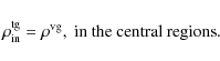
This equation also ensures the second rule at the center.
In the outer part, the total gas mass distribution is constrained by
the first rule. We can easily transfer mass from the halo to the disk
without changing the rotation curve, using the equivalence in term of
density of Eq. (A.5) (via the Poisson equation). In
that case, the density of the halo plus the total gas (htg) (including
visible and dark gas) may be written as:
where the first left side term corresponds to the total gas density:
and the second left side term corresponds to the halo density:
In this equation, the mass of each component is given as an index.
 |
(18) |
where N gives the ratio between the total gas and the gas of the reference model. Its value is restricted to the range
We can derive the total gas density all along the disk by combining
Eqs. (14) and (16):
where we have introduced a new function
We now introduce the multiphase model of
Sect. 2 that places constraints on the ratio
between visible and dark gas. Applying Eq. (4) to the total
gas density
![]() we can derive the density of the visible
gas:
we can derive the density of the visible
gas:
and where
In this equation, we force values of
Following this scheme, we have constructed two different models, with respectively N=3 and N=5. Applying the multiphase model with parameters listed in Table 1, we can now determine the mass properties of the different components (visible gas, dark gas, total baryons and dark halo) in these models, including the reference model (N=1), given in Table 3.
A larger value of N increases the dark mass and inversely decreases
the dark halo mass (the total mass remaining constant). The baryon
fraction (
![]() /
/
![]() )
is then an increasing function
of N and grows from the universal baryonic fraction up to
)
is then an increasing function
of N and grows from the universal baryonic fraction up to ![]() for
model N=5. The total visible mass is not strictly identical between
the three models. Its variation is mainly due to the the outer part
where its surface density decreases with respect to the reference
model. However, the visible gas lying below
for
model N=5. The total visible mass is not strictly identical between
the three models. Its variation is mainly due to the the outer part
where its surface density decreases with respect to the reference
model. However, the visible gas lying below
![]() is similar
for the 3 models (
is similar
for the 3 models (
![]() ).
).
The gas and total baryon surface density is displayed in
Figs. 4 and 5. The outer regions
(
![]() )
of models N=3 and N=5 are characterised by the
presence of the dark gas which dominates the surface density of the
baryons. In the far outer parts, the baryons are multiplied by N,
with respect to the reference model. On the contrary, due to the drop
in the dark gas surface density, the visible gas surface density of
the inner regions is left unchanged with respect to the reference
model (second rule). The presence of dark gas is only marginal inside
)
of models N=3 and N=5 are characterised by the
presence of the dark gas which dominates the surface density of the
baryons. In the far outer parts, the baryons are multiplied by N,
with respect to the reference model. On the contrary, due to the drop
in the dark gas surface density, the visible gas surface density of
the inner regions is left unchanged with respect to the reference
model (second rule). The presence of dark gas is only marginal inside
![]() .
.
Table 3: Parameters for the reference giant Sbc model.
![\begin{figure}
\par\includegraphics[width=8.9cm,clip]{9883Fig03.eps}
\end{figure}](/articles/aa/full_html/2009/25/aa09883-08/img120.png) |
Figure 4: Comparison of the surface density of baryons between model N=1 and model N=3. The total baryons (including stars) are traced in black. The red line represents the visible gas while the blue line (only present for the N=3 model) falling towards the center corresponds to the dark gas. |
| Open with DEXTER | |
Figures 6 and 7 compare the contribution of all
components to the rotation curve. In the models with additional
baryons, the decreasing contribution of the dark halo mass in the
outer part is compensated by the dark gas, ensuring a flat rotation
curve up to
![]() .
The bump in this component,
appearing below
.
The bump in this component,
appearing below
![]() ,
is due to the fact that, as no dark gas
resides in the central regions, the square velocity of this component
alone is negative. As in Figs. 6 and 7 we have
plotted the absolute value of the velocity, the imaginary part appears
as positive.
Except around the transition radius of
,
is due to the fact that, as no dark gas
resides in the central regions, the square velocity of this component
alone is negative. As in Figs. 6 and 7 we have
plotted the absolute value of the velocity, the imaginary part appears
as positive.
Except around the transition radius of
![]() ,
the total rotation
curve of models N=3 and N=5 remains nearly unchanged with respect
to the reference model (first rule).
,
the total rotation
curve of models N=3 and N=5 remains nearly unchanged with respect
to the reference model (first rule).
![\begin{figure}
\par\includegraphics[width=8.9cm,clip]{9883Fig04.eps}
\end{figure}](/articles/aa/full_html/2009/25/aa09883-08/img123.png) |
Figure 5: Same figure as Fig. 4 but for model N=5. |
| Open with DEXTER | |
![\begin{figure}
\par\includegraphics[width=8.9cm,clip]{9883Fig05.eps} \end{figure}](/articles/aa/full_html/2009/25/aa09883-08/img124.png) |
Figure 6: Comparison of the rotation curves of model N=1 and model N=3 and the contribution of each component. |
| Open with DEXTER | |
![\begin{figure}
\par\includegraphics[width=8.9cm,clip]{9883Fig06.eps}
\end{figure}](/articles/aa/full_html/2009/25/aa09883-08/img125.png) |
Figure 7: Same figure as Fig. 6 but for model N=5. |
| Open with DEXTER | |
4.1.3  CDM substructures
In addition to the three previous models, we have built a fourth model
called the N=1+s model based on the N=1 models but taking
into account a sample of dark matter satellites predicted by the
![]() CDM cosmology, orbiting around the disk and interacting with
it.
CDM cosmology, orbiting around the disk and interacting with
it.
The purpose of this model is to study the effect of ![]() CDM
satellites on the spiral structure of the disk, and to compare it with
the effect of the additional baryons taken into account in models
N=3 and N=5.
CDM
satellites on the spiral structure of the disk, and to compare it with
the effect of the additional baryons taken into account in models
N=3 and N=5.
The ![]() CDM satellites have been added following the technique
described by Gauthier et al. (2006) based on the distribution function of
Gao et al. (2004), in agreement with recent
CDM satellites have been added following the technique
described by Gauthier et al. (2006) based on the distribution function of
Gao et al. (2004), in agreement with recent ![]() CDM simulations.
100 satellites extending up to
CDM simulations.
100 satellites extending up to
![]() ,
with masses between
,
with masses between
![]() and 0.02 mass of the galaxy of the reference
model (
and 0.02 mass of the galaxy of the reference
model (
![]() ), have been added,
representing
), have been added,
representing ![]() of the total galactic mass. Contrary to
Gauthier et al. (2006), in our simulations, the substructures are Plummer
masses with a softening fixed to
of the total galactic mass. Contrary to
Gauthier et al. (2006), in our simulations, the substructures are Plummer
masses with a softening fixed to
![]() .
Figure 8 shows the surface density of model N=1+sincluding the
.
Figure 8 shows the surface density of model N=1+sincluding the ![]() CDM satellites. The darkness of the satellites
scales as a function of the mass.
CDM satellites. The darkness of the satellites
scales as a function of the mass.
| |
Figure 8:
Model N=1+s: 100 |
| Open with DEXTER | |
4.2 Velocity distribution
The velocity distributions are computed following the method proposed
by Hernquist (1993). For the spherical distribution, the bulge,
the velocity dispersion is assumed to be isotropic and is derived from
the second moment of the Jeans equation (Binney & Tremaine 1987) which is
then:
For the axisymmetric components (stellar disk and gas disk), we first compute the vertical velocity dispersion
For the stellar disk and for the bulge, the radial velocity dispersion
where
where the rotation frequency
where we have assumed that the term
4.2.1 Velocity distribution for the visible and dark gas
The radial velocity dispersions of the visible gas is set to be
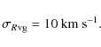
constant at 10 km s-1 as observed:
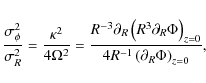
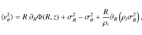
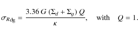
On the contrary, in order to ensure stability, the radial velocity dispersions of the dark gas is set by imposing the Savronov-Toomre parameter to be 1:
The velocity dispersions and the mean azimuthal velocity are then used to distribute the model particles in the velocity space.
5 Model evolution
The multiphase model has been implemented on the parallel Tree code
Gadget2 (Springel 2005). The models N=1, N=1+s, N=3 and
N=5 contain respectively 319 315, 319 415, 535 769 and 731 129particles. The mass of the gas particles is constant between the
three models. The softening length is set to
![]() .
All
simulations have been run between 0 and
.
All
simulations have been run between 0 and
![]() .
For
simplicity, the feedback from supernovae has been turned off.
.
For
simplicity, the feedback from supernovae has been turned off.
5.1 Global properties
Despite their different dark matter content, after
![]() ,
the three models (N=1, N=3 and N=5) still share similar global
properties.
,
the three models (N=1, N=3 and N=5) still share similar global
properties.
In Fig. 9 we compare the total velocity curve
of the three models, after
![]() of evolution. In the
central part, they all show a bump corresponding to the presence of a
bar. In the outer part, all curves converge to the same values. The
main differences occur around the transition radius (
of evolution. In the
central part, they all show a bump corresponding to the presence of a
bar. In the outer part, all curves converge to the same values. The
main differences occur around the transition radius (![]()
![]() ), where models with additional baryons have slightly
lower values. However, these differences are simply a relic of the
differences existing in the initial conditions (see Figs. 6
and 7). The similarity of the rotation curves means that
the three models share the same radial potential dependency, having
similar horizontal epicyclic frequencies (
), where models with additional baryons have slightly
lower values. However, these differences are simply a relic of the
differences existing in the initial conditions (see Figs. 6
and 7). The similarity of the rotation curves means that
the three models share the same radial potential dependency, having
similar horizontal epicyclic frequencies (![]() and
and ![]() ). The
pattern speed, the shape and the extension of the bar is also
identical (see Fig. 10).
). The
pattern speed, the shape and the extension of the bar is also
identical (see Fig. 10).
![\begin{figure}
\par\includegraphics[width=8.9cm,clip]{9883Fig08.eps}
\end{figure}](/articles/aa/full_html/2009/25/aa09883-08/img152.png) |
Figure 9:
Comparison of the rotation curve of the 3 models at
|
| Open with DEXTER | |
| |
Figure 10:
Surface density map of the stellar disk of the 3 models (N=1, N=3 and N=5, from left to right) at
|
| Open with DEXTER | |
The surface density of the three models is compared in
Fig. 11. For radius smaller than
![]() ,
the curves corresponding to the visible gas surface
density are superimposed. Differentiating these three curves is only
possible in the far outer part, as was the case for the
initial conditions (see Figs. 4 and 5).
It is thus important to notice that the rotation curve and the
azimuthal averaged surface density are not sufficient to easily
distinguish between these three models, even after
,
the curves corresponding to the visible gas surface
density are superimposed. Differentiating these three curves is only
possible in the far outer part, as was the case for the
initial conditions (see Figs. 4 and 5).
It is thus important to notice that the rotation curve and the
azimuthal averaged surface density are not sufficient to easily
distinguish between these three models, even after
![]() of
evolution.
of
evolution.
![\begin{figure}
\par\includegraphics[width=8.9cm,clip]{9883Fig10.eps}
\end{figure}](/articles/aa/full_html/2009/25/aa09883-08/img156.png) |
Figure 11:
Comparison of the surface density of different components at
|
| Open with DEXTER | |
![\begin{figure}
\par\includegraphics[width=8.9cm,clip]{9883Fig11.eps}
\end{figure}](/articles/aa/full_html/2009/25/aa09883-08/img158.png) |
Figure 12:
Disk scale height as a function of the radius, for the four models at t=0.9 and
|
| Open with DEXTER | |
![\begin{figure}
\par\includegraphics[width=8.8cm,clip]{9883Fig12.eps}
\end{figure}](/articles/aa/full_html/2009/25/aa09883-08/img160.png) |
Figure 13:
Evolution of model N=1 between 0 and
|
| Open with DEXTER | |
![\begin{figure}
\par\includegraphics[width=8.8cm,clip]{9883Fig13.eps}
\end{figure}](/articles/aa/full_html/2009/25/aa09883-08/img162.png) |
Figure 14:
Evolution of model N=1 including 100 |
| Open with DEXTER | |
![\begin{figure}
\par\includegraphics[width=15.95cm,clip]{9883Fig14.eps}
\end{figure}](/articles/aa/full_html/2009/25/aa09883-08/img163.png) |
Figure 15:
Evolution of model N=3 between 0 and
|
| Open with DEXTER | |
![\begin{figure}
\par\includegraphics[width=15.9cm,clip]{9883Fig15.eps}
\end{figure}](/articles/aa/full_html/2009/25/aa09883-08/img164.png) |
Figure 16:
Evolution of model N=5 between 0 and
|
| Open with DEXTER | |
In Fig. 12 we compare the scale height of the disk of
the four models at t=0.9 and at
![]() .
The continuous
lines correspond to the visible gas while the dotted ones to the dark
gas. At
.
The continuous
lines correspond to the visible gas while the dotted ones to the dark
gas. At
![]() ,
no difference exists between the four
models. After
,
no difference exists between the four
models. After
![]() of evolution the visible gas in the
N=1+s, N=3 and N=5 models has been slightly heated and presents higher
scale heights. In the case of model N=1+s, the increase of the scale
height is attributed to the perturbation of the
of evolution the visible gas in the
N=1+s, N=3 and N=5 models has been slightly heated and presents higher
scale heights. In the case of model N=1+s, the increase of the scale
height is attributed to the perturbation of the ![]() CDM
satellites (Dubinski et al. 2008; Font et al. 2001), while for models N=3 and N=5it is due to the coupling with the collisionless dark gas that has a
higher scale height (dotted lines). From an observational point of
view, models N=1+s, N=3 and N=5 will be very similar.
CDM
satellites (Dubinski et al. 2008; Font et al. 2001), while for models N=3 and N=5it is due to the coupling with the collisionless dark gas that has a
higher scale height (dotted lines). From an observational point of
view, models N=1+s, N=3 and N=5 will be very similar.
5.2 Disk stability and spiral structures
The main differences between the models with additional dark baryons
and the ``classical model'' appear when comparing the spiral structure
of the visible gas.
The surface density evolution of the three models
plus the one with the ![]() CDM satellites is displayed in
Figs. 13-16. In the two latter plots, in addition to the
visible gas surface density, the dark gas surface density is also
displayed. These plots emphasize two important points. First, despite
the presence of larger amount of baryons in the outer parts, the disks
of models N=3 and N=5 are globally stable over the 4.5 simulated
Gyrs. Secondly, spiral structures have very different patterns and
may be used to distinguish between models with and without additional
baryons.
CDM satellites is displayed in
Figs. 13-16. In the two latter plots, in addition to the
visible gas surface density, the dark gas surface density is also
displayed. These plots emphasize two important points. First, despite
the presence of larger amount of baryons in the outer parts, the disks
of models N=3 and N=5 are globally stable over the 4.5 simulated
Gyrs. Secondly, spiral structures have very different patterns and
may be used to distinguish between models with and without additional
baryons.
At all times during the evolution, the surface density of the dark gas decreases at the center, preserving a
hole. This hole simply means that no additional dark matter is
expected at the center, even after
![]() of evolution.
of evolution.
5.2.1 Disk stability
The stability of models N=3 and N=5 is ensured by the presence of the two partially dynamically decoupled phases. The dark phase has higher velocity dispersions than the visible gas. The radial velocity dispersions of model N=3 are displayed in Fig. 17. Because the dark gas is quasi non-collisional, its radial velocity dispersion is much larger than the one of the visible gas of the reference model (values dropping to 10 km s-1 in the outer part.). These higher values ensure the stability of the total baryonic disk. However, our multiphase model fails to reproduce the low velocity dispersions expected in the visible gas. While being clearly decoupled from the dark component, the gas velocity dispersion of model N=3 is higher than the one of the reference model, especially in the outer part. This is the result of the weak coupling due to the cycling between the dark and the visible gas. The model could be improved in the future, by simply increasing the stickiness of particles in the outer part.
As discussed in Appendix B, if one assumes that the dark gas is as dissipative as the visible gas, the resulting velocity dispersions of the total gas is no longer large enough to ensure the disk stability. In that case, the disk breaks and forms small clumps (Fig. B.1).
Since our disk model is made of three dynamically decoupled
components (the stellar disk, the visible disk and the dark disk)
having distinct velocity dispersions, a precise study of its stability
would require to use a multi-component stability criterion. The
stability of multi-component galactic disks has been discussed by
Jog & Solomon (1984a,b) and the equivalent of the Savronov-Toomre
parameter may be computed (Jog 1996). While this criterion is
theoretically valid for an n-components system the computational
procedure described by Jog (1996) is only valid for a
two-components system (see also Wang & Silk 1994; and
Elmegreen 1995). We have instead used a Savronov-Toomre
(
![]() )
assuming a single component. Formally, this
)
assuming a single component. Formally, this
![]() is defined by:
is defined by:
where
5.3 Spiral structure and swing amplification
While being larger than 1, the two models with additional baryons
are characterized by a nearly constant
![]() from 10 to
from 10 to
![]() ,
with values between 2 and 3 for model N=3 and
around 2 for model N=5. With these rather low values, the disks
are only quasi-stable. Contrasting and open spiral structures are
continuously generated up to the end of the dark gas disk at
,
with values between 2 and 3 for model N=3 and
around 2 for model N=5. With these rather low values, the disks
are only quasi-stable. Contrasting and open spiral structures are
continuously generated up to the end of the dark gas disk at
![]() .
These spirals are thus naturally present in the
visible gas up to its end, where its surface density drops, in
agreement with most HI observed disks. See for example the
impressive case of NGC 6946 (Boomsma et al. 2008).
.
These spirals are thus naturally present in the
visible gas up to its end, where its surface density drops, in
agreement with most HI observed disks. See for example the
impressive case of NGC 6946 (Boomsma et al. 2008).
![\begin{figure}
\par\includegraphics[width=9cm,clip]{9883Fig16.eps}
\end{figure}](/articles/aa/full_html/2009/25/aa09883-08/img172.png) |
Figure 17:
Radial velocity dispersion at
|
| Open with DEXTER | |
![\begin{figure}
\par\includegraphics[width=9cm,clip]{9883Fig17.eps}
\end{figure}](/articles/aa/full_html/2009/25/aa09883-08/img174.png) |
Figure 18:
Stability of models N=1, N=3 and N=5 at different
times (0, 0.9, 1.8, 2.3, 3.2 and
|
| Open with DEXTER | |
![\begin{figure}
\par\includegraphics[width=8.5cm,clip]{9883Fig18.eps}
\end{figure}](/articles/aa/full_html/2009/25/aa09883-08/img175.png) |
Figure 19:
Evolution of the spiral structure in a ( |
| Open with DEXTER | |
On the contrary, model N=1 has a higher
![]() ,
increasing
well above 3 for
,
increasing
well above 3 for
![]() .
Consequently, the outer disk is
more stable, preventing the formation of spirals, as observed in
Fig. 13. This difference is the key point that
allow us to distinguish between models with and without additional
baryons.
.
Consequently, the outer disk is
more stable, preventing the formation of spirals, as observed in
Fig. 13. This difference is the key point that
allow us to distinguish between models with and without additional
baryons.
In order to improve our understanding of the spiral structure, we have
computed polar maps ((![]() -plot) of the visible gas surface
density (from R=0 to
-plot) of the visible gas surface
density (from R=0 to
![]() )
at different times
(Fig. 19). These maps can be, for example, compared to
the HI observation in M 83 (Fig. 12 of Crosthwaite et al. 2002).
We then performed a Fourier decomposition of those maps, for each
radius. The spiral structure can be represented by each dominant
azimuthal modes for a given radius, i.e. the mode with the largest
amplitude, excluding the m=0 mode. Figure 20 displays the
amplitude of the dominant azimuthal modes found for each plot of
Fig. 19. For a direct comparison between the models, in
all plots, the signal amplitude is coded with the same colors.
In polar plots, a regular spiral structure of mode m appears as
2 m inclined parallel lines
)
at different times
(Fig. 19). These maps can be, for example, compared to
the HI observation in M 83 (Fig. 12 of Crosthwaite et al. 2002).
We then performed a Fourier decomposition of those maps, for each
radius. The spiral structure can be represented by each dominant
azimuthal modes for a given radius, i.e. the mode with the largest
amplitude, excluding the m=0 mode. Figure 20 displays the
amplitude of the dominant azimuthal modes found for each plot of
Fig. 19. For a direct comparison between the models, in
all plots, the signal amplitude is coded with the same colors.
In polar plots, a regular spiral structure of mode m appears as
2 m inclined parallel lines![]() , where the inclination (that may vary with
radius) gives the pitch angle i of the arm (
, where the inclination (that may vary with
radius) gives the pitch angle i of the arm (
![]() (p), where p is the slope of the lines). Such regular
features are present for the N=3 and N=5 models, indicating the
presence of rather open spiral arms (large i) that may be followed
up to
(p), where p is the slope of the lines). Such regular
features are present for the N=3 and N=5 models, indicating the
presence of rather open spiral arms (large i) that may be followed
up to
![]() at nearly all times. The number of arms is not
constant and oscillates between 3 and 8 (model N=3) and 3 and
6 (model N=5), usually increasing with increasing radius
(Bottema 2003). Such large features are not observed for the N=1model. The spiral arms disappear around
at nearly all times. The number of arms is not
constant and oscillates between 3 and 8 (model N=3) and 3 and
6 (model N=5), usually increasing with increasing radius
(Bottema 2003). Such large features are not observed for the N=1model. The spiral arms disappear around
![]() .
.
Spiral arms in a disk may be the result of ``swing
amplification'' (Goldreich & Lynden-Bell 1965; Toomre 1981; Julian & Toomre 1966), a mechanism that
locally enhances the self-gravity and leads to the amplification of a
small perturbation in a differentially rotating structure. The
amplification results from the resonance between the epicyclic motions
of stars (or gas) and the rate of change of the pitch angle of a
density wave, during its conversion from leading to trailing
(Binney & Tremaine 1987).
The swing amplification mechanism may be quantified by the parameter
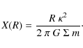
X, the ratio of the perturbation wavelength and a critical
wavelength:

Since the wavelength
Similarly to the
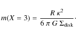
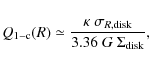
The meaning of the critical mode is the following: modes higher than m(X=3) may be amplified by the swing amplification mechanism. On the contrary, the ones above m(X=3) are stable and thus no spiral pattern with m<m(X=3) is observed.
![\begin{figure}
\par\includegraphics[width=8.9cm,clip]{9883Fig19.eps}
\end{figure}](/articles/aa/full_html/2009/25/aa09883-08/img188.png) |
Figure 20:
Evolution of the spiral structure in a ( |
| Open with DEXTER | |
The right panels of Fig. 18 displays the critical modes at
different times. For the N=1 model, m(X=3) increases very
quickly, being above 6 for
![]() .
At larger radii, only
large m modes, corresponding to noise, may be amplified by the
self-gravity of the disk. No spiral pattern is expected, in agreement
with Figs. 20 and 13.
.
At larger radii, only
large m modes, corresponding to noise, may be amplified by the
self-gravity of the disk. No spiral pattern is expected, in agreement
with Figs. 20 and 13.
When increasing
![]() by including additional baryons,
self-gravity in increased and lower modes may be amplified at larger
radius. For example, m=6 modes may still be amplified up to
by including additional baryons,
self-gravity in increased and lower modes may be amplified at larger
radius. For example, m=6 modes may still be amplified up to
![]() in model N=3 and up to
in model N=3 and up to
![]() in model
N=5. This explains the patterns present in
Fig. 20 and the spiral structure of
Figs. 15 and 16.
in model
N=5. This explains the patterns present in
Fig. 20 and the spiral structure of
Figs. 15 and 16.
The dotted lines of Fig. 18 (both in the left and right panels)
correspond to the
![]() and m(X=3) values as would be
deduced by an observer ignoring the presence of the dark gas and
taking into account only the visible gas and stars in Eqs. (30)
and (33). Clearly,
and m(X=3) values as would be
deduced by an observer ignoring the presence of the dark gas and
taking into account only the visible gas and stars in Eqs. (30)
and (33). Clearly,
![]() is well above 4 for a radius
larger than
is well above 4 for a radius
larger than
![]() ,
indicating that the disk should be stable.
The m(X=3) parameter implies that modes with low
perturbation should be prohibited by the swing amplification theory,
in contradiction to the observed spiral structure. This point may
explain why spiral structures are present in galaxies where the
,
indicating that the disk should be stable.
The m(X=3) parameter implies that modes with low
perturbation should be prohibited by the swing amplification theory,
in contradiction to the observed spiral structure. This point may
explain why spiral structures are present in galaxies where the
![]() (or X) parameter deduced from the visible component
is well above 5 (resp. 3), as is the case, for example, for the
galaxy NGC 2915 (Bureau et al. 1999).
(or X) parameter deduced from the visible component
is well above 5 (resp. 3), as is the case, for example, for the
galaxy NGC 2915 (Bureau et al. 1999).
5.3.1 The effect of the CDM satellites
We can now ask if the perturbations generated by the ![]() CDM
satellites are able to reproduce the large scale spiral patterns of
galaxies, comparable with the ones obtained when including additional
baryons.
CDM
satellites are able to reproduce the large scale spiral patterns of
galaxies, comparable with the ones obtained when including additional
baryons.
The effect of the satellites may be seen by comparing the surface
density of the visible gas disk of model N=1(Fig. 13) and model N=1+s(Fig. 14). Perturbations in the far outer part of
the disk are visible between 2.3 and
![]() and appear as
asymmetric and winding spiral arms.
These perturbations are better traced in Fig. 20, where the
same Fourier analysis has been performed for model N=1+s. There,
the effect of the satellite is already perceptible at
and appear as
asymmetric and winding spiral arms.
These perturbations are better traced in Fig. 20, where the
same Fourier analysis has been performed for model N=1+s. There,
the effect of the satellite is already perceptible at
![]() and
and
![]() .
Between t=1.4 and
.
Between t=1.4 and
![]() an m=2 mode develops and disappears
afterwards. The large slope of the modes indicates a very small pitch
angle. Another m=2 mode appears briefly between t=2.3 and
an m=2 mode develops and disappears
afterwards. The large slope of the modes indicates a very small pitch
angle. Another m=2 mode appears briefly between t=2.3 and
![]() (
(
![]() ). In this plot, no clear
dominant mode is seen afterwards, between 25 and
). In this plot, no clear
dominant mode is seen afterwards, between 25 and
![]() .
However, as the Fourier decomposition was performed within
.
However, as the Fourier decomposition was performed within
![]() ,
we are missing the spirals observed at larger radii
in Fig. 14 at
,
we are missing the spirals observed at larger radii
in Fig. 14 at
![]() .
.
The comparison between the spirals resulting from the self-gravity of the disk or the ones formed by satellites perturbations reveals two important differences:
- 1.
- As it does not result from a gravity wave, a spiral arm
generated by the perturbation due to a satellite is affected by the
differential rotation of the disk. Consequently the arm winds
quickly (the pitch angle is small) and disappears in a dynamical
time (winding problem, see for example Binney & Tremaine 1987).
- 2.
- Spiral patterns generated by the swing amplification are
globally continuous along the disk. We have seen for example that
the dominant modes slowly decrease outwards. As they result from a
local perturbation, asymmetries and strong discontinuities exist in
the pattern of spirals induced by satellites. An example is seen in
Fig. 20 at
 .
No dominant mode exists
between 25 and
while an m=2 mode is present at
larger radius, disconnected from the rest of the disk.
.
No dominant mode exists
between 25 and
while an m=2 mode is present at
larger radius, disconnected from the rest of the disk.
According to the theory of spiral structure formation, the fact
that ![]() CDM induces only localised and decorrelated
perturbations is not surprising. Indeed, if satellites act as
triggers for disk instabilities, the subsequent amplification of the
instabilities leading to the formation of a large scale pattern is
determined by the property of the disk itself: its self-gravity
(surface density), its velocity curve and its velocity dispersions,
the three quantities involved in the
CDM induces only localised and decorrelated
perturbations is not surprising. Indeed, if satellites act as
triggers for disk instabilities, the subsequent amplification of the
instabilities leading to the formation of a large scale pattern is
determined by the property of the disk itself: its self-gravity
(surface density), its velocity curve and its velocity dispersions,
the three quantities involved in the
![]() and Xcomputation. Without the interplay of these essential ingredients,
only discontinuous local structures, resulting from the random impact
of the satellites on the disk, will be observed.
and Xcomputation. Without the interplay of these essential ingredients,
only discontinuous local structures, resulting from the random impact
of the satellites on the disk, will be observed.
6 Discussion and conclusion
Using a new self-consistent N-body multiphase model, we have shown that the hypothesis where galaxies are assumed to have an additional dark baryonic component is in agreement with spiral galaxy properties. The key element of the model is to assume that the ISM is composed out of two partially dynamically decoupled phases, the observed dissipative gas phase and a dark, very cold, clumpy and weakly collisional phase. Motivations for invoking a similar component made of cold invisible gas, like the disk-halo conspiracy, the HI-dark matter proportionality, extreme scattering and microlensing events, the hydrostatic equilibrium of the Galaxy or the survival of small molecular structures without shielding, have been given many times in the literature (e.g., Kerins et al. 2002; Gerhard & Silk 1996; Walker & Wardle 1998; Heithausen 2004,2002; Pfenniger & Combes 1994; Henriksen & Widrow 1995; Kalberla & Kerp 1998).
An original scheme, designed to overcome numerical limitations, has been proposed to compute the cycling between these two phases when subject to heating and cooling. From this scheme, we have shown that realistic self-consistent N-body models of spiral galaxies containing an additional baryonic dark matter content may be constructed. These models share similar observational properties with classical CDM disks, like the rotation curve and visible gas surface density and in that sense, are observationally similar.
The main result of this work is that, despite having more mass in the
disk, these systems are globally stable, the stability being ensured
by the larger velocity dispersion of the dark gas that dominates the
gravity in the outer part of the disk. In addition, the enhanced
self-gravity of these disks, due to the presence of the dark clumpy
gas, makes them more prone to form spirals extending up to
![]() in the dark gas. The spiral structure is revealed by
the HI that acts as a tracer of the dark gas, up to the radius where
its surface density becomes so small that the hydrogen is fully
ionized and hardly observable. This gives a natural solution of the
numerous observations of HI unstable disks that are difficult to
explain by the self-gravity of the HI disk alone (see for example
Masset & Bureau 2003; Bureau et al. 1999).
in the dark gas. The spiral structure is revealed by
the HI that acts as a tracer of the dark gas, up to the radius where
its surface density becomes so small that the hydrogen is fully
ionized and hardly observable. This gives a natural solution of the
numerous observations of HI unstable disks that are difficult to
explain by the self-gravity of the HI disk alone (see for example
Masset & Bureau 2003; Bureau et al. 1999).
Depending on the theory of spiral structure (the local stability of differentially rotating disks and the swing amplification mechanism) our results depend on the three quantities involved in the Toomre parameters: the disk self-gravity by its surface density, its rotation curve and its radial velocity dispersion. Consequently, these results will not be affected by a different parametrisation of the stellar disk or the dark halo, as long as a similar rotation curve is reproduced.
We have seen that in our models the velocity dispersion of the collisionless or weakly collisional components increases with time, similarly to what stars are known to do in the Milky Way in the so-called Wielen's diffusion. This is fully expected from our general understanding of the evolution of self-gravitating disks of collisionless particles, where the effects of spiral arms and especially a bar are sufficient to cause such a radial heating. A more detailed discussion and references are given in Sellwood & Binney (2002).
While the cold gas phase is probably weakly collisional, we have treated it as strictly
collisionless. How will the spiral morphology then be modified by introducing a weak
dissipation in this component? In Appendix B we present the case where
the dark component is as dissipative as the observed gas. In this extreme case, the disk is
strongly unstable and fragments as a consequence of the Jeans instability. At some point,
decreasing the dissipation of the dark gas strengthens the global stability, while
reinforcing the spiral arm contrast.
The dynamical coupling of the two phases through the cycling is as important as the dissipation.
A very short transition timescale ![]() leads to a strong
coupling. Additional simulations show that in that case, the velocity dispersions of
the two components are nearly similar, the one of the observed gas being higher.
Consequently, the spiral structures are less contrasting. On the contrary, if the two phases
are decoupled, the observed gas velocity dispersion is smaller, and the arm contrast
higher. In both cases however, the large scale spiral pattern remains similar.
leads to a strong
coupling. Additional simulations show that in that case, the velocity dispersions of
the two components are nearly similar, the one of the observed gas being higher.
Consequently, the spiral structures are less contrasting. On the contrary, if the two phases
are decoupled, the observed gas velocity dispersion is smaller, and the arm contrast
higher. In both cases however, the large scale spiral pattern remains similar.
Additional simulations have investigated the effect of ![]() CDM
substructures on the outer HI disk. Satellites only generate local,
winding and short-lived arms. Because the HI disk is not sufficiently
self-gravitating, its response is too small to amplify the
perturbations. In that sense, we confirm the results of
Dubinski et al. (2008). The tidal effects of the satellites are generally
small and so are not responsible for large scale spiral patterns.
CDM
substructures on the outer HI disk. Satellites only generate local,
winding and short-lived arms. Because the HI disk is not sufficiently
self-gravitating, its response is too small to amplify the
perturbations. In that sense, we confirm the results of
Dubinski et al. (2008). The tidal effects of the satellites are generally
small and so are not responsible for large scale spiral patterns.
If models of galactic disks with additional dark baryons are in agreement with
observations, we must ask whether they are in agreement with the
![]() CDM scenario. From the cosmic baryon budget
(Fukugita & Peebles 2004), we know that nearly
CDM scenario. From the cosmic baryon budget
(Fukugita & Peebles 2004), we know that nearly ![]() of the baryons
predicted from primordial nucleosynthesis are not observed.
Multiplying the galactic baryon content (about
of the baryons
predicted from primordial nucleosynthesis are not observed.
Multiplying the galactic baryon content (about ![]() )
by a factor of
2, as it is assumed in our most massive N=5 model, will still be
in agreement with the baryon budget. From a galactic point of view,
multiplying the baryon content by a factor 2 is well inside the
observed uncertainties. For a circular velocity curve of about
250 km s-1 typical of our models, the baryon content varies by
more than a factor of 5 (see Fig. 1 of Mayer & Moore 2004). Assuming
a corresponding virial mass of
)
by a factor of
2, as it is assumed in our most massive N=5 model, will still be
in agreement with the baryon budget. From a galactic point of view,
multiplying the baryon content by a factor 2 is well inside the
observed uncertainties. For a circular velocity curve of about
250 km s-1 typical of our models, the baryon content varies by
more than a factor of 5 (see Fig. 1 of Mayer & Moore 2004). Assuming
a corresponding virial mass of
![]() the cosmic
baryon fraction may vary around 10 and
the cosmic
baryon fraction may vary around 10 and ![]() .
With a baryonic
fraction of
.
With a baryonic
fraction of ![]() ,
our N=5 model corresponds to a large but
realistic value.
,
our N=5 model corresponds to a large but
realistic value.
Numerical simulations of the formation of large scale structures
predict that the ``missing baryons'' reside in a warm-hot gas phase in
the over-dense cosmic filaments (Cen & Ostriker 2006,1999). However, there are
now also signs of accretion of cold gas during the build up of
galactic disks (Keres et al. 2005). As discussed in
Sect. 2, a low density resolution leads to an
under-estimate of the gas cooling, missing over-dense regions
present in an inhomogeneous ISM, where the cooling time of the gas is
very short. Since the assumed amount of dark baryons is not in
contradiction with the cosmic baryon budget, we need to wait for
future works to see if the correct treatment of inhomogeneous ISM,
including shocks, is able to cool ![]() of the ``missing baryons''
during the hierarchical structure formation, making the present model
consistent with the
of the ``missing baryons''
during the hierarchical structure formation, making the present model
consistent with the ![]() CDM scenario.
CDM scenario.
In a companion paper, we have shown that our model also explains the puzzling presence of dark matter in the collisional debris from galaxies (Bournaud et al. 2007).
The remaining questions are obviously why the cold dark phase
is invisible and what the physics ruling it might consist of.
Since star formation is also a poorly understood process, but we know that stars do form
from the coldest observable molecular gas, the question of why stars are
not supposed to form in the coldest form of our invoked dark gas
remains open. Suggestions of why star formation may not always
start in cold gas have been given in Pfenniger & Combes (1994).
Essentially, if molecular gas fragmentation goes down to sub-stellar
mass clumps staying cold, these clumps are unable to free nuclear
energy and become stars.
Since they are close to the ![]() background, they almost do not radiate.
Because of their negative specific capacity,
such self-gravitating clumps do not increase their temperature when
subject to external heating, but stay cold while evaporating, a
sometimes overlooked feature of self-gravity. Many earlier works have
discussed these issues, for example how cold molecular hydrogem may
clump in dense structures of solar system size but stay undetected
(Pfenniger 2004; Combes & Pfenniger 1997; Pfenniger & Combes 1994). However, much more work
remains to understand the precise physics of very cold gas (
background, they almost do not radiate.
Because of their negative specific capacity,
such self-gravitating clumps do not increase their temperature when
subject to external heating, but stay cold while evaporating, a
sometimes overlooked feature of self-gravity. Many earlier works have
discussed these issues, for example how cold molecular hydrogem may
clump in dense structures of solar system size but stay undetected
(Pfenniger 2004; Combes & Pfenniger 1997; Pfenniger & Combes 1994). However, much more work
remains to understand the precise physics of very cold gas (
![]() )
in low excitation regions, like the outer galactic disks, but
also in planetary nebulae and star forming regions where observed
dense cold gas clumps self-shield from outer radiation and reach
sub-
)
in low excitation regions, like the outer galactic disks, but
also in planetary nebulae and star forming regions where observed
dense cold gas clumps self-shield from outer radiation and reach
sub-
![]() temperatures. It is generally known that H2 condenses in
solid form even at interstellar pressures at temperatures close to the
temperatures. It is generally known that H2 condenses in
solid form even at interstellar pressures at temperatures close to the
![]() cosmic background. A phase transition means that a richer
physics must be expected. But since H2 is usually mixed with about
10% of helium in mass, it was for many years not clear how to
describe the equation of state of this mixture in such conditions.
Recently, Safa & Pfenniger (2008) succeeded in describing this mixture for astrophysically
interesting conditions with chemo-physical methods, reproducing its
main characteristics like the critical point and the condensation
curve, as well as predicting the conditions of He-H2 separation.
Work is in progress to apply these results
to the cold interstellar gas.
cosmic background. A phase transition means that a richer
physics must be expected. But since H2 is usually mixed with about
10% of helium in mass, it was for many years not clear how to
describe the equation of state of this mixture in such conditions.
Recently, Safa & Pfenniger (2008) succeeded in describing this mixture for astrophysically
interesting conditions with chemo-physical methods, reproducing its
main characteristics like the critical point and the condensation
curve, as well as predicting the conditions of He-H2 separation.
Work is in progress to apply these results
to the cold interstellar gas.
Acknowledgements
It is a pleasure to thank Chandra Jog for discussions on the stability of multi-components systems and Jerry Sellwood for motivating us to perform Fourier analysis. The simulations have been run on the Horizon mini grid and the Horizon meso-machine in Paris, as well as on the Regor cluster at the Geneva Observatory. Data reduction and galaxy maps have been performed using the parallelized Python pNbody package (see http://obswww.unige.ch/~revaz/pNbody/). This work was supported by the Swiss National Science Foundation and by the French Centre National Pour la Recherche Scientifique (CNRS).
Appendix A: The Miyamoto-Nagai potential: another parametrization
The Miyamoto-Nagai potential (Miyamoto & Nagai 1975) in cylindrical
coordinates is usually written as:
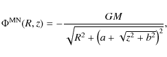
where M is the total mass and a and b are two parameters. It is useful to parametrize the Miyamoto-Nagai potential, introducing the horizontal scale length hR and the vertical scale length hzdefined by:
The potential then becomes:
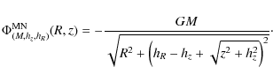
Using this parametrization, the circular velocity curve is written as:
![\begin{displaymath}v_{\rm {c}}^2 = R \frac{\partial}{\partial R}\Phi^{\rm {MN}}(R,0) =\frac{GMR^2}{\left[ R^2 + h_R^2 \right]^{3/2}},
\end{displaymath}](/articles/aa/full_html/2009/25/aa09883-08/img206.png)
which is independent of the vertical scale length hz. This means that any Miyamoto-Nagai model with mass M and horizontal scale length hR will fit the same rotation curve. One may also recognize in Eq. (A.4) the familiar velocity curve of the Plummer model, the latter being a subclass of the Miyamoto-Nagai model, with a=0and b=hR.
A corollary of Eq. (A.4) is that the rotation curve of any
Miyamoto-Nagai model can be reproduced by a linear combination of two
or more Miyamoto-Nagai models, having different scale heights and
appropriate masses. For example, the potential
![]() defined by
defined by
where
Appendix B: Evolution of model N = 3'
![\begin{figure}
\par\includegraphics[width=8.6cm,clip]{9883Fig20.eps}
\end{figure}](/articles/aa/full_html/2009/25/aa09883-08/img212.png) |
Figure B.1:
Evolution of model N=3' where the all the gas (visible and dark) is assumed to be dissipative. Each image represents the surface density of the visible gas. The box size is
|
| Open with DEXTER | |
In this appendix we present the evolution of model N=3', where all
the gas (visible and dark) is assumed to be dissipative, computed with
the sticky particle scheme (see Sect. 2.3). The
sticky parameters used are similar to the ones used for the visible gas
in model N=3 and N=5. The evolution shows that at the beginning
(
![]() )
the strongest dissipation reinforces the
spiral constant in the central part of the galaxy. But after
)
the strongest dissipation reinforces the
spiral constant in the central part of the galaxy. But after
![]() the inner disk, which is dynamically very cold, becomes
strongly unstable. The spirals break into several dense clumps and the
disk does not look like a real galaxy. This effect is even stronger
for an N=5 model, which is not displayed here. This test shows that
the dark matter in the disk cannot be as dissipative as the visible
disk. Otherwise, the disk is unstable and fragments in less than a
dynamical time.
the inner disk, which is dynamically very cold, becomes
strongly unstable. The spirals break into several dense clumps and the
disk does not look like a real galaxy. This effect is even stronger
for an N=5 model, which is not displayed here. This test shows that
the dark matter in the disk cannot be as dissipative as the visible
disk. Otherwise, the disk is unstable and fragments in less than a
dynamical time.
References
- Appleton, P. N., Xu, K. C., Reach, W., et al. 2006, ApJ, 639, L51 [NASA ADS] [CrossRef]
- Athanassoula, E. 1984, Phys. Rep., 114, 321 [NASA ADS] [CrossRef]
- Begum, A., Chengalur, J. N., Karachentsev, I. D., & Sharina, M. E. 2008, MNRAS, 386, 138 [NASA ADS] [CrossRef] (In the text)
- Binney, J., & Tremaine, S. 1987, Galactic dynamics (Princeton, NJ: Princeton University Press) (In the text)
- Bissantz, N., & Gerhard, O. 2002, MNRAS, 330, 591 [NASA ADS] [CrossRef] (In the text)
- Blais-Ouellette, S., Amram, P., & Carignan, C. 2001, AJ, 121, 1952 [NASA ADS] [CrossRef]
- Boomsma, R., Oosterloo, T. A., Fraternali, F., van der Hulst, J. M., & Sancisi, R. 2008, ArXiv e-prints, 807 (In the text)
- Bosma, A. 1978, Ph.D. Thesis, Groningen Univ.
- Bosma, A. 1981, AJ, 86, 1825 [NASA ADS] [CrossRef]
- Bottema, R. 2003, MNRAS, 344, 358 [NASA ADS] [CrossRef] (In the text)
- Boulanger, F., Maillard, J. P., Appleton, P., et al. 2008, Experimental Astronomy, 20 (In the text)
- Bournaud, F., & Combes, F. 2002, A&A, 392, 83 [NASA ADS] [CrossRef] [EDP Sciences]
- Bournaud, F., Duc, P.-A., Brinks, E., et al. 2007, Science, 316, 1166 [NASA ADS] [CrossRef] (In the text)
- Brahic, A. 1977, A&A, 54, 895 [NASA ADS]
- Broeils, A. H. 1992, Ph.D. Thesis, Univ. Groningen
- Bureau, M., Freeman, K. C., Pfitzner, D. W., & Meurer, G. R. 1999, AJ, 118, 2158 [NASA ADS] [CrossRef]
- Carignan, C., Charbonneau, P., Boulanger, F., & Viallefond, F. 1990, A&A, 234, 43 [NASA ADS]
- Cen, R., & Ostriker, J. P. 1999, ApJ, 514, 1 [NASA ADS] [CrossRef]
- Cen, R., & Ostriker, J. P. 2006, ApJ, 650, 560 [NASA ADS] [CrossRef]
- Combes, F., & Gerin, M. 1985, A&A, 150, 327 [NASA ADS]
- Combes, F., & Pfenniger, D. 1997, A&A, 327, 453 [NASA ADS] (In the text)
- Crosthwaite, L. P., Turner, J. L., Buchholz, L., Ho, P. T. P., & Martin, R. N. 2002, AJ, 123, 1892 [NASA ADS] [CrossRef] (In the text)
- Cuillandre, J.-C., Lequeux, J., Allen, R. J., Mellier, Y., & Bertin, E. 2001, ApJ, 554, 190 [NASA ADS] [CrossRef] (In the text)
- de Blok, W. J. G. 2005, ApJ, 634, 227 [CrossRef]
- de Blok, W. J. G., & Bosma, A. 2002, A&A, 385, 816 [NASA ADS] [CrossRef] [EDP Sciences]
- de Blok, W. J. G., & Walter, F. 2003, MNRAS, 341, L39 [NASA ADS] [CrossRef] (In the text)
- de Blok, W. J. G., Walter, F., Brinks, E., et al. 2008, AJ, 136, 2648 [NASA ADS] [CrossRef]
- Draine, B. T. 1978, ApJS, 36, 595 [NASA ADS] [CrossRef]
- Draine, B. T. 1998, ApJ, 509, L41 [NASA ADS] [CrossRef]
- Dubinski, J., Gauthier, J.-R., Widrow, L., & Nickerson, S. 2008, in ASP Conf. Ser. 396, ed. J. G. Funes & E. M. Corsini, 321
- Egami, E., Rieke, G. H., Fadda, D., & Hines, D. C. 2006, ApJ, 652, L21 [NASA ADS] [CrossRef] (In the text)
- Elmegreen, B. G. 1995, MNRAS, 275, 944 [NASA ADS] (In the text)
- Elmegreen, B. G. 1997, in New extragalactic perspectives in the new South Africa (Kluwer, 1996), 117, 467 (In the text)
- Ferguson, A. M. N., Wyse, R. F. G., Gallagher, J. S., & Hunter, D. A. 1998, ApJ, 506, L19 [NASA ADS] [CrossRef] (In the text)
- Font, A. S., Navarro, J. F., Stadel, J., & Quinn, T. 2001, ApJ, 563, L1 [NASA ADS] [CrossRef]
- Fukugita, M., & Peebles, P. J. E. 2004, ApJ, 616, 643 [NASA ADS] [CrossRef] (In the text)
- Fux, R. 2005, A&A, 430, 853 [NASA ADS] [CrossRef] [EDP Sciences]
- Gao, L., White, S. D. M., Jenkins, A., Stoehr, F., & Springel, V. 2004, MNRAS, 355, 819 [NASA ADS] [CrossRef] (In the text)
- Gauthier, J.-R., Dubinski, J., & Widrow, L. M. 2006, ApJ, 653, 1180 [NASA ADS] [CrossRef] (In the text)
- Gentile, G., Salucci, P., Klein, U., Vergani, D., & Kalberla, P. 2004, MNRAS, 351, 903 [NASA ADS] [CrossRef]
- Gentile, G., Burkert, A., Salucci, P., Klein, U., & Walter, F. 2005, ApJ, 634, L145 [NASA ADS] [CrossRef]
- Gerhard, O. 2006, in EAS Publications Series, ed. G. A. Mamon, F. Combes, C. Deffayet, & B. Fort, EAS Publ. Ser., 20, 89 (In the text)
- Gerhard, O., & Silk, J. 1996, ApJ, 472, 34 [NASA ADS] [CrossRef]
- Goldreich, P., & Lynden-Bell, D. 1965, MNRAS, 130, 125 [NASA ADS]
- Goldsmith, D. W., Habing, H. J., & Field, G. B. 1969, ApJ, 158, 173 [NASA ADS] [CrossRef] (In the text)
- Grenier, I. A., Casandjian, J.-M., & Terrier, R. 2005, Science, 307, 1292 [NASA ADS] [CrossRef] (In the text)
- Habing, H. J. 1968, Bull. Astron. Inst. Netherlands, 19, 421 [NASA ADS] (In the text)
- Harfst, S., Theis, C., & Hensler, G. 2006, A&A, 449, 509 [NASA ADS] [CrossRef] [EDP Sciences]
- Heithausen, A. 2002, A&A, 393, L41 [NASA ADS] [CrossRef] [EDP Sciences]
- Heithausen, A. 2004, ApJ, 606, L13 [NASA ADS] [CrossRef] (In the text)
- Henriksen, R. N., & Widrow, L. M. 1995, ApJ, 441, 70 [NASA ADS] [CrossRef]
- Hernquist, L. 1993, ApJS, 86, 389 [NASA ADS] [CrossRef] (In the text)
- Hoekstra, H., van Albada, T. S., & Sancisi, R. 2001, MNRAS, 323, 453 [NASA ADS] [CrossRef]
- Jiang, I.-G., & Binney, J. 1999, MNRAS, 303, L7 [NASA ADS] [CrossRef]
- Jog, C. J. 1996, MNRAS, 278, 209 [NASA ADS] (In the text)
- Jog, C. J., & Solomon, P. M. 1984a, ApJ, 276, 127 [NASA ADS] [CrossRef]
- Jog, C. J., & Solomon, P. M. 1984b, ApJ, 276, 114 [NASA ADS] [CrossRef]
- Johnston, K. V., Law, D. R., & Majewski, S. R. 2005, ApJ, 619, 800 [NASA ADS] [CrossRef] (In the text)
- Julian, W. H., & Toomre, A. 1966, ApJ, 146, 810 [NASA ADS] [CrossRef]
- Kalberla, P. M. W. 2003, ApJ, 588, 805 [NASA ADS] [CrossRef]
- Kalberla, P. M. W. 2004, Ap&SS, 289, 239 [NASA ADS] [CrossRef]
- Kalberla, P. M. W., & Kerp, J. 1998, A&A, 339, 745 [NASA ADS]
- Kalberla, P. M. W., Dedes, L., Kerp, J., & Haud, U. 2007, A&A, 469, 511 [NASA ADS] [CrossRef] [EDP Sciences]
- Katz, N., Weinberg, D. H., & Hernquist, L. 1996, ApJS, 105, 19 [NASA ADS] [CrossRef] (In the text)
- Kaufmann, T., Mayer, L., Wadsley, J., Stadel, J., & Moore, B. 2007, MNRAS, 375, 53 [NASA ADS] [CrossRef]
- Keres, D., Katz, N., Weinberg, D. H., & Davé, R. 2005, MNRAS, 363, 2 [NASA ADS] [CrossRef] (In the text)
- Kerins, E., Binney, J., & Silk, J. 2002, MNRAS, 332, L29 [NASA ADS] [CrossRef]
- Klypin, A., Kravtsov, A. V., Valenzuela, O., & Prada, F. 1999, ApJ, 522, 82 [NASA ADS] [CrossRef]
- Lelièvre, M., & Roy, J.-R. 2000, AJ, 120, 1306 [NASA ADS] [CrossRef] (In the text)
- Maio, U., Dolag, K., Ciardi, B., & Tornatore, L. 2007, MNRAS, 379, 963 [NASA ADS] [CrossRef] (In the text)
- Masset, F. S., & Bureau, M. 2003, ApJ, 586, 152 [NASA ADS] [CrossRef]
- Mayer, L., & Moore, B. 2004, MNRAS, 354, 477 [NASA ADS] [CrossRef] (In the text)
- Mayer, L., Governato, F., & Kaufmann, T. 2008, Adv. Sci. Lett., 1, 7 (In the text)
- Merlin, E., & Chiosi, C. 2007, A&A, 473, 733 [NASA ADS] [CrossRef] [EDP Sciences]
- Miyamoto, M., & Nagai, R. 1975, PASJ, 27, 533 [NASA ADS] (In the text)
- Moore, B., Ghigna, S., Governato, F., et al. 1999, ApJ, 524, L19 [NASA ADS] [CrossRef]
- Navarro, J. F., & Benz, W. 1991, ApJ, 380, 320 [NASA ADS] [CrossRef]
- Navarro, J. F., & Steinmetz, M. 1997, ApJ, 478, 13 [NASA ADS] [CrossRef]
- Ogle, P., Antonucci, R., Appleton, P. N., & Whysong, D. 2007, ApJ, 668, 699 [NASA ADS] [CrossRef]
- Papadopoulos, P. P., Thi, W.-F., & Viti, S. 2002, ApJ, 579, 270 [NASA ADS] [CrossRef] (In the text)
- Pfenniger, D. 2004, in Baryons in Dark Matter Halos, ed. R. Dettmar, U. Klein, & P. Salucci
- Pfenniger, D., & Combes, F. 1994, A&A, 285, 94 [NASA ADS] (In the text)
- Pfenniger, D., & Revaz, Y. 2005, A&A, 431, 511 [NASA ADS] [CrossRef] [EDP Sciences] (In the text)
- Pfenniger, D., Combes, F., & Martinet, L. 1994, A&A, 285, 79 [NASA ADS] (In the text)
- Reach, W. T., Franz, B. A., Weiland, J. L., et al. 1995, Nature, 374, 521 [NASA ADS] [CrossRef] (In the text)
- Reshetnikov, V., & Combes, F. 1999, A&AS, 138, 101 [NASA ADS] [CrossRef] [EDP Sciences]
- Revaz, Y., & Pfenniger, D. 2004, A&A, 425, 67 [NASA ADS] [CrossRef] [EDP Sciences] (In the text)
- Revaz, Y., & Pfenniger, D. 2007, a New Scenario for the Origin of Galacticwarps, Island Universes - Structure and Evolution of Disk Galaxies, 149 (In the text)
- Safa, Y., & Pfenniger, D. 2008, Eur. Phys. J. B, 66, 337 [NASA ADS] [CrossRef] [EDP Sciences] (In the text)
- Sánchez-Saavedra, M. L., Battaner, E., Guijarro, A., López-Corredoira, M., & Castro-Rodríguez, N. 2003, A&A, 399, 457 [NASA ADS] [CrossRef] [EDP Sciences]
- Schwarz, M. P. 1981, ApJ, 247, 77 [NASA ADS] [CrossRef]
- Seiden, P. E., Schulman, L. S., & Elmegreen, B. G. 1984, ApJ, 282, 95 [NASA ADS] [CrossRef] (In the text)
- Sellwood, J. A., & Binney, J. J. 2002, MNRAS, 336, 785 [NASA ADS] [CrossRef] (In the text)
- Semelin, B., & Combes, F. 2002, A&A, 388, 826 [NASA ADS] [CrossRef] [EDP Sciences]
- Shen, J., & Sellwood, J. A. 2006, MNRAS, 370, 2 [NASA ADS]
- Smith, D. A., Allen, R. J., Bohlin, R. C., Nicholson, N., & Stecher, T. P. 2000, ApJ, 538, 608 [NASA ADS] [CrossRef] (In the text)
- Spano, M., Marcelin, M., Amram, P., et al. 2008, MNRAS, 383, 297 [NASA ADS]
- Spekkens, K., Giovanelli, R., & Haynes, M. P. 2005, AJ, 129, 2119 [NASA ADS] [CrossRef]
- Springel, V. 2005, MNRAS, 364, 1105 [NASA ADS] [CrossRef] (In the text)
- Springel, V., Frenk, C. S., & White, S. D. M. 2006, Nature, 440, 1137 [NASA ADS] [CrossRef] (In the text)
- Strigari, L. E., Bullock, J. S., Kaplinghat, M., et al. 2007, ApJ, 669, 676 [NASA ADS] [CrossRef]
- Swaters, R. A., Madore, B. F., van den Bosch, F. C., & Balcells, M. 2003, ApJ, 583, 732 [NASA ADS] [CrossRef]
- Thilker, D. A., Bianchi, L., Boissier, S., et al. 2005, ApJ, 619, L79 [NASA ADS] [CrossRef] (In the text)
- Toomre, A. 1981, in Structure and Evolution of Normal Galaxies, ed. S. M. Fall, & D. Lynden-Bell, 111
- van den Bosch, F. C. 2001, MNRAS, 327, 1334 [NASA ADS] [CrossRef] (In the text)
- Walker, M., & Wardle, M. 1998, ApJ, 498, L125 [NASA ADS] [CrossRef]
- Wang, B., & Silk, J. 1994, ApJ, 427, 759 [NASA ADS] [CrossRef] (In the text)
- Watson, W. D. 1972, ApJ, 176, 103 [NASA ADS] [CrossRef]
- Weinberg, M. D., & Blitz, L. 2006, ApJ, 641, L33 [NASA ADS] [CrossRef]
Footnotes
- ... only
![[*]](/icons/foot_motif.png)
- The solution is the one of a two level transition system with
probabilities
 and
and
 .
.
- ...
momentum
- See Bournaud & Combes (2002) for details on the meaning of
 and
and
 .
.
- ... lines
- Here, a line is either a maximum or a minimum.
- ... Fig. 7)
- In fact the exact critical value may vary, depending on the
parameter
 and on the exact velocity curve through the
shear parameter
and on the exact velocity curve through the
shear parameter
 which
in our case is nearly equal to 1.
which
in our case is nearly equal to 1.
All Tables
Table 1: Multiphase model parameters.
Table 2: Parameters for the reference giant Sbc model.
Table 3: Parameters for the reference giant Sbc model.
All Figures
| |
Figure 1:
Schematic representation of the ISM two levels system. The visible gas is labeled VG, the dark gas DG and the stars ST. The probability of transition between the visible and the dark gas depends on the UV flux generated by young stars (
|
| Open with DEXTER | |
| In the text | |
| |
Figure 2:
Normalized UV flux |
| Open with DEXTER | |
| In the text | |
| |
Figure 3: Rotation curve of the reference model with the contribution of each component, the bulge, the exponential disk, the visible gas and the dark matter halo. |
| Open with DEXTER | |
| In the text | |
| |
Figure 4: Comparison of the surface density of baryons between model N=1 and model N=3. The total baryons (including stars) are traced in black. The red line represents the visible gas while the blue line (only present for the N=3 model) falling towards the center corresponds to the dark gas. |
| Open with DEXTER | |
| In the text | |
| |
Figure 5: Same figure as Fig. 4 but for model N=5. |
| Open with DEXTER | |
| In the text | |
| |
Figure 6: Comparison of the rotation curves of model N=1 and model N=3 and the contribution of each component. |
| Open with DEXTER | |
| In the text | |
| |
Figure 7: Same figure as Fig. 6 but for model N=5. |
| Open with DEXTER | |
| In the text | |
| |
Figure 8:
Model N=1+s: 100 |
| Open with DEXTER | |
| In the text | |
| |
Figure 9:
Comparison of the rotation curve of the 3 models at
|
| Open with DEXTER | |
| In the text | |
| |
Figure 10:
Surface density map of the stellar disk of the 3 models (N=1, N=3 and N=5, from left to right) at
|
| Open with DEXTER | |
| In the text | |
| |
Figure 11:
Comparison of the surface density of different components at
|
| Open with DEXTER | |
| In the text | |
| |
Figure 12:
Disk scale height as a function of the radius, for the four models at t=0.9 and
|
| Open with DEXTER | |
| In the text | |
| |
Figure 13:
Evolution of model N=1 between 0 and
|
| Open with DEXTER | |
| In the text | |
| |
Figure 14:
Evolution of model N=1 including 100 |
| Open with DEXTER | |
| In the text | |
| |
Figure 15:
Evolution of model N=3 between 0 and
|
| Open with DEXTER | |
| In the text | |
| |
Figure 16:
Evolution of model N=5 between 0 and
|
| Open with DEXTER | |
| In the text | |
| |
Figure 17:
Radial velocity dispersion at
|
| Open with DEXTER | |
| In the text | |
| |
Figure 18:
Stability of models N=1, N=3 and N=5 at different
times (0, 0.9, 1.8, 2.3, 3.2 and
|
| Open with DEXTER | |
| In the text | |
| |
Figure 19:
Evolution of the spiral structure in a ( |
| Open with DEXTER | |
| In the text | |
| |
Figure 20:
Evolution of the spiral structure in a ( |
| Open with DEXTER | |
| In the text | |
| |
Figure B.1:
Evolution of model N=3' where the all the gas (visible and dark) is assumed to be dissipative. Each image represents the surface density of the visible gas. The box size is
|
| Open with DEXTER | |
| In the text | |
Copyright ESO 2009
Current usage metrics show cumulative count of Article Views (full-text article views including HTML views, PDF and ePub downloads, according to the available data) and Abstracts Views on Vision4Press platform.
Data correspond to usage on the plateform after 2015. The current usage metrics is available 48-96 hours after online publication and is updated daily on week days.
Initial download of the metrics may take a while.