| Issue |
A&A
Volume 500, Number 3, June IV 2009
|
|
|---|---|---|
| Page(s) | 1027 - 1044 | |
| Section | Galactic structure, stellar clusters, and populations | |
| DOI | https://doi.org/10.1051/0004-6361/200811515 | |
| Published online | 01 April 2009 | |
The EROS2 search for microlensing events towards the spiral arms:
the complete seven season results![[*]](/icons/foot_motif.png) ,,
,,
Y. R. Rahal1,![]() -
C. Afonso2,
-
C. Afonso2,![]() -
J.-N. Albert1 -
J. Andersen3 -
R. Ansari1 - É. Aubourg2 -
P. Bareyre2 -
J.-P. Beaulieu4 -
X. Charlot2 -
F. Couchot1 -
C. Coutures2,4 -
F. Derue1,
-
J.-N. Albert1 -
J. Andersen3 -
R. Ansari1 - É. Aubourg2 -
P. Bareyre2 -
J.-P. Beaulieu4 -
X. Charlot2 -
F. Couchot1 -
C. Coutures2,4 -
F. Derue1,![]() -
R. Ferlet4 -
P. Fouqué7,8 -
J.-F. Glicenstein2 -
B. Goldman2,
-
R. Ferlet4 -
P. Fouqué7,8 -
J.-F. Glicenstein2 -
B. Goldman2,![]() -
A. Gould5 -
D. Graff5,
-
A. Gould5 -
D. Graff5,![]() -
M. Gros2 -
J. Haïssinski1 -
C. Hamadache2,
-
M. Gros2 -
J. Haïssinski1 -
C. Hamadache2,![]() -
J. de Kat2 -
É. Lesquoy2,4 -
C. Loup4 -
L. Le Guillou2,
-
J. de Kat2 -
É. Lesquoy2,4 -
C. Loup4 -
L. Le Guillou2,![]() -
C. Magneville 2 -
B. Mansoux 1 -
J.-B. Marquette4 -
É. Maurice6 -
A. Maury8,
-
C. Magneville 2 -
B. Mansoux 1 -
J.-B. Marquette4 -
É. Maurice6 -
A. Maury8,![]() -
A. Milsztajn 2,
-
A. Milsztajn 2,![]() -
M. Moniez1 -
N. Palanque-Delabrouille2 -
O. Perdereau1 -
S. Rahvar9 -
J. Rich2 -
M. Spiro2 -
P. Tisserand2,
-
M. Moniez1 -
N. Palanque-Delabrouille2 -
O. Perdereau1 -
S. Rahvar9 -
J. Rich2 -
M. Spiro2 -
P. Tisserand2,![]() -
A. Vidal-Madjar4
The EROS-2 collaboration
-
A. Vidal-Madjar4
The EROS-2 collaboration
1 - Laboratoire de l'Accélérateur Linéaire,
IN2 P3- CNRS, Université de Paris-Sud, BP 34, 91898 Orsay Cedex, France
2 -
CEA, DSM, DAPNIA,
Centre d'Études de Saclay, 91191 Gif-sur-Yvette Cedex, France
3 -
The Niels Bohr Institute, Astronomy Group, Juliane Maries vej 30,
2100 Copenhagen, Denmark
4 -
Institut d'Astrophysique de Paris, UMR 7095 CNRS, Université Pierre &
Marie Curie, 98 bis boulevard Arago, 75014 Paris, France
5 -
Department of Astronomy, Ohio State University, Columbus, Ohio 43210, USA
6 -
Observatoire de Marseille, INSU-CNRS,
2 place Le Verrier, 13248 Marseille Cedex 04, France
7 -
Observatoire Midi-Pyrénées, LATT, Université de Toulouse, CNRS,
14 Av. E. Belin, 31400 Toulouse, France
8 -
European Southern Observatory (ESO), Casilla 19001, Santiago 19, Chile
9 -
Dept. of Physics, Sharif University of Technology, Tehran, Iran
Received 12 December 2008 / Accepted 13 March 2009
Abstract
Aims. The EROS-2 project has been designed to search for microlensing events towards any dense stellar field. The densest parts of the Galactic spiral arms have been monitored to maximize the microlensing signal expected from the stars of the Galactic disk and bulge.
Methods. 12.9 million stars have been monitored during 7 seasons towards 4 directions in the Galactic plane, away from the Galactic center.
Results. A total of 27 microlensing event candidates have been found. Estimates of the optical depths from the 22 best events are provided. A first order interpretation shows that simple Galactic models with a standard disk and an elongated bulge are in agreement with our observations. We find that the average microlensing optical depth towards the complete EROS-cataloged stars of the spiral arms is
![]() ,
a number that is stable when the selection criteria are moderately varied. As the EROS catalog is almost complete up to IC=18.5, the optical depth estimated for the sub-sample of bright target stars with IC<18.5 (
,
a number that is stable when the selection criteria are moderately varied. As the EROS catalog is almost complete up to IC=18.5, the optical depth estimated for the sub-sample of bright target stars with IC<18.5 (
![]() )
is easier to interpret.
)
is easier to interpret.
Conclusions. The set of microlensing events that we have observed is consistent with a simple Galactic model. A more precise interpretation would require either a better knowledge of the distance distribution of the target stars, or a simulation based on a Galactic model. For this purpose, we define and discuss the concept of optical depth for a given catalog or for a limiting magnitude.
Key words: cosmology: dark matter - Galaxy: disk - Galaxy: bulge - Galaxy: structure - Galaxy: kinematics and dynamics - Galaxy: microlensing
1 Introduction
After the first reports of microlensing candidates (Aubourg et al. 1993; Alcock et al. 1993; Udalski et al. 1993), the EROS team has performed extensive microlensing surveys from 1996 to 2003, that monitored the Magellanic clouds and large regions in the Galactic plane. The EROS-2 search for lensing towards the Magellanic clouds (Tisserand et al. 2007) yielded significant upper limits on the fraction of the Milky Way halo that can be comprised of dark objects with masses between![\begin{displaymath}\tau/10^{-6}=(1.62 \pm 0.23)\exp[-a(\vert b\vert-3\hbox{$^\circ$ })] ,
\end{displaymath}](/articles/aa/full_html/2009/24/aa11515-08/img29.png)
with
 |
(2) |
This optical depth agrees with Galactic models (Evans & Belokurov 2002; Bissantz et al. 1997) and with the results of the MACHO (Popowski et al. 2005) and Ogle-II (Sumi et al. 2006) collaborations. The duration distribution of the events discovered by the three collaborations have been recently analyzed by Calchi Novati et al. 2008 to constrain the Galactic Bulge Initial Mass Function.
Our team has devoted about ![]() of the observing time during
7 seasons to the search for microlensing events towards
the Galactic Spiral Arms (GSA),
as far as 55 degrees in longitude away from the Galactic center.
In our previous publications (Derue et al. 1999, Derue et al. 2001, hereafter referred as
Papers I and II) describing the detection
of respectively 3 and 7 events, our attention was called on
a possible optical depth asymmetry, accompanied by an asymmetric event
dynamics with respect to the Galactic center. This marginal
effect (a
of the observing time during
7 seasons to the search for microlensing events towards
the Galactic Spiral Arms (GSA),
as far as 55 degrees in longitude away from the Galactic center.
In our previous publications (Derue et al. 1999, Derue et al. 2001, hereafter referred as
Papers I and II) describing the detection
of respectively 3 and 7 events, our attention was called on
a possible optical depth asymmetry, accompanied by an asymmetric event
dynamics with respect to the Galactic center. This marginal
effect (a ![]() probability to be accidental) could
be interpreted as an indication of a long Galactic bar within the bulge.
Its investigation required a
significant increase in the number of events.
probability to be accidental) could
be interpreted as an indication of a long Galactic bar within the bulge.
Its investigation required a
significant increase in the number of events.
In addition to the observing time increase (by more than a factor 2),
we improved our catalog of monitored stars by
increasing the limiting magnitude as well as by
recovering some fields and sub-fields that were not analyzed previously.
These improvements allowed us to recover another factor
![]() in
sensitivity.
Moreover the discrimination power for microlensing event identification
has been significantly improved, partly because
the light curves are longer and thus provide
a better rejection of recurrent variable objects.
in
sensitivity.
Moreover the discrimination power for microlensing event identification
has been significantly improved, partly because
the light curves are longer and thus provide
a better rejection of recurrent variable objects.
A specific difficulty in the analysis of the spiral arms survey
comes from the poor knownledge of the source distance distribution;
in contrast with the LMC, the SMC and the Galactic center red giant clump,
the monitored sources in the Galactic disk
span a wide range of distances (![]() kpc according to preliminary
studies, see Sect. 6.4.2).
Their mean distance is also uncertain and has been estimated to be
kpc according to preliminary
studies, see Sect. 6.4.2).
Their mean distance is also uncertain and has been estimated to be
![]() (Derue 1999).
We define in this paper
the notion of ``catalog optical depth'' (Sect. 9)
and provide all the necessary data to test Galactic models.
(Derue 1999).
We define in this paper
the notion of ``catalog optical depth'' (Sect. 9)
and provide all the necessary data to test Galactic models.
![\begin{figure}
\par\includegraphics[width=18cm]{1515f1.eps}
\end{figure}](/articles/aa/full_html/2009/24/aa11515-08/img36.png) |
Figure 1:
The Galactic plane fields (Galactic coordinates)
monitored by EROS superimposed on the image of the Milky-way.
The locations of our fields towards the spiral arms, as
well as our Galactic bulge fields (not discussed in this paper)
are shown.
The large blue dot towards
|
| Open with DEXTER | |
2 Microlensing basics
Gravitational microlensing (Paczynski 1986) occurs when a massive
compact object passes close enough to the line of sight of a star,
temporarily magnifying the received light.
In the approximation of a single point-like object acting as a
deflector on a single point-like source,
the total magnification of the source luminosity
at a given time t is the sum of the contributions of
two images, given by
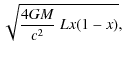
where u(t) is the distance of the deflecting object to the undeflected line of sight, expressed in units of the ``Einstein Radius''
| |
= |  |
(4) |
![$\displaystyle 4.54\ AU \times\left[\frac{M}{M_\odot}\right]^{\frac{1}{2}}
\time...
...}\right]^{\frac{1}{2}}
\times\frac{\left[x(1-x)\right]^{\frac{1}{2}}}{0.5}\cdot$](/articles/aa/full_html/2009/24/aa11515-08/img42.png) |
Here G is the Newtonian gravitational constant, L is the distance of the observer to the source and xL is its distance to the deflector of mass M. The motion of the deflector relative to the line of sight makes the magnification vary with time. Assuming a deflector moving at a constant relative transverse speed VT, reaching its minimum distance u0 (impact parameter) to the undeflected line of sight at time t0, u(t) is given by
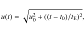
where
![$\displaystyle t_{\rm E} ({\rm days})=
79.\left[\frac{V_T}{100~ km/s}\right]^{-1...
...c{L}{10~~\rm kpc}\right]^{\frac{1}{2}}
\frac{[x(1-x)]^{\frac{1}{2}}}{0.5} \cdot$](/articles/aa/full_html/2009/24/aa11515-08/img45.png) |
(6) |
This simple microlensing description can be broken in many different ways: double lens (Mao & Stefano 1995), extended source, deviations from a uniform motion due either to the rotation of the Earth around the Sun (parallax effect) (Gould 1992; Hardy & Walker 1995), or to the orbital motion of the source around the center-of-mass of a multiple system, or to a similar motion of the deflector (see for example Möllerach & Roulet 2002).
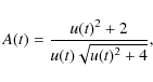
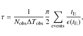
The optical depth ![]() towards a particular set of target stars
is defined as the
average probability for the line of sight to intercept
the Einstein disk of a deflector (magnification A > 1.34).
This probability is independent of the deflector mass function,
since the surface of the Einstein disk is proportional to
the deflector's mass.
When the target consists of a population of stars,
the measured optical depth is obtained from
towards a particular set of target stars
is defined as the
average probability for the line of sight to intercept
the Einstein disk of a deflector (magnification A > 1.34).
This probability is independent of the deflector mass function,
since the surface of the Einstein disk is proportional to
the deflector's mass.
When the target consists of a population of stars,
the measured optical depth is obtained from
 |
(7) |
where
 |
(8) |
3 Experimental setup and observations
The telescope, the camera and the observations, as well as the operations and data reduction are described in paper I and references therein. The star population locations and the amount of data collected towards the 29 fields that have been monitored in four different regions (Figure 2 shows the observation time span and the average sampling for the four different directions.
Table 1:
Characteristics of the 29 fields which were monitored
in the EROS spiral arm program:
locations of the field centers, average sampling
![]() (number of photometric measurements per light curve and per color)
and number of stars monitored for each field
(number of photometric measurements per light curve and per color)
and number of stars monitored for each field
![]() .
.
4 The catalogs
The catalogs of monitored stars have been produced following the procedure described in Papers I and II, based on the PEIDA photometric software (Ansari 1996). All objects are well identified in both colors and unambiguously associated between these two colors. We have removed objects that suffer from a strong contamination by a nearby bright star; the contribution to the background flux from such a nearby star at the position of the object should not exceed
The seven season data set contains 12.9 million objects measured
in the two colors:
3.0 towards
![]() ,
2.4 towards
,
2.4 towards
![]() ,
5.2 towards
,
5.2 towards
![]() and 2.3 towards
and 2.3 towards
![]() .
The number of monitored stars was increased by
.
The number of monitored stars was increased by
![]() since the
analysis of
Papers I and II, by producing a richer catalog from a wider choice of
good quality images than available before.
We were also able to solve some
technical problems that prevented us from producing the catalog for
some fields (Tisserand 2004; Rahal 2003).
The recovered stars are mainly faint stars
with a comparatively low
microlensing sensitivity.
since the
analysis of
Papers I and II, by producing a richer catalog from a wider choice of
good quality images than available before.
We were also able to solve some
technical problems that prevented us from producing the catalog for
some fields (Tisserand 2004; Rahal 2003).
The recovered stars are mainly faint stars
with a comparatively low
microlensing sensitivity.
4.1 Completeness, blending
We have compared a subset of the gs201 EROS field catalog (Fig. 3a) with the catalog extracted from the deeper HST-WFPC2 (Wide Field Planetary Camera 2) images (Fig. 3b) named U6FQ1102B (exposure 210 s with filter F606W) and U6FQ1104B (exposure 126 s with filter F814W), centered at ![\begin{figure}
\par\includegraphics[width=9.5cm]{1515f2.eps}
\end{figure}](/articles/aa/full_html/2009/24/aa11515-08/img74.png) |
Figure 2: Time sampling for each monitored direction: weekly average number of measurements per star since January 1rst, 1996. |
| Open with DEXTER | |
| |
Figure 3:
a) The
|
| Open with DEXTER | |

From the HST-EROS star association, we have extracted our
detection efficiencies as a function of the
![]() stellar magnitudes
(see Fig. 4).
stellar magnitudes
(see Fig. 4).
![\begin{figure}
\par\includegraphics[width=9.5cm]{1515f5.eps}
\end{figure}](/articles/aa/full_html/2009/24/aa11515-08/img79.png) |
Figure 4:
Top panel: the EROS (thick line) and HST (thin line)
|
| Open with DEXTER | |
4.2 The color-magnitude diagram
Figure 5 gives the color-magnitude diagramsWe were able to qualitatively reproduce these features with a (simple) simulated catalog, as explained below in Sect. 9.2 (Fig. 21). The color-magnitude diagram of this synthesized catalog shows two parallel features due to the main sequence and the red giant clump, that are similar to the ones observed in the data. Without spectroscopic data or a more detailed simulation, it is not possible to go further than this qualitative comparison for the interpretation of the observed color-magnitude diagrams.
4.3 Photometric precision
To complete the description of our observations, Fig. 6 gives the average point-to-point photometric dispersion along the light curves as a function of the magnitude IC.
![\begin{figure}
\par\includegraphics[width=18cm]{1515f6.eps}\par
\end{figure}](/articles/aa/full_html/2009/24/aa11515-08/img81.png) |
Figure 5:
Color-magnitude diagrams
|
| Open with DEXTER | |
5 The search for lensed stars
Our microlensing event detection scheme, based on light curve analysis, is the same as the one described in Papers I and II. The light curves for each star have been produced from the sequence of images using the software PEIDA (Ansari 1996); the mean numbers of photometric measurements per light curve are given for each monitored field in Table 1. In the following, we will outline the few specificities that arise because of analysis improvements, specific seasonal conditions or particular problems, and because of the fact that the time baseline is twice to three times longer than in our previous publications.
5.1 Prefiltering
We used the same non specific prefiltering described in Paper II, and preselected the most variable light curves satisfying at least one of the following criteria:
- the strongest fluctuation along the light curve (a series of consecutive flux measurements that lie below or above the ``base flux'', i.e. the average flux calculated in time regions devoid of significant fluctuations) has a small probability (typically smaller than 10-10) to happen for a stable star, assuming Gaussian errors;
- the dispersion of the flux measurements is significantly larger than expected from the photometric precision;
- the distribution of the deviations with respect to the base flux is incompatible with the distribution expected from the measurements of a stable source with Gaussian errors (using the Kolmogorov-Smirnov test).
5.2 Filtering
-
As in Paper II, we first searched
for bumps in each light curve.
A bump is defined as a series of consecutive flux measurements that starts
with a positive fluctuation of more than one
standard deviation (
 )
from the base flux,
ends when 3 consecutive measurements lie below
)
from the base flux,
ends when 3 consecutive measurements lie below  from the
base flux and contains at least four measurements deviating
by more than .
We characterize such a bump by
the parameter
from the
base flux and contains at least four measurements deviating
by more than .
We characterize such a bump by
the parameter
 where P is the probability
that the bump be due to an accidental occurrence
in a stable star light curve, assuming Gaussian errors.
We select the light curves whose most significant
fluctuation (bump 1) is positive in both colors;
where P is the probability
that the bump be due to an accidental occurrence
in a stable star light curve, assuming Gaussian errors.
We select the light curves whose most significant
fluctuation (bump 1) is positive in both colors;
-
then we require the time overlap between the main bumps
in each color to be at least
 of the combined time
intervals of the two bumps;
of the combined time
intervals of the two bumps;
- to reject most of the periodic or irregular variable stars, we remove those light curves that have a second bump (bump 2, positive or negative) with Q2>Q1/2 in one color.
5.3 Candidate selection
The observed flux versus time data
![]() is fitted with
the expression
is fitted with
the expression
![]() ,
where
,
where
![]() is the unmagnified flux and A(t)is given by expression (3).
The
is the unmagnified flux and A(t)is given by expression (3).
The ![]() per degree of freedom distribution of these three parameter fits for the 1097 light curves has a mean of 2.5 and a dispersion of 2.5.
The candidate selection is based on the fit quality (
per degree of freedom distribution of these three parameter fits for the 1097 light curves has a mean of 2.5 and a dispersion of 2.5.
The candidate selection is based on the fit quality (![]() )
and on
variables obtained from the
)
and on
variables obtained from the
![]() ,
t0,
,
t0, ![]() and u0fitted parameters.
We apply the following criteria,
tuned to select not only the ``simple'' microlensing events,
but also events that are affected by small deviations due to
parallax, source extension, binary lens effects... mentioned
in Sect. 2. The efficiency to detect caustics should be very
limited with this set of cuts, but none was found from a systematic
visual inspection of the 1097 light curves:
and u0fitted parameters.
We apply the following criteria,
tuned to select not only the ``simple'' microlensing events,
but also events that are affected by small deviations due to
parallax, source extension, binary lens effects... mentioned
in Sect. 2. The efficiency to detect caustics should be very
limited with this set of cuts, but none was found from a systematic
visual inspection of the 1097 light curves:
- C1. Minimum observation of the unmagnified epoch:
we first reduce the background due to instrumental effects
and to field crowding problems by selecting light curves that are sufficiently
sampled both during the unmagnified and the magnified stages.
For this purpose we define the ``high'' magnification epoch (called peak, labeled ``u<2'')
as the period of time during which the
fitted magnification A is above 1.06, associated to
an impact parameter u<2. The complementary ``low'' magnification epochs,
during which A<1.06, are labeled ``base''.
We require that

(10)
where is the
observation duration, and
is the
observation duration, and
 is the duration of the ``high'' magnification epoch;
- C2. Sampling during the magnified epoch:
we also require that the interval between the peak magnification time t0 and
the nearest measurement is smaller than
 ;
;
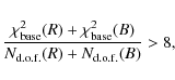
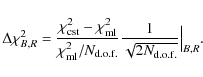
- C3. Goodness of a simple microlensing fit:
to ensure the fit quality,
we require
 separately for both colors,
where
separately for both colors,
where
 and the number of degrees of freedom
 are obtained from the full light curve;
- C4. Impact parameter: we also require that the fitted impact parameter u0 be less than 1 for both colors;
- C5. Stability of the unmagnified object:
one important feature of a microlensing light curve is its stability during the
low magnification epochs, except for the rare configurations of microlensed variable stars.
We reject light curves with
(11)
where the and
values correspond to the measurements
obtained during the low magnification epochs;
and
values correspond to the measurements
obtained during the low magnification epochs;
- C6. Improvement brought by the microlensing fit compared to a constant fit:
we use the same
 variables as in Paper II
to select light curves for which a simple microlensing fit is significantly
better than a constant value fit:
variables as in Paper II
to select light curves for which a simple microlensing fit is significantly
better than a constant value fit:
(12)
We select light curves with ;
;
- C7. Overlap in the two colors:
defining
 as the time interval during which the fitted magnification is
larger than 1.34 (u<1), we require a minimum overlap between the time
intervals found in the two colors:
as the time interval during which the fitted magnification is
larger than 1.34 (u<1), we require a minimum overlap between the time
intervals found in the two colors:
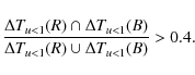
(13)
This loose requirement on the simultaneity of the magnifications in the two colors allows one to keep a good sensitivity to ``complex'' microlensing events; for example, this cut tolerates some difference between the fitted impact parameters obtained in the two colors (which may occur in the case of strong blending).
![\begin{figure}
\par\includegraphics[width=9.5cm]{1515f7.eps}
\end{figure}](/articles/aa/full_html/2009/24/aa11515-08/img106.png) |
Figure 6: Average photometric point-to-point precision along the light curves versus IC. The vertical bars show the dispersion of this precision in our source sample. The histogram shows the magnitude distribution of the full catalog (average over 4 directions). |
| Open with DEXTER | |
![\begin{figure}
\par\hspace*{4mm}\includegraphics[width=9cm,clip]{1515f8.eps}\vspace*{-5mm}
\hspace*{4mm}\includegraphics[width=9cm,clip]{1515f9.eps}
\end{figure}](/articles/aa/full_html/2009/24/aa11515-08/img107.png) |
Figure 7: Top panel: IC versus fitted u0 for the 27 microlensing candidates. Bottom panel: VJ-IC versus fitted u0. u0 is the fitted value assuming a point-like source and a point-like deflector with a constant speed. The red dots (respectively black dots) correspond to events with u0<0.7 used for optical depth studies (resp. 0.7<u0<1.). The small dots are the simulated events that satisfy the microlensing selection criteria. |
| Open with DEXTER | |
Table 2: Characteristics of the 27 microlensing candidates. For those events that have a better fit than the point-like point-source constant speed microlensing fit (the so-called standard fit), we also provide the standard fit parameters.
5.4 Non standard microlensing events
Some of our candidates are significantly better fitted with microlensing curves resulting from complex configurations than with the basic point-like source, point-like deflector with a constant-speed microlensing curve. The refinements that have been introduced in these cases are:
-
the blending of the lensed source with a nearby, unresolved object.
In that case, the light curve
 has to be fitted by
the following expression
has to be fitted by
the following expression
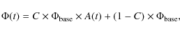
(14)
where C depends on the color. In supplement to the standard fit, this fit provides the CR and CB parameters, where C = (base flux of magnified component)/(total base flux). In the notes of Table 2, we give the magnitudes and colors of the microlensed components that take into account the color Eqs. (9); -
parallax.
Due to the rotation of the Earth around the Sun,
the apparent trajectory of the deflector with
respect to the line of sight is a cycloid instead of a straight line.
For some configurations (a nearby deflector and an event
that lasts a few months),
the resulting magnification versus time curve may be
affected by this parallax effect (Gould 1992, Hardy & Walker 1995).
The specific parameters that can
be fitted in this case are the Einstein radius
 and an orientation angle,
both projected on the observer's plane which is orthogonal
to the line of sight;
and an orientation angle,
both projected on the observer's plane which is orthogonal
to the line of sight;
-
``Xallarap''.
This effect is due to the rotation of the source around the center-of-mass
of a multiple system. In this case, the light curve exhibits modulations with
a characteristic time given by the period of the source rotation
(Derue et al. 1999; Möllerach & Roulet 2002).
Assuming a circular orbit,
the extra-parameters to be fitted or estimated are the orbital period P,
the luminosity ratio of the lensed object to the multiple system,
and the projected orbit radius in the deflector's plane
 ,
where a is the orbit radius and
,
where a is the orbit radius and
 .
.
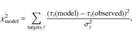
6 The microlensing candidates
6.1 General features
In order to quantify the relevance of the interpretation of the 27 selected objects as microlensing events, we define two variables as follows:
- ideally, the goodness of the microlensing fit should be uniform
throughout the observation duration.
Here we use fits made separately in the two colors.
Let
 and nu<2 be the microlensing fit
  and the number of degrees of freedom, restricted to the high magnification epoch
(
and the number of degrees of freedom, restricted to the high magnification epoch
(
 ,
see Sect. 5.3).
Let
and
,
see Sect. 5.3).
Let
and
 be the complementary
variables outside the peak period.
The variable
be the complementary
variables outside the peak period.
The variable
![$\displaystyle \delta_{fit}=
\left[\frac{\chi^2_{u<2}(R)+\chi^2_{u<2}(B)}{n_{u<2...
...i^2_{\rm base}(R)+\chi^2_{\rm base}(B)}{n_{\rm base}(R)+n_{\rm base}(B)}\right]$](/articles/aa/full_html/2009/24/aa11515-08/img131.png)
![$\displaystyle \times\left[\frac{1}{n_{u<2}(R)+n_{u<2}(B)}+\frac{1}{n_{\rm base}(R)+n_{\rm base}(B)}\right]^{-\frac{1}{2}}$](/articles/aa/full_html/2009/24/aa11515-08/img132.png)
(15)
quantifies the difference of the standard fit quality during and outside the microlensing peak, expressed in standard deviations (thanks to the second factor). A negative value of (<-5) is an indication of a non constant
base, and points to a variable star instead of a microlensing event.
For non-standard microlensing (parallax, blending...)
will be positive
and may be large (>10),
because the fit is expected to be less good in the peak than in the base;
(<-5) is an indication of a non constant
base, and points to a variable star instead of a microlensing event.
For non-standard microlensing (parallax, blending...)
will be positive
and may be large (>10),
because the fit is expected to be less good in the peak than in the base;
-
many of the EROS instrumental defects - such as bad pixels or
diffraction features - have a long lifetime, and last for entire
observing seasons. This produces long time scale false candidates.
A signal to noise indicator is provided by the ratio
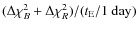 where
is defined above (criterion C6) and where
where
is defined above (criterion C6) and where
 characterizes the event time scale.
![\begin{figure}
\par\includegraphics[width=9.7cm]{1515f10.eps}
\end{figure}](/articles/aa/full_html/2009/24/aa11515-08/img135.png) |
Figure 8:
|
| Open with DEXTER | |
- a few (6) selected events have both a large positive
and
 .
These are events for which a non-standard microlensing fit provides a better interpretation.
Each of them is discussed in the remarks of Table 2;
.
These are events for which a non-standard microlensing fit provides a better interpretation.
Each of them is discussed in the remarks of Table 2;
- the bulk of our final sample (20) are events with a large
and
compatible with 0, as
expected for standard microlensing events (and as is the case for our simulated sample);
-
event GSA-u1 has a small
.
After visual inspection (see Appendix A, last event),
we cannot exclude a microlensing interpretation,
but the long duration and the lack of a reliable base
make it very uncertain, considering the relatively low value of
 (only 73.).
The status of this candidate remains pending until
further observations over a longer time range can be made.
One should keep in mind that confirmed events
of this type would give a major contribution to the optical depth
(GSAu1 would contribute for
(only 73.).
The status of this candidate remains pending until
further observations over a longer time range can be made.
One should keep in mind that confirmed events
of this type would give a major contribution to the optical depth
(GSAu1 would contribute for
 towards
 ).
).
6.2 Comparison with the EROS 3 year analysis (Paper II)
We first checked the coherence between the present results and those of Paper II. Three additional candidates (GSA8, 13 and 25) with a maximum occurring during the first three years have been found. GSA13 and GSA25 belong to subfields that were not analyzed in paper II. GSA8 is located at the border of two subfields, and was missed by our previous analysis that did not systematically explore the overlapping regions between subfields.
Four of the 7 candidates, all towards
![]() ,
found in Paper II
are now rejected for the following reasons:
,
found in Paper II
are now rejected for the following reasons:
- GSA4 and GSA7 both showed a second fluctuation after the first three years;
-
for GSA5, the
improvement when replacing a constant fit
by a microlensing fit is no longer significant enough, due to the low
signal to noise ratio that prevails for its
light curve during the 7 years of data taking;
-
GSA6 was found to have an impact parameter of
 in
Paper II. Taking
into account the full light curve, the new fitted value is
in
Paper II. Taking
into account the full light curve, the new fitted value is
 ,
now just above our threshold. Incidentally,
is also much
smaller than our threshold (60), indicating that the previous selection
of this event could have been due to a fluctuation.
,
now just above our threshold. Incidentally,
is also much
smaller than our threshold (60), indicating that the previous selection
of this event could have been due to a fluctuation.
6.3 Overlap with other published surveys
A very small region of
A small region of our survey
overlaps the MACHO fields (Thomas et al. 2005).
Amongst the 9 MACHO candidates or alerts found around
![]() ,
3 are located within one of our monitored fields, but have not been
selected in our analysis for the following reasons:
,
3 are located within one of our monitored fields, but have not been
selected in our analysis for the following reasons:
- MACHO alert number 302.44928.3523 is too faint to be measured in
 and no measurement was made in
 within 40 days of the
magnification maximum. Nevertheless, an object clearly appears in the
images around the maximum magnification date;
within 40 days of the
magnification maximum. Nevertheless, an object clearly appears in the
images around the maximum magnification date;
- MACHO alert number 301.45445.840 is too faint to be in the EROS catalog. Furthermore, EROS missed the event as its time of maximum magnification was 106 days before the first EROS observation of the corresponding field;
- MACHO alert number 302.45258.1038 was very close to one of the gaps located between CCDs. Thus many measurements are missing. Our standard procedure does not try to recover complete light curves in such a case, and the standard light curve failed our selection process. Nevertheless, we confirm the presence of the bump at the right time, with the maximum magnification occurring during the very first days of the EROS data taking.
6.4 Statistical properties of the candidate parameters
6.4.1 The lens configurations
Microlensing events occur with a flat-distributed impact parameter and minimum approach time. The sample of observed microlensing event (t0, u0) configurations should be statistically representative of such a distribution after taking into account our detection efficiencies. This is illustrated in Fig. 9, where simulated events are generated as described in Sect. 7.1.
![\begin{figure}
\par\includegraphics[width=9.7cm]{1515f11.eps}
\end{figure}](/articles/aa/full_html/2009/24/aa11515-08/img140.png) |
Figure 9: t0 versus fitted u0 for the simulated events satisfying the analysis criteria (small dots) and for the detected candidates (big dots). Red dots correspond to events with fitted u0<0.7 (``standard'' fit). In the case of complex events, the best fit u0 value is plotted. |
| Open with DEXTER | |
![\begin{figure}
\par\includegraphics[width=9.5cm]{1515f12.eps}\vspace*{-4mm}
\includegraphics[width=9.5cm]{1515f13.eps}
\end{figure}](/articles/aa/full_html/2009/24/aa11515-08/img141.png) |
Figure 10: Color-magnitude diagram and projections of the simulated events satisfying the analysis criteria (small dots) and the detected candidates (big dots). The arrows show ( VJ-IC,IC) of the magnified component in the case of blending (see notes of Table 2). The red dots represent those events that are used for the optical depth estimates. The histograms of these events are superimposed on the projections (not normalized). |
| Open with DEXTER | |
6.4.2 The microlensed star population
The microlensed star population should also be representative of
the monitored population weighted by the microlensing detection
efficiencies
and by the optical depth that may vary from source to source.
As the sources are likely to be distributed along the line of sight,
a possible variation of the optical depth with distance
must be considered in the data analysis.
As the light of a remote source is expected to be more reddened
than the light of a close one,
the optical depth ![]() should increase on
average with the color index.
Figure 10 shows our color-magnitude diagram,
weighted by the microlensing efficiencies and assuming the same
optical depth for all stars.
It is directly obtained from the simulated events
that satisfy the analysis requirements.
The distribution of the observed candidates is less
peaked than the simulated one in the low color index region
because the most reddened stars are more likely to be lensed.
We were able to qualitatively confirm this color bias
through the catalog produced with a simple simulation
towards
should increase on
average with the color index.
Figure 10 shows our color-magnitude diagram,
weighted by the microlensing efficiencies and assuming the same
optical depth for all stars.
It is directly obtained from the simulated events
that satisfy the analysis requirements.
The distribution of the observed candidates is less
peaked than the simulated one in the low color index region
because the most reddened stars are more likely to be lensed.
We were able to qualitatively confirm this color bias
through the catalog produced with a simple simulation
towards
![]() described in Sect. 9.2,
that takes into account the source distance distribution
(Fig. 11 left).
Figure 11(right) shows that the color distribution
of the lensed sources (obtained by weighting with the optical depth)
is significantly biased towards the red color with respect to the simulated
distribution of detected sources.
We conclude that the distance scattering of the sources can explain
the observed bias of the lensed stars towards red color.
A more complete interpretation will be provided in a forthcoming publication
accordingly to the guidelines given in Sect. 9.
described in Sect. 9.2,
that takes into account the source distance distribution
(Fig. 11 left).
Figure 11(right) shows that the color distribution
of the lensed sources (obtained by weighting with the optical depth)
is significantly biased towards the red color with respect to the simulated
distribution of detected sources.
We conclude that the distance scattering of the sources can explain
the observed bias of the lensed stars towards red color.
A more complete interpretation will be provided in a forthcoming publication
accordingly to the guidelines given in Sect. 9.
| |
Figure 11: Left: optical depth as a function of the distance (thick line), source distance distribution of a simulated catalog (thick histogram), and distance distribution weighted by the optical depth (thin histogram). Right: color distribution of the stars of the simulated catalog (thin line) and expected color distribution of the lensed stars (thick line). |
| Open with DEXTER | |
Two outliers need a specific comment. On closer inspection, it appears that GSA25 is a genuine microlensing candidate of a very faint star. It was detected because of the very strong magnification. This is a rare case, but there is no reason to discard it from our list. GSA19 is a very bright and very red object. It could be a strongly absorbed nearby star lensed by a closer object.
The spatial distribution of the candidates shown in Fig. 12 does not indicate any remarkable concentration.
6.5 Domain of sensitivity of the analysis
The C1 and C2 cuts that use the
![]() duration of the stage with magnification A>1.06mainly affect the light curves
which show long bumps. Removing these two cuts
adds 6 candidates, all of very long duration,
that have a poor signal to noise ratio.
As is the case for the GSA-u1 event, only a very long
monitoring could change the status of such candidates and
improve or degrade their signal to noise ratio.
Therefore one should keep in mind that the optical depths we
publish in this paper are almost insensitive to events
with
duration of the stage with magnification A>1.06mainly affect the light curves
which show long bumps. Removing these two cuts
adds 6 candidates, all of very long duration,
that have a poor signal to noise ratio.
As is the case for the GSA-u1 event, only a very long
monitoring could change the status of such candidates and
improve or degrade their signal to noise ratio.
Therefore one should keep in mind that the optical depths we
publish in this paper are almost insensitive to events
with
![]() (cf. the detection efficiency versus
(cf. the detection efficiency versus
![]() curve in Fig. 13).
curve in Fig. 13).
7 Optical depth
To obtain reliable optical depth values, we use a sub-sample
of good quality candidates which should be almost free of the microlensing
like variable objects that have been identified towards other EROS
targets (Tisserand et al. 2007; Hamadache et al. 2006) and in Sect. 6.2.
For this purpose, we will only keep those candidates that have u0<0.7in the fit that assumes a point-like source and a point-like deflector
with a constant speed. This is approximately equivalent to requesting
![]() .
Events GSA13, 14, 16, 24 and GSAu1 are then discarded for the optical depth
analysis.
.
Events GSA13, 14, 16, 24 and GSAu1 are then discarded for the optical depth
analysis.
7.1 Microlensing detection efficiency
We present here the efficiency calculation for the detection
of events with u0<0.7.
As for our previous papers, we calculate our detection efficiency
by superimposing simulated events on
measured light curves from an unbiased sub-sample of our catalog.
Events are simulated as point-source, point-lens constant velocity
microlensing events, with parameters uniformly spanning a domain
largely exceeding the domain of EROS sensitivity
(u0 up to 2,
![]() ,
t0 generated from 150 days
before the first observation to 150 days after the last).
Efficiency is defined as the ratio of events satisfying the selection
cuts to the number of events generated up to u0=1.
Figure 13 (upper left panel) shows the EROS efficiency
as a function of
the source position in the color-magnitude diagram
averaged over all the other parameters and over all directions.
The other frames of Fig. 13 show the
efficiency as a 2D-function of IC of the lensed star and
,
t0 generated from 150 days
before the first observation to 150 days after the last).
Efficiency is defined as the ratio of events satisfying the selection
cuts to the number of events generated up to u0=1.
Figure 13 (upper left panel) shows the EROS efficiency
as a function of
the source position in the color-magnitude diagram
averaged over all the other parameters and over all directions.
The other frames of Fig. 13 show the
efficiency as a 2D-function of IC of the lensed star and ![]() ,
and as a 1D-function of
,
and as a 1D-function of ![]() ,
u0, IC and VJ-IC,
averaged over all the other parameters, for each monitored direction.
The efficiency is significantly better towards
,
u0, IC and VJ-IC,
averaged over all the other parameters, for each monitored direction.
The efficiency is significantly better towards ![]() Nor, because
of the higher sampling of the light curves in this direction.
Nor, because
of the higher sampling of the light curves in this direction.
| |
Figure 12:
From left to right: spatial distribution
|
| Open with DEXTER | |
![\begin{figure}
\par\includegraphics[width=18cm,height=22cm]{1515f20.eps}
\end{figure}](/articles/aa/full_html/2009/24/aa11515-08/img148.png) |
Figure 13:
Microlensing detection efficiency.
Upper left: the efficiency in the (
VJ-IC, IC) plane
averaged over u0, t0, |
| Open with DEXTER | |
Table 3: Observed and predicted microlensing statistics.
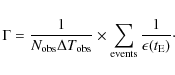
7.2 Optical depth determination
The optical depth values obtained from the 22 events that satisfy u0<0.7are given in the first part of Table 3.
The average over all directions is defined as
the proportion of stars covered by an Einstein disk. It is given by

where
 |
(16) |
following Han & Gould 1995. According to the discussion of Sect. 4.1, we assume a
7.3 Robustness of the optical depth values
We have studied the stability of the optical depth averaged over all fields by changing the selection cuts. Figure 14 gives the variation of ![\begin{figure}
\par\includegraphics[width=8.5cm]{1515f21c.eps}
\end{figure}](/articles/aa/full_html/2009/24/aa11515-08/img182.png) |
Figure 14:
Variation of the number of selected candidates (histogram, right scale)
and of
|
| Open with DEXTER | |
Figure 15 also gives
![]() as a function
of the u0 threshold. Our result does not depend on this cut
within statistical errors, showing that we probably found an
optimum between the quality of the events and the number of
those kept for our optical depth calculations.
as a function
of the u0 threshold. Our result does not depend on this cut
within statistical errors, showing that we probably found an
optimum between the quality of the events and the number of
those kept for our optical depth calculations.
![\begin{figure}
\includegraphics[width=8.5cm]{1515f22c.eps}
\end{figure}](/articles/aa/full_html/2009/24/aa11515-08/img183.png) |
Figure 15:
Variation of the number of selected candidates (histogram, right scale)
and of
|
| Open with DEXTER | |
Figures 16 and 17 show the variation of
![]() with the maximum magnitude Ic of the source population
and with the minimum color index VJ-IC.
There is no evidence for a variation with IC threshold.
As discussed below in Sect. 9.3,
this comes from the fact that the variation of
the optical depth with the distance does not result
in a variation with the magnitude as
more distant identified sources
do not appear fainter in our catalog on average.
Interestingly one may use these figures
to extract
with the maximum magnitude Ic of the source population
and with the minimum color index VJ-IC.
There is no evidence for a variation with IC threshold.
As discussed below in Sect. 9.3,
this comes from the fact that the variation of
the optical depth with the distance does not result
in a variation with the magnitude as
more distant identified sources
do not appear fainter in our catalog on average.
Interestingly one may use these figures
to extract ![]() for specific
stellar populations, in particular the
population of the brightest
stars with IC<18.5
that are better identified and measured, and that
suffer less blending (see Sect. 4.1).
for specific
stellar populations, in particular the
population of the brightest
stars with IC<18.5
that are better identified and measured, and that
suffer less blending (see Sect. 4.1).
![\begin{figure}
\par\includegraphics[width=8.5cm]{1515f23c.eps}
\end{figure}](/articles/aa/full_html/2009/24/aa11515-08/img184.png) |
Figure 16:
Number of selected candidates (histogram, right scale)
and
|
| Open with DEXTER | |
![\begin{figure}
\par\includegraphics[width=8.5cm]{1515f24c.eps}
\end{figure}](/articles/aa/full_html/2009/24/aa11515-08/img185.png) |
Figure 17:
Number of selected candidates (histogram, right scale)
and
|
| Open with DEXTER | |
8 Discussion: comparisons with simple models
8.1 Optical depth
We will consider here 4 published optical depth calculations and
our own calculations based on simple
Galactic models (model 1 without a thick disk, model 2 with a thick disk)
that we already used for discussions in Papers I and II.
The main revision to these 2 models since our previous
papers comes from the bulge inclination;
we now take
![]() instead of
instead of ![]() (Hamadache et al. 2006; and Picaud & Robin 2004)
as the angle of the outer bulge with respect
to the line of sight towards the Galactic center.
The only impact of this change is a little variation of our optical
depth value towards
(Hamadache et al. 2006; and Picaud & Robin 2004)
as the angle of the outer bulge with respect
to the line of sight towards the Galactic center.
The only impact of this change is a little variation of our optical
depth value towards
![]() .
We also completely
neglect any contribution from the halo to the optical
depth, in the light of the latest EROS results towards the Magellanic Clouds
(Tisserand et al. 2007).
As in our previous papers, we performed simple optical depth calculations
assuming all the sources to be at the same distance. More sophisticated
modelling based on the guidelines discussed in Sect. 9
will be considered in a forthcoming paper.
We give in Table 4 the list of the
geometrical and kinematical parameters used in these models I and II.
.
We also completely
neglect any contribution from the halo to the optical
depth, in the light of the latest EROS results towards the Magellanic Clouds
(Tisserand et al. 2007).
As in our previous papers, we performed simple optical depth calculations
assuming all the sources to be at the same distance. More sophisticated
modelling based on the guidelines discussed in Sect. 9
will be considered in a forthcoming paper.
We give in Table 4 the list of the
geometrical and kinematical parameters used in these models I and II.
Table 4: Parameters of the Galactic models 1 and 2 used in this article.
The disk densities are modeled by a double exponential expressed in cylindrical coordinates:
where
![\begin{eqnarray*}\rho_{B} &=& \frac{M_{B}}{6.57 \pi abc} {\rm e}^{-r^{2}/2} , \ ...
...t( \frac{y}{b} \right)^{2} \right]^{2} +
\frac{z^{4}}{c^{4}} ,
\end{eqnarray*}](/articles/aa/full_html/2009/24/aa11515-08/img209.png)
where MB is the bulge mass, and a, b, c the length scale factors. Figure 18 shows the measured optical depth as a function of the Galactic longitude, with the expectations from models 1 and 2 at
![\begin{figure}
\par\hspace*{3mm}\includegraphics[width=8.5cm]{1515f25.eps}
\end{figure}](/articles/aa/full_html/2009/24/aa11515-08/img212.png) |
Figure 18:
Expected optical depth up to
|
| Open with DEXTER | |
The optical depth predictions of model 1 and 2 and of the 4 following models are reported in Table 3:
-
Model A, from Binney et al. 1997, revised by Bissantz et al. 1997, has a
cuspy and flat Galatic bar, inclined by
 ;
;
-
Model B, described in Dwek et al. 1995, has a wider cuspy bar, inclined by
 ;
;
-
Model C, described in Freudenreich 1998, has a more
extended and diffuse bar, inclined by
 .
.
-
Model D, described in Grenacher et al. 1999, has a bar that is similar
to the one of our models 1 or 2, but inclined by
,
with a combination of a light thin disk plus a thick disk and a halo
contribution.
 |
(17) |
where
We cannot draw more conclusions about our model 1, as we know that it is not a realistic description, since all targets are supposed to be at the same distance. One may also notice that the extrapolation of any bulge model to the relatively distant region that we monitored is very uncertain. Nevertheless, it seems that ``heavy'' models trying to include a thick disk or any spiral structure are not favored. These results confirm the conclusions of Hamadache et al. (2006), in particular for model C, that is also disfavored by the present data.
8.2 Event duration distribution
Figure 19 gives the- the mass function for the lenses is taken from Gould, Bahcall & Flynn 1997 for both the disk and the bulge;
-
the solar motion with respect to the disk is taken from (Delhaye 1965):
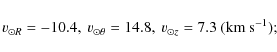
(18)
-
the global rotation of the disk is given by
![\begin{displaymath}V_{\rm rot}(r) = V_{\rm rot,\odot} \times \left[
1.00762 \left( \frac{r}{R_{\odot}} \right)^{0.0394} + 0.00712 \right] ,
\end{displaymath}](/articles/aa/full_html/2009/24/aa11515-08/img221.png)
(19)
where km s-1 (Brand & Blitz 1993);
- the peculiar velocity of disk stars is described by an anisotropic Gaussian distribution and a velocity dispersion given in Table 4;
-
the velocity distribution of the bulge stars is given by
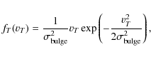
(20)
with .
.
![\begin{figure}
\par\includegraphics[width=9.5cm]{1515f26.eps}
\end{figure}](/articles/aa/full_html/2009/24/aa11515-08/img227.png) |
Figure 19:
Measured |
| Open with DEXTER | |
Table 3
gives the observed averages, dispersions and medians of
![]() ,
with the predictions from model 1 and models C and D.
Only mean duration predictions have been estimated for model C
(with no efficiency corrections)
and D (taking into account EROS microlensing detection efficiency).
The general tendency that emerges from the observations and that
is confirmed by the predictions
is that
,
with the predictions from model 1 and models C and D.
Only mean duration predictions have been estimated for model C
(with no efficiency corrections)
and D (taking into account EROS microlensing detection efficiency).
The general tendency that emerges from the observations and that
is confirmed by the predictions
is that
![]() increases with the Galactic longitude. This
is due to the fact that the direction of global motion of the lenses
tends to align with the line of sight when the longitude increases, and
consequently the transverse speed becomes smaller.
increases with the Galactic longitude. This
is due to the fact that the direction of global motion of the lenses
tends to align with the line of sight when the longitude increases, and
consequently the transverse speed becomes smaller.
As the variation of the microlensing detection
efficiency with ![]() is not taken into account in the predictions of
model C, we should compare here
the
is not taken into account in the predictions of
model C, we should compare here
the
![]() predicted values with the efficiency corrected means given by
predicted values with the efficiency corrected means given by
 |
(21) |
The observed corrected means are significantly larger than the predictions of model C with no spiral structure. This discrepancy could be explained (at least partially) by the absence of very short time scale events that have a negligible detection efficiency and can be totally missed in our statistically limited sample; a more precise comparison could be done between the observed
The mean durations predicted by Grenacher et al. (1999) (model D)
take into account the EROS efficiencies.
Therefore, we can directly compare the predictions
with our (uncorrected)
![]() values.
This model predicts longer durations than observed, but
here again it seems that the predictions
could be adjusted, as they are sensitive to the value of the minimal lens mass.
values.
This model predicts longer durations than observed, but
here again it seems that the predictions
could be adjusted, as they are sensitive to the value of the minimal lens mass.
9 Guidelines for further interpretation
As we always emphasized when presenting previous results towards the
spiral arms, the fact that the distance distribution of the target
sources is poorly known complicates the optical depth interpretation.
Figure 20 shows the expected optical depth as a function of the
Galactic longitude l, for different target distances, using model 1.
This figure shows first that the impact of the bulge
on the optical depth is significant only towards
![]() .
One also sees that the optical depth to distances smaller than
.
One also sees that the optical depth to distances smaller than
![]() is larger for l>0, the near side of the bulge,
because the number density of lenses is larger on this side;
but on the contrary, the OGLE II collaboration (Udalski et al. 2000a) reported
a larger rate for l<0 than for l>0in their catalog of microlensing events in the Galactic bulge.
This is due to the fact that
the optical depth averaged
over all distances can be larger for l<0, the far side of the bulge,
because there are more distant sources on this side, with a
larger optical depth. The observed asymmetry should then depend on the
selection of the monitored sources.
is larger for l>0, the near side of the bulge,
because the number density of lenses is larger on this side;
but on the contrary, the OGLE II collaboration (Udalski et al. 2000a) reported
a larger rate for l<0 than for l>0in their catalog of microlensing events in the Galactic bulge.
This is due to the fact that
the optical depth averaged
over all distances can be larger for l<0, the far side of the bulge,
because there are more distant sources on this side, with a
larger optical depth. The observed asymmetry should then depend on the
selection of the monitored sources.
![\begin{figure}
\par\hspace*{3mm}\includegraphics[width=8.5cm]{1515f27.eps}
\end{figure}](/articles/aa/full_html/2009/24/aa11515-08/img231.png) |
Figure 20:
Model 1 predictions for the optical depth at
6, 7, 8, 9, 10, 11 and 12 kpc (from lowest to highest curve)
at a Galactic latitude
|
| Open with DEXTER | |
9.1 The concept of ``catalog optical depth''
The EROS measured optical depth is
the average over the distance distribution
of the monitored sources.
Establishing this distance distribution
through individual spectrophotometric
measurements would require an enormous amount of complementary observations.
This leads us to define the concept of ``catalog optical depth''
![]() ,
which is relative to a particular catalog of monitored stars:
,
which is relative to a particular catalog of monitored stars:
![]() is
defined as the fraction of stars of a given catalog that undergo a
magnification A>1.34.
Our measured optical depth can be compared with
the depth derived from a lens and source distribution model
as follows:
first, one has to generate a synthetic source catalog
that matches our own catalog, taking into account
the EROS star detection efficiency (Fig. 4);
then one can use the generated source distance distribution
to estimate the average optical depth and compare it with the
measurements. This procedure is described in more detail below.
is
defined as the fraction of stars of a given catalog that undergo a
magnification A>1.34.
Our measured optical depth can be compared with
the depth derived from a lens and source distribution model
as follows:
first, one has to generate a synthetic source catalog
that matches our own catalog, taking into account
the EROS star detection efficiency (Fig. 4);
then one can use the generated source distance distribution
to estimate the average optical depth and compare it with the
measurements. This procedure is described in more detail below.
9.2 Synthesizing a catalog that matches the EROS one
Let
![]() be the source number density
predicted by the model
as a function of the distance D and of the absolute magnitude MIand color MV-MI;
let AI(D) and AV(D) be the predicted absorptions in I and V.
The pre-requisite for an optical depth interpretation is that
be the source number density
predicted by the model
as a function of the distance D and of the absolute magnitude MIand color MV-MI;
let AI(D) and AV(D) be the predicted absorptions in I and V.
The pre-requisite for an optical depth interpretation is that
![]() ,
the density per solid angle per apparent magnitude and color index
of the synthesized source catalog, fits the observed one
within the visible color-magnitude diagram.
This density is related to
,
the density per solid angle per apparent magnitude and color index
of the synthesized source catalog, fits the observed one
within the visible color-magnitude diagram.
This density is related to
![]() as follows:
as follows:
 |
(22) |
where
For the comparison with the observations,
the color-magnitude diagrams
![]() of our
catalogs (Fig. 5)
should be used.
They provide the observed stellar density per unit solid angle
in the effectively monitored field, that is corrected for
the dead regions of our CCDs, the overlap between fields and
the blind regions around the brightest objects.
of our
catalogs (Fig. 5)
should be used.
They provide the observed stellar density per unit solid angle
in the effectively monitored field, that is corrected for
the dead regions of our CCDs, the overlap between fields and
the blind regions around the brightest objects.
We show here the color-magnitude diagram of a preliminary catalog obtained with this procedure (Fig. 21). This catalog has been produced for the qualitative understanding of the observed diagrams (Sect. 4.2, Fig. 5) and also of the color bias of the lensed population (Sect. 6.4.2, Fig. 11).
![\begin{figure}
\par\includegraphics[width=8.5cm]{1515f28.eps}
\end{figure}](/articles/aa/full_html/2009/24/aa11515-08/img239.png) |
Figure 21:
Simulated color-magnitude diagram towards
|
| Open with DEXTER | |
| (24) |
where
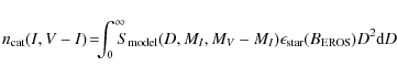
9.3 Estimating the average optical depth
Once the synthesis of a catalog is performed, one can compute the average optical depth over the synthesized catalog: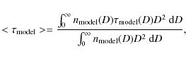 |
(25) |
where
| (26) |
is the number density of stars (per solid angle and distance unit) located at distance D that enters the catalog.
This procedure assumes that the average microlensing detection efficiency does not vary significantly with the distance of the sources. This is indeed the case because both the efficiency of our star detector and the average microlensing detection efficiency depend on the apparent magnitudes. The microlensing detection efficiency averaged on distant detected stellar populations is then similar to the one averaged on nearby detected populations because their apparent magnitude distributions are both peaked around the limiting magnitude. We have checked these features with simulations using our star detection efficiencies.
The observed optical depths in Table 3 are relative
to our entire catalogs. We recall here the average value for the 4 targets
(
![]() stars):
stars):

For easier comparisons, we extract from Fig. 16 the following optical depth

relative to the sub-set of 6.52 million stars brighter than Ic=18.5, for which our catalog is close to being complete.
10 Conclusions
The microlensing event search of EROS2 towards transparent windows of
the spiral arms leads to
optical depths that are consistent with a very simple Galactic model.
The possibility of a long bar that was proposed
in our paper II as a possible explanation of the observed optical depth
and duration asymetries is not confirmed; indeed, the inclination of the bar
was revised since the time of this publication, and the final optical
depth measured towards
![]() is also smaller (but statistically compatible).
A more complete interpretation that would take into account the distance distribution
of the monitored sources needs a model that allows one to synthesize
the EROS catalogs of these sources.
With such a model, one would also be able to make use of the
event duration distributions.
is also smaller (but statistically compatible).
A more complete interpretation that would take into account the distance distribution
of the monitored sources needs a model that allows one to synthesize
the EROS catalogs of these sources.
With such a model, one would also be able to make use of the
event duration distributions.
The VISTA project with its wide field infrared camera appears to offer an excellent opportunity to improve our knowledge of the microlensing towards the Galactic plane. The infrared light will allow the observers to monitor stars through dust, making them free of the transparent windows that were limiting the EROS fields.
Acknowledgements
We are grateful to the technical staff at ESO, La Silla for the support given to the EROS-2 project. We thank J-F. Lecointe and A. Gomes for the assistance with the online computing and the staff of the CC-IN2P3, especially the team in charge of the HPSS storage system, for their help with the data management.
References
- Afonso, C., Albert, J.-N., Andersen, J., et al. ( EROS Coll.) 2003, A&A, 400, 951 (In the text)
- Alcock, C., Akerlof, C. W., Allsman, R. A., et al. ( MACHO Coll.) 1993, Nature, 365, 621 (In the text)
- Alcock, C., Allsman, R. A., Alves, D., et al., 2000, ApJ, 542, 281 [NASA ADS] [CrossRef] (In the text)
- Ansari, R. 1996, Vistas in Astronomy, 40, 4 [CrossRef] (In the text)
- Aubourg, É., Bareyre, P., Bréhin, S., et al. ( EROS Coll.) 1993, Nature, 365, 623 (In the text)
- Bennett, D. P. 2005, ApJ, 633, 906 [NASA ADS] [CrossRef] (In the text)
- Binney, J., Gerhard, O., & Spergel, D. 1997, MNRAS, 288, 365 [NASA ADS] (In the text)
- Bissantz, N., & Gerhard, O. 2002, MNRAS, 330, 591 [NASA ADS] [CrossRef]
- Bissantz, N., Englmaier, P., Binney, J., & Gerhard, O. 1997, MNRAS, 289, 651 [NASA ADS] (In the text)
- Brand, J., & Blitz, L. 1993, A&A, 275, 67 [NASA ADS] (In the text)
- Calchi Novati, S., De Luca, F., Jetzer, Ph., et al. 2008, A&A, 480, 723 [NASA ADS] [CrossRef] [EDP Sciences] (In the text)
- Derue, F., Afonso, C., Alard, C., et al. ( EROS Coll.) 1999, A&A, 351, 87 (In the text)
- Derue, F. 1999, Ph.D. Thesis, CNRS/IN2 P3, LAL report 99-14, Université Paris 11 (In the text)
- Derue, F., Afonso, C., Alard, C., et al. ( EROS Coll.) 2001, A&A, 373, 126 (In the text)
- Delhaye, J. 1965, in Galactic Structure, The University of Chicago Press (In the text)
- Dwek, E., Arendt, R. G., Hauser, M. G., et al. 1995, ApJ, 445, 716 [NASA ADS] [CrossRef] (In the text)
- Epchtein, N., Deul, E., Derriere, S., et al. 1999, A&A, 349, 236 [NASA ADS] (In the text)
- Evans, N. W., & Belokurov, V. 2002, ApJ, 567, L119 [NASA ADS] [CrossRef] (In the text)
- Feldman, G. J., & Cousins, R. D. 1998, Phys. Rev. D, 57, 3873 [NASA ADS] [CrossRef] (In the text)
- Freudenreich, H. T. 1998, ApJ, 492, 495 [NASA ADS] [CrossRef] (In the text)
- Gould, A. 1992, ApJ, 392, 442 [NASA ADS] [CrossRef] (In the text)
- Gould, A., Bahcall, J. N., & Flynn, C. 1997, ApJ, 482, 913 [NASA ADS] [CrossRef] (In the text)
- Grenacher, L., Jetzer, P., Straässle, M., & de Paolis, F. 1999, A&A, 351, 775 [NASA ADS] (In the text)
- Hamadache, C., Le Guillou, L., Tisserand, P., et al. 2006, A&A, 454, 185 [NASA ADS] [CrossRef] [EDP Sciences] (In the text)
- Han, C., & Gould, A. 1995, ApJ, 449, 521 [NASA ADS] [CrossRef] (In the text)
- Hardy, S. J., & Walker, M. A. 1995, MNRAS, 276, L79 [NASA ADS] (In the text)
- The Hipparcos and Tycho Catalogs, ed. M. A. C. Perryman (SP-1200; Noordwijk: ESA) (In the text)
- HST archive, http://archive.stsci.edu/ (In the text)
- Mao, S., & Stefano, R. D. 1995, ApJ, 440, 22 [NASA ADS] [CrossRef] (In the text)
- Möllerach, S., & Roulet, E. 2002, Gravitational lensing and microlensing (World Scientific) (In the text)
- OGLE web page: http://www.astrouw.edu.pl/ogle/ogle2/fields.html (In the text)
- Paczynski, B. 1986, ApJ, 304, 1 [NASA ADS] [CrossRef] (In the text)
- Picaud, S., & Robin, A. C. 2004, A&A, 428, 891 [NASA ADS] [CrossRef] [EDP Sciences] (In the text)
- Popowski, P., Griest, K., Thomas, C. L., et al. 2005, ApJ, 631, 879 [NASA ADS] [CrossRef] (In the text)
- Rahal, Y. R. 2003, Ph.D. Thesis, Université Paris 6, LAL-CNRS/IN2 P3 report 03-85 (In the text)
- Rahvar, S. 2004, MNRAS, 347, 213 [NASA ADS] [CrossRef] (In the text)
- Sumi, T., Wozniak, P. R., Udalski, A., et al. (OGLE coll.) 2006, ApJ, 636, 240 (In the text)
- Tisserand, P. 2004, Ph.D. Thesis, Université de Nice-Sophya Antipolis CEA DAPNIA-04-09-T (In the text)
- Tisserand, P., Le Guillou, L., Afonso, C., et al. 2007, A&A, 469, 387 [NASA ADS] [CrossRef] [EDP Sciences] (In the text)
- Thomas, C. L., Griest, K., Popowski, P., et al. 2005, ApJ, 631, 906 [NASA ADS] [CrossRef] (In the text)
- Turon, C., Réquième, Y., Grenon, M., et al. 1995, A&A, 304, 82 [NASA ADS] (In the text)
- Udalski, A., Szymanski, M., Kaluzny, J., et al. ( OGLE Coll.) 1993, Act. Astr., 43, 289 (In the text)
- Udalski, A., Zebrun, K., Szymanski, M., et al. 2000a, Acta. Astr. 50, 1 (In the text)
- Udalski, A., Szymanski, M., Kubiak, M., et al. 2000b, Acta. Astr. 50, 307 (In the text)
- Weingartner, J. C., & Draine, B. T. 2001, ApJ, 548, 296 [NASA ADS] [CrossRef] (In the text)
Online Material
Appendix A: Light curves and finding charts of the microlensing candidates
![\begin{figure}\par\includegraphics[width=17cm,clip]{f22.eps}\par
\end{figure}](/articles/aa/full_html/2009/24/aa11515-08/img250.png) |
Figure A.1:
Finding charts (
|
| Open with DEXTER | |
![\begin{figure}\par\includegraphics[width=17cm,clip]{f23.eps}\end{figure}](/articles/aa/full_html/2009/24/aa11515-08/img251.png) |
Figure A.2: Light curves and finding charts (continued). |
| Open with DEXTER | |
![\begin{figure}\includegraphics[width=17cm,clip]{f24.eps}\end{figure}](/articles/aa/full_html/2009/24/aa11515-08/img252.png) |
Figure A.3: Light curves and finding charts (continued). |
| Open with DEXTER | |
![\begin{figure}\includegraphics[width=17cm,clip]{f25.eps}\end{figure}](/articles/aa/full_html/2009/24/aa11515-08/img253.png) |
Figure A.4: Light curves and finding charts (continued). |
| Open with DEXTER | |
Footnotes
- ... results
- See also our WWW server at URL: http://eros.in2p3.fr
- ...
- Color-magnitude tables of the EROS catalogs (Fig. 5) in ascii are available in electronic form at the CDS via anonymous ftp to cdsarc.u-strasbg.fr (130.79.128.5) or via http://cdsweb.u-strasbg.fr/cgi-bin/qcat?J/A+A/500/1027
- ...
- Figures of Appendix A are only available in electronic form at http://www.aanda.org
- ...
- Now at Electronics Arts Canada, Vancouver, Canada.
- ...
- Now at Max-Planck-Institut für Astronomie, Koenigstuhl 17, 69117 Heidelberg, Germany.
- ...
- Now at LPNHE, 4 place Jussieu, 75252 Paris Cedex 5, France.
- ...
- Now at Max-Planck-Institut für Astronomie, Koenigstuhl 17, 69117 Heidelberg, Germany.
- ...
- Now at Division of Medical Imaging Physics, Johns Hopkins University Baltimore, MD 21287-0859, USA.
- ...
- Also at CSNSM, Université Paris Sud 11, IN2P3-CNRS, 91405 Orsay Campus, France.
- ...
- Now at LPNHE, 4 place Jussieu, 75252 Paris Cedex 5, France.
- ...
- Now at San Pedro de Atacama Celestial Exploration, Casilla 21, San Pedro de Atacama, Chile.
- ...
- Deceased.
- ...
- Now at Mount Stromlo Observatory, Weston PO, ACT, 2611, Australia.
All Tables
Table 1:
Characteristics of the 29 fields which were monitored
in the EROS spiral arm program:
locations of the field centers, average sampling
![]() (number of photometric measurements per light curve and per color)
and number of stars monitored for each field
(number of photometric measurements per light curve and per color)
and number of stars monitored for each field
![]() .
.
Table 2: Characteristics of the 27 microlensing candidates. For those events that have a better fit than the point-like point-source constant speed microlensing fit (the so-called standard fit), we also provide the standard fit parameters.
Table 3: Observed and predicted microlensing statistics.
Table 4: Parameters of the Galactic models 1 and 2 used in this article.
All Figures
| |
Figure 1:
The Galactic plane fields (Galactic coordinates)
monitored by EROS superimposed on the image of the Milky-way.
The locations of our fields towards the spiral arms, as
well as our Galactic bulge fields (not discussed in this paper)
are shown.
The large blue dot towards
|
| Open with DEXTER | |
| In the text | |
| |
Figure 2: Time sampling for each monitored direction: weekly average number of measurements per star since January 1rst, 1996. |
| Open with DEXTER | |
| In the text | |
| |
Figure 3:
a) The
|
| Open with DEXTER | |
| In the text | |
| |
Figure 4:
Top panel: the EROS (thick line) and HST (thin line)
|
| Open with DEXTER | |
| In the text | |
| |
Figure 5:
Color-magnitude diagrams
|
| Open with DEXTER | |
| In the text | |
| |
Figure 6: Average photometric point-to-point precision along the light curves versus IC. The vertical bars show the dispersion of this precision in our source sample. The histogram shows the magnitude distribution of the full catalog (average over 4 directions). |
| Open with DEXTER | |
| In the text | |
| |
Figure 7: Top panel: IC versus fitted u0 for the 27 microlensing candidates. Bottom panel: VJ-IC versus fitted u0. u0 is the fitted value assuming a point-like source and a point-like deflector with a constant speed. The red dots (respectively black dots) correspond to events with u0<0.7 used for optical depth studies (resp. 0.7<u0<1.). The small dots are the simulated events that satisfy the microlensing selection criteria. |
| Open with DEXTER | |
| In the text | |
| |
Figure 8:
|
| Open with DEXTER | |
| In the text | |
| |
Figure 9: t0 versus fitted u0 for the simulated events satisfying the analysis criteria (small dots) and for the detected candidates (big dots). Red dots correspond to events with fitted u0<0.7 (``standard'' fit). In the case of complex events, the best fit u0 value is plotted. |
| Open with DEXTER | |
| In the text | |
| |
Figure 10: Color-magnitude diagram and projections of the simulated events satisfying the analysis criteria (small dots) and the detected candidates (big dots). The arrows show ( VJ-IC,IC) of the magnified component in the case of blending (see notes of Table 2). The red dots represent those events that are used for the optical depth estimates. The histograms of these events are superimposed on the projections (not normalized). |
| Open with DEXTER | |
| In the text | |
| |
Figure 11: Left: optical depth as a function of the distance (thick line), source distance distribution of a simulated catalog (thick histogram), and distance distribution weighted by the optical depth (thin histogram). Right: color distribution of the stars of the simulated catalog (thin line) and expected color distribution of the lensed stars (thick line). |
| Open with DEXTER | |
| In the text | |
| |
Figure 12:
From left to right: spatial distribution
|
| Open with DEXTER | |
| In the text | |
| |
Figure 13:
Microlensing detection efficiency.
Upper left: the efficiency in the (
VJ-IC, IC) plane
averaged over u0, t0, |
| Open with DEXTER | |
| In the text | |
| |
Figure 14:
Variation of the number of selected candidates (histogram, right scale)
and of
|
| Open with DEXTER | |
| In the text | |
| |
Figure 15:
Variation of the number of selected candidates (histogram, right scale)
and of
|
| Open with DEXTER | |
| In the text | |
| |
Figure 16:
Number of selected candidates (histogram, right scale)
and
|
| Open with DEXTER | |
| In the text | |
| |
Figure 17:
Number of selected candidates (histogram, right scale)
and
|
| Open with DEXTER | |
| In the text | |
| |
Figure 18:
Expected optical depth up to
|
| Open with DEXTER | |
| In the text | |
| |
Figure 19:
Measured |
| Open with DEXTER | |
| In the text | |
| |
Figure 20:
Model 1 predictions for the optical depth at
6, 7, 8, 9, 10, 11 and 12 kpc (from lowest to highest curve)
at a Galactic latitude
|
| Open with DEXTER | |
| In the text | |
| |
Figure 21:
Simulated color-magnitude diagram towards
|
| Open with DEXTER | |
| In the text | |
| |
Figure A.1:
Finding charts (
|
| Open with DEXTER | |
| In the text | |
| |
Figure A.2: Light curves and finding charts (continued). |
| Open with DEXTER | |
| In the text | |
| |
Figure A.3: Light curves and finding charts (continued). |
| Open with DEXTER | |
| In the text | |
| |
Figure A.4: Light curves and finding charts (continued). |
| Open with DEXTER | |
| In the text | |
Copyright ESO 2009
Current usage metrics show cumulative count of Article Views (full-text article views including HTML views, PDF and ePub downloads, according to the available data) and Abstracts Views on Vision4Press platform.
Data correspond to usage on the plateform after 2015. The current usage metrics is available 48-96 hours after online publication and is updated daily on week days.
Initial download of the metrics may take a while.