Photometric redshifts for the CFHTLS T0004 deep and wide fields

J. Coupon; O. Ilbert; M. Kilbinger; H. J. McCracken; Y. Mellier; S. Arnouts; E. Bertin; P. Hudelot; M. Schultheis; O. Le Fèvre; V. Le Brun; L. Guzzo; S. Bardelli; E. Zucca; M. Bolzonella; B. Garilli; G. Zamorani; A. Zanichelli; L. Tresse; H. Aussel

doi:10.1051/0004-6361/200811413

Home

All issues

Volume 500 / No 3 (June IV 2009)

A&A, 500 3 (2009) 981-998

Full HTML

Free Access

Issue		A&A Volume 500, Number 3, June IV 2009


Page(s)		981 - 998
Section		Cosmology (including clusters of galaxies)
DOI		https://doi.org/10.1051/0004-6361/200811413
Published online		29 April 2009

Photometric redshifts for the CFHTLS T0004 deep and wide fields

J. Coupon¹ - O. Ilbert² - M. Kilbinger¹ - H. J. McCracken¹ - Y. Mellier¹ - S. Arnouts³ - E. Bertin¹ - P. Hudelot¹ - M. Schultheis⁴ - O. Le Fèvre⁵ - V. Le Brun⁵ - L. Guzzo⁶ - S. Bardelli⁷ - E. Zucca⁷ - M. Bolzonella⁷ - B. Garilli⁶ - G. Zamorani⁷ - A. Zanichelli⁸ - L. Tresse⁵ - H. Aussel⁹

1 - Institut d'Astrophysique de Paris, UMR 7095 CNRS, Université Pierre et Marie Curie, 98bis boulevard Arago, 75014 Paris, France
2 - Institute for Astronomy, 2680 Woodlawn Dr., University of Hawaii, Honolulu, Hawaii, 96822, USA
3 - Canada-France-Hawaii telescope, 65-1238 Mamalahoa Highway, Kamuela, HI 9674, USA
4 - Observatoire des Sciences de l'Univers de Besançon, UMR 6213 CNRS, 41bis avenue de l'Observatoire, 25010 Besançon, France
5 - Laboratoire d'Astrophysique de Marseille (UMR 6110), CNRS-Université de Provence, 38 rue Frédéric Joliot-Curie, 13388 Marseille Cedex 13, France
6 - INAF-Osservatorio Astronomico di Brera, via Bianchi 46, 23807 Merate (LC), Italy
7 - Osservatorio Astronomicoq di Bologna, via Ranzani 1, 40127 Bologna, Italy
8 - IRA-INAF, via Gobetti, 101, 40129 Bologna, Italy
9 - Service d'Astrophysique, CEA-Saclay, 91191 Gif-sur-Yvette, France

Received 25 November 2008 / Accepted 8 April 2009

Abstract
Aims. We compute photometric redshifts in the fourth public release of the Canada-France-Hawaii Telescope Legacy Survey. This unique multi-colour catalogue comprises u^*,g',r',i',z' photometry in four deep fields of $1\deg^2$ each and $35 \deg^2$ distributed over three wide fields.
Methods. We used a template-fitting method to compute photometric redshifts calibrated with a large catalogue of 16 983 high-quality spectroscopic redshifts from the VVDS-F02, VVDS-F22, DEEP2, and the zCOSMOS surveys. The method includes correction of systematic offsets, template adaptation, and the use of priors. We also separated stars from galaxies using both size and colour information.
Results. Comparing with galaxy spectroscopic redshifts, we find a photometric redshift dispersion, $\sigma_{\Delta z/(1+z_{\rm s})}$ , of 0.028-0.30 and an outlier rate, $\vert\Delta z\vert \ge 0.15\times (1+z_{\rm s})$ , of 3-4% in the deep field at $i'_{\rm AB} < 24$ . In the wide fields, we find a dispersion of 0.037-0.039 and an outlier rate of 3-4% at $i'_{\rm AB} < 22.5$ . Beyond $i'_{\rm AB}=22.5$ in the wide fields the number of outliers rises from 5% to 10% at $i'_{\rm AB}<23$ and $i'_{\rm AB} < 24$ , respectively. For the wide sample the systematic redshift bias stays below 1% to $i'_{\rm AB} < 22.5$ , whereas we find no significant bias in the deep fields. We investigated the effect of tile-to-tile photometric variations and demonstrated that the accuracy of our photometric redshifts is reduced by at most 21%. Application of our star-galaxy classifier reduced the contamination by stars in our catalogues from 60% to 8% at $i'_{\rm AB} < 22.5$ in our field with the highest stellar density while keeping a complete galaxy sample. Our CFHTLS T0004 photometric redshifts are distributed to the community. Our release includes 592 891 ( $i'_{\rm AB} < 22.5$ ) and 244 701 ( $i'_{\rm AB} < 24$ ) reliable galaxy photometric redshifts in the wide and deep fields, respectively.

Key words: galaxies: distances and redshifts - cosmology: observations - cosmology: large-scale structure of Universe

1 Introduction

It is now evident that the exploration of large-scale structure and the high-redshift Universe with the Canada France Hawaii Telescope Legacy Survey (CFHTLS) requires precise magnitudes and redshifts for millions of sources (Bergé et al. 2008; McCracken et al. 2008; Benjamin et al. 2007; Parker et al. 2007; Kilbinger et al. 2009; Tereno et al. 2009; Fu et al. 2008).

To date, only ``photometric redshift'' techniques can provide (with a comparatively modest expenditure of telescope time) redshifts of enormous numbers of galaxies with sufficient precision ( $\sim$ 1-5%) to the faintest limiting magnitudes of the CFHTLS cosmological surveys. The construction of well-defined, accurate and reliable photometric redshift catalogues is therefore an indispensable task following photometric catalogue production.

Several photometric redshift codes are now publicly available and have been applied with reasonable success to many photometric catalogues of galaxies (see Hildebrandt et al. 2008, and references therein). Some recent photometric redshift studies, like the COMBO-17 survey (Wolf et al. 2003), CFHTLS (Ilbert et al. 2006, hereafter I06), SWIRE (Rowan-Robinson et al. 2008), or COSMOS (Mobasher et al. 2007; Ilbert et al. 2009), contain up to 1 000 000 galaxies as faint as $i'_{\rm AB}\sim 25$ . In particular, the ``Le Phare'' photometric redshift code (Arnouts et al. 2002; Ilbert et al. 2006; Arnouts et al. 1999) has shown to be well adapted for joint photometric and spectroscopic surveys like the CFHTLS. I06 used Le Phare with the CFHTLS-deep photometric catalogues and VIMOS VLT deep Survey (VVDS) spectroscopic redshifts (Le Fèvre et al. 2005b) to calculate photometric redshifts with an accuracy of ${\sim} 3\%$ at $i'_{\rm AB} < 24$ . The redshift distribution of sources has been used to calibrate the absolute gravitational shear signal presented in Fu et al. (2008).

By combining photometric and spectroscopic measurements they were able to derive a set of optimised Spectral Energy Distributions (SEDs). By computing the mean difference between magnitudes in each filter of objects with known redshifts and those derived from these optimised SEDs one can ``tune'' the CFHTLS photometry. This method improves photometric redshifts for all galaxies, even those for which there are no spectroscopic measurements.

More spectra and deeper data can lead to a better calibration. With the advent of new CFHTLS photometric data and much larger spectroscopic catalogues we can now extend the application of Le Phare to more complex surveys composed of many MegaCam fields like the CFHTLS wide.

Most photometric redshift studies either explore shallow very wide fields covering thousands of deg² (Ball et al. 2008, for the SDSS and references therein) where visible photometric data are sufficient to sample the whole redshift range of galaxies, or those which focus on deep beams of few deg² (like the CFHTLS deep or COSMOS) comprising both visible and near infrared photometric data. To date, the only moderately deep visible survey currently available for photometric redshift studies covering a large area is the CFHTLS wide.

The aim of this work is the calibration and production of a flux limited photometric redshift catalogue based on the CFHTLS deep and wide surveys. When completed, the CFHTLS wide will cover $170~\deg^2$ in five optical filters spread over four separate regions of the sky which also contain subsets of several deep spectroscopic surveys. Ultimately, a catalogue of more than ten million galaxies down to $i'_{\rm AB} = 24.5$ , with reliable five-band photometry will be available for photometric redshift measurement. In this paper, we use Le Phare to compute photometric redshifts for the ``T0004'' CFHTLS release. In addition to the four CFHTLS deep fields that were already analysed in previous works, T0004 includes a new large wide catalogue, covering $35 \deg^2$ in five bands u^*,g',r',i',z' in three independent fields.

To construct our photometric redshift catalogues we use the template-fitting method described in I06. Template calibration is carried out using several thousand spectroscopic redshifts covering all galaxy types. As we will see, this method allows us to reach an accuracy of about a few percent with only small (and well-defined) systematic errors To calibrate the photometric redshifts new spectroscopic data are added to the ${\it VVDS}$ ``deep'' sample (Le Fèvre et al. 2005b). It includes the ${\it DEEP2}$ redshift survey (Davis et al. 2007,2003), the ${\it VVDS}$ ``wide'' sample (Garilli et al. 2008) and the ``zCOSMOS-bright'' sample (Lilly et al. 2007).

The photometric redshifts of the new CFHTLS deep fields are computed first and then compared to those derived by I06. Once validated, we extend the analysis to the wide data. We then compare the photometric redshift catalogues with the new spectroscopic redshift samples to assess the robustness of the calibration, to derive a detailed error budget for each photometric redshift and to estimate the sensitivity of the method to parameters like redshift or magnitude. Finally, we derive the redshift distribution and its field-to-field variance.

The paper is organised as follows. In Sect. 2 we describe the data used in this analysis. We show how the ``T0004'' photometry is used and we explain how the spectroscopic redshifts are evaluated in the VVDS F02 (hereafter ``VVDS deep'') and F22 (hereafter ``VVDS wide'') fields, the zCOSMOS and the DEEP2 survey. Section 3 describes the principles of Le Phare, including the recent improvements for the photometric redshift calibration using new spectroscopic redshift samples, and shows the comparison between photometric redshifts of the deep and wide CFHTLS sample with the spectrocopic samples. Section 4 focuses on the star/galaxy separation and an analysis on photometric reshifts is given in Sect. 5.

Throughout the paper, we use a flat Lambda cosmology ( $\Omega_{\rm m}=0.3$ , $\Omega_\Lambda=0.7$ and $H_{\rm0}=70$ km s^-1 Mpc^-1). Magnitudes are given in the AB system. Photometric and spectroscopic redshifts are denoted by $z_{\rm p}$ and $z_{\rm s}$ , respectively, $\Delta z$ represents $z_ {\rm p}-z_{\rm s}$ .

2 Data

This Section describes the photometric data used to compute the photometric redshifts and the spectroscopic data used for their calibration.

2.1 Photometric data

$\begin{figure} \par\begin{tabular}{c@{}c@{}c@{}} \includegraphics[width=8.5cm]{... ... & \includegraphics[width=8.5cm]{1413fig1d.ps}\\ \end{tabular} \end{figure}$	Figure 1: Sky coverage of the CFHTLS deep fields (D1, D2, D3, D4) and wide fields (W1, W3 and W4) overlapped with spectroscopic surveys: VVDS F02, F22, zCOSMOS and DEEP2.
Open with DEXTER

2.1.1 The CFHTLS

The CFHTLS, a joint Canadian and French survey, is composed of three imaging surveys of different depths, shape and sky coverage: the CFHTLS deep, the CFHTLS wide and the CFHTLS Very wide. The survey started in 2003 and will last for 450 nights until finishing in January 2009. When completed, the CFHTLS deep will cover $4\times 1$ deg² at a limiting magnitude of $i'_{\rm AB}=27.5$ (point source, ${\it S/N}=5$ , 1.15 $^{\prime\prime}$ aperture, seeing $0.8\hbox{$^{\prime\prime}$ }$ ) and the wide will cover $170~\deg^2$ over 4 fields with a limiting magnitude of $i'_{\rm AB}=25.5$ .

The CFHTLS is conducted at the 3.6 m Canada-France-Hawaii Telescope, equipped with the new MegaPrime prime-focus assembly and the MegaCam wide field camera (Boulade et al. 2000). MegaCam is composed of $36~2080\times 4644$ pixel EEV CCDs. MegaCam has a pixel scale of $0.186\hbox{$^{\prime\prime}$ }$ /pixel and therefore covers the entire $0.96\times 0.98$ deg² unvingnetted MegaPrime focal plane. The CCD assembly leaves small gaps between each detector and two blind lanes of $62\hbox{$^{\prime\prime}$ }$ width along the X-axis (E-W direction). For this reason each field is observed in a dithering pattern to fill the gaps between the CCDs and help in removing systematic CCD features. MegaPrime is equipped with u^*,g',r',i',z' broad band filters that provide continuous coverage over the whole spectral range $3500~\rm {\AA} < \lambda< 9400~\rm {\AA}$ .

The positions of the four deep fields and the three wide fields used here are listed in Table 1. Each wide field has a different geometry and sky coverage: W1 ( $8^\circ \times 9^\circ$ ``tiles'' of $1^\circ \times 1^\circ$ each), W3 ( $7^\circ \times 7^\circ$ ), W4 (a $7^\circ \times 3.5^\circ$ strip along the South-East/North-West direction), and is composed of a contiguous mosaic of MegaCam fields. The name and position of all fields can be found on the T ERAPIX web pages. W1 and W3 overlap with D1 and D3, whilst W4 is located a few degrees distant from D4. Each MegaCam ``tile'' (which is an elementary $1^\circ \times 1^\circ$ MegaCam area paving the sky) composing a wide field overlaps with its eight neighbouring fields. The width of overlap regions is around $2\hbox{$^\prime$ }$ in both directions. The overlap between pointings can be used for the astrometric and photometric calibrations.

2.1.2 The T0004 release

The data used in this work are part of the CFHTLS T0004 release produced at the T ERAPIX data centre. The release consists of all CFHTLS deep and wide images observed from June 1st, 2003 to October 24th, 2006.

We consider only fields with observations in all five photometric bands. Our parent sample is therefore reduced to u^*,g',r',i',z' images, namely:

the 4 $\times$ 1 deg² deep fields with longer integration times than the previous T0003 release ( ${\sim} 0.2~\rm mag$ deeper) used in I06, and
the $35~\deg^2$ of the wide field that are completed in all filters and distributed as follows: $19~\deg^2$ in W1, $5~\deg^2$ in W3 and $11~\deg^2$ in W4.

The sky coverage of the complete parent data set is shown in Fig. 1.

For each deep field, T ERAPIX produces two stacks per filter. One contains the 25% best seeing images and the other consists of the 85% best seeing images. Since both types of deep stacks have seeing better than one arc-second and we are primarily interested in very deep galaxy catalogues,we used the deepest 85% to compute the photometric redshifts. Table 1 summarises the data used for this study and also in Ilbert et al. (2006).

Table 1: Summary of the data used in this study and in I06.

2.1.3 Production of T0004 catalogues

Full details of the processing and content of the T0004 release are described in the T ERAPIX pages. Further details on calibration and stacking and catalogue production can also be found in McCracken et al. (2008) and in the Mellier et al. (2005) explanatory document. In what follows we summarise briefly how the input catalogues used for the photometric redshifts have been produced.

Pre-processing of raw images (masking bad pixels, removing the overscan, subtracting the dark and the bias, flat fielding and illumination correction) is performed by the Elixir pipeline at CFHT (Magnier & Cuillandre 2004). The data are then transferred to T ERAPIX to produce the stacked images and the final catalogues. Figure 2 shows the flowchart of the T0004 release production. Each image is first examined by the T ERAPIX QualityFITS image quality control tool. During the QualityFITS step (hereafter QFITS-in) a set of quality assessements is produced, all individual input images are inspected and evaluated and a weightmap image as well as an input catalogue are produced. This catalogue will be used later for the astrometric calibration. It is produced using SExtractor (Bertin & Arnouts 1996) with appropriate settings for saturation levels to eliminate any spurious objects which could lead to an incorrect computation of the flux re-scaling during the astrometric matching process. A QFITS-in web page summarises the inspection and is used as an ID-card of each image. All QFITS-ed images are then graded ``A'', ``B'' or ``C'', after a visual inspection of each web-page.

$\begin{figure} \par\includegraphics[width=15.5cm,clip]{1413fig2.ps} \end{figure}$	Figure 2: Details of the data processing performed by T ERAPIX.
Open with DEXTER

With the QFITS-in information available, T ERAPIX selected the T0004 image sample by applying the following criteria:

T ERAPIX class: A or B grades (all images within the CFHTLS specifications; grade B are images that may show minor problems or with specifications very close to limits);
exposure time higher than 60 s.;
seeing less than $1.3\hbox{$^{\prime\prime}$ }$ , except for u^* (less than $1.4\hbox{$^{\prime\prime}$ }$ );
airmass less than 1.7;
skyprobe value lower than 2.0 mag (security limit).

Rejected images will no longer be considered. T ERAPIX then uses the QFITS-in catalogues of the remaining images to derive the astrometric and photometric calibrations for the release.

The astrometric solution is computed using SCAMP (Bertin 2006). SCAMP first examines all image headers and then split the exposures into a series of astrometric ``contexts''. Each context separates blocks of observing epochs where the instrument focal plane is in a fixed and (almost) stable configuration. The detections and positions of astrometric sources on MegaCam images are derived by the cross-identification of sources of the QFITS-in catalogue with the 2MASS astrometric reference catalogue. For the T0004 release, the source matching exploration radius is set to $2\hbox{$^{\prime\prime}$ }$ for all deep and wide fields. A polynomial distortion model is then derived by minimising a weighted quadratic sum of differences in positions between the 2MASS and the QFITS-in matched sources, and, internally, between different QFITS-in catalogues with overlap regions. Using this information, SCAMP can then compute external and internal errors.

For the wide data, the astrometric solution is performed only once for each wide field by using all image catalogues simultaneously, regardless the filter and the epoch. All images of a given wide field are then calibrated globally and in a homogeneous way. For the 85% deep data, the solution must be computed differently. The number of observing runs produces too many astrometric contexts which results in a matrix that cannot be inverted with the current T ERAPIX computing resources. The deep field images are then divided into five sub-samples, one for each filter. In order to improve the consistency and the robustness of the solutions found for each filter, a common set of extra images surrounding the field and shifted by about $30\hbox{$^\prime$ }$ with respect to deep centre positions is added to each sub-sample. The consistency of each solution has been checked afterwards.

In both cases, the deep and the wide calibrations worked well. For T0004, the rms internal error of wide and deep astrometric solution is $0.017\hbox{$^{\prime\prime}$ }$ and the mean rms external error is $0.21\hbox{$^{\prime\prime}$ }$ in both directions. After inspection, if acceptable, the astrometric solution is then written in the .head file attached to each image.

SCAMP is also used to derive a relative photometric calibration by minimizing a weighted, quadratic sum of magnitude differences on the overlap regions between images. Images flagged as ``photometric'' by CFHT are used as anchor points and their CFHT magnitude zero point is written in the .ahead file. For the photometric calibration, SCAMP minimises the quadratic sum of magnitudes using the overlap region between images. The fluxes of non-photometric images are then re-scaled accordingly. Typical re-scaling amplitudes in T0004 are ${\pm} 0.02$ magnitude. However, for some highly non-photometric images it may reach ${\pm} 0.50$ magnitudes. For these extreme outliers, the re-scaling itself becomes more and more unreliable and the observed error on the rescaling value can be significantly higher than the typical ${\pm} 0.02$ value. For this reason all images with rescaling greater than 0.15 magnitudes were removed from the input list.

After this post-SCAMP selection process images are divided into filter and tile positions and images are then resampled and co-added with SWarp (Bertin et al. 2002). An ASCII polygon mask is produced at each tile position which can be visualised using the ``DS9'' image display software. Each wide stack is only composed of images centred at the tile position and the overlapping pixels of nearest neighbour tiles are not used. For each stack a 1 deg $\times$ 1 $^\prime$ strip masks the boundaries of fields in order to drop regions with highly elongated PSF and low signal-to-noise.

T0004 stacks are produced by a median filter and a Lanczos-3 interpolation kernel. All stacks have $19354\times19354$ pixels of $0.186\hbox{$^{\prime\prime}$ }$ (i.e. exactly $1\times 1$ deg²) and have a magnitude zero point set to 30. For the wide survey, a stack is produced at each centre position listed in the T ERAPIX web page. A SExtractor catalogue is then produced for each stack that is used to run QualityFITS and produce a QFITS-out ``ID-card'' of each stack. QFITS-out as well as all quality control data of all stacks are publicly available at http://terapix.iap.fr/article.php?id_article=724. They have been used to carry out visual inspections and the validation of the T0004 release.

If g'-, r'- and i'-band data are available, T ERAPIX automatically produces a ``chi2 image'' based on these three stacks (Szalay et al. 1999). Then SExtractor is run in dual-image mode on both the chi-squared image and each stacked image (r', g', i' , as well as u^* and z', if any). All catalogues contain parameter values for all quantities listed in http://terapix.iap.fr/article.php?id_article=628. In this study, we use the merged (u^*, g', r', i', z') catalogues produced by T ERAPIX that include a limited number of parameters (only MAG_AUTO magnitudes, for example) plus the E(B-V) value at each source position derived from dust map images Schlegel et al. (1998).

After removing the masked areas, the effective field-of-view is 0.78, 0.80, 0.83 and 0.82 $~\deg^2$ for the D1, D2, D3 and D4, respectively and 15.73, 4.05 and 8.87 $~\deg^2$ for the W1, W3 and W4, respectively. Effective areas for each individual tile in the wide fields are given in the http://terapix.iap.fr/cplt/table_syn_T0004.html table. Resampling of images during the stacking process introduces a slight noise correlation that is not taken into account in the flux errors computed by SExtractor. We computed the correction factor to these flux errors by measuring the variance of the sky background noise on empty regions inside apertures of 2 $^{\prime\prime}$ and by comparing it to the median SExtractor flux error for faint sources. We found a factor of 1.5 that we applied to all SExtractor flux errors.

Finally, a series of post-processing analysis is carried out in order to make quality assessments for each stack and for the whole release. The QFITS-in, SCAMP, QFITS-out output files are part of the quality assessment data. More specific control files are also created using the merged (u^*, g', r', i', z') catalogues, like stellar colour-colour plots and comparisons between the T0004 stellar photometry and the Sloan Digital Sky Survey (SDSS). This quality control data are available at http://terapix.iap.fr/cplt/table_syn_T0004.html.

The comparison between CFHTLS T0004 and SDSS photometry is made using stars in common in the magnitude range 17<AB<21.1. The results are shown at http://terapix.iap.fr/article.php?id_article=713. The mean offset between CFHTLS and SDSS, $\Delta_{{\rm CFHTLS}-{\rm SDSS}}$ , varies from stack to stack in the range $-0.03<\Delta_{{\rm CFHTLS}-{\rm SDSS}}<0.03$ magnitude. A calibration problem was noticed on u^*-band images obtained during the period from March 2006 until October 24th, 2006 showing a mean offset of 0.21 mag. with respect to SDSS. Following the T ERAPIX table all u^*-band values obtained during this period were corrected for the offset derived from the SDSS. In the few CFHTLS fields with no overlap with SDSS, we applied a correction of 0.2 mag.

2.1.4 Field-to-field photometric stability

The TERAPIX pipeline uses common sources in overlap regions between each contiguous MegaCam field to derive a photometric magnitude zero-point correction after a field-to-field flux rescaling. It is computed by SCAMP to produce a wide survey as uniform as possible over all W1, W2, W3 and W4 fields. The recipe relies on the CFHT magnitude zero points and photometric flags written in the FITS header and in the observing logs, respectively. It is possible that some series of marginally photometric images produce a poor flux rescaling solution. We minimised this risk by removing photometric outlier images from the T0004 sample during the post-SCAMP selection process (See Sect. 2.1.3). However, some fields may still show residuals, in particular at the borders of the survey where the field-to-field rescaling cannot be done using the four MegaCam boundaries of each stack. The comparison between CFHTLS and SDSS photometry confirms the uniformity is good to within ${\pm}0.03$ mag. over all fields, but there are a few fields that are off by as much as $\sim$ 0.10 mag.

This problem can be partially overcome by Le Phare. The code uses spectroscopic redshifts to correct the magnitude offsets (hereafter systematic offsets) in the CFHTLS wide fields that overlap with spectroscopic fields. The estimate of the field-to-field magnitude variations and how it can affect the photometric redshift accuracy is discussed in Sect. 3.5.

2.2 Spectroscopic data

We used spectroscopic redshifts (spectro-z's) from the VVDS survey for the D1 and W1 fields. The VVDS data were obtained with the VIsible Multi-Object Spectrograph (VIMOS) installed at the ESO-VLT. The deep spectroscopic sample VVDS-0226-04 was selected in the magnitude range $17.5 \le I_{\rm AB} \le 24.0$ and has a median redshift of ${\sim} 0.67$ (Le Fèvre et al. 2005a). Keeping only sources with a confidence level in the redshift measurement greater than 97% (class 3 and 4), our parent VVDS-0226-04 spectroscopic sample is composed of 3880 galaxies. We matched 3276 galaxies in the D1 field and 3356 galaxies in the W1 field with $i'_{\rm AB} \le 24$ .

We also used the public spectroscopic redshifts from the zCOSMOS-bright (hereafter ``zCOSMOS'') survey (Lilly et al. 2007) which overlaps with the D2 field. The zCOSMOS spectra were obtained with the VIMOS spectrograph and were selected at $I_{\rm AB} \le 22.5$ . 3915 spectro-z's with a confidence level greater than 99% are usable for the D2 field.

In addition, our spectroscopic calibration sample includes 5936 spectro-z's from the third data release of the DEEP2 survey (Davis et al. 2007,2003). This sample overlaps with the D3 field and covers a small area in the W3 field (see Fig. 1). Spectra were obtained by the spectrograph DEIMOS mounted on the Keck II telescope. For the VVDS sample we used the most secure spectro-z's, with quality flag 3 or 4, corresponding to confidence level greater than 95%. The DEEP2 data taken in the Extended Groth Strip region have been preselected in the range $18.5 \le R_{\rm AB} \le 24.1$ , with a selection based on colour and surface brightness only aimed at maximizing the number of galaxies over the number of stars (in contrast with the rest of the DEEP2 survey where selection criteria to target only higher-redshift galaxies are used). A smaller subsample of 310 spectro-z's are available in the W3 field.

Finally, the VVDS-wide survey (VVDS-F22 field, Garilli et al. 2008) overlaps with the W4 field. The VVDS-wide covers a $4\deg^2$ contiguous area in the W4 field. The spectro-zcatalogue includes 11 228 galaxies, 167 type I AGNs, and 6748 stars. Using the most secure spectro-z (confidence level greater than 97%, class 3 or 4) our final sample comprises 3854 galaxies in the magnitude range $17.5 \le I_{\rm AB} \le 22.5$ .

D4 is the only field without any spectroscopic coverage.

3 Photometric redshifts for the CFHTLS-T0004 catalogue

3.1 Photometric redshift computation with Le Phare

Photometric redshifts were computed using a standard $\chi ^2$ template-fitting procedure and calibrated using spectroscopic redshifts. We used the code Le Phare described in Arnouts et al. (1999) and Arnouts et al. (2002) with the addition of the optimisation procedure presented in I06.

We first selected a set of reference SED templates. These were the same CFHTLS-optimised templates as I06 used. The original set of templates is composed of four observed galaxy spectra from Coleman et al. (1980) (hereafter CWW) and two starburst galaxy spectra from Kinney et al. (1996). The ultraviolet ( $\lambda < 2000~\AA$ ) parts of the spectra have been linearly extrapolated and the near infrared parts are extrapolated using the synthetic models proposed by Bruzual & Charlot (2003). It is clear that the broad variety of galaxy spectra observed in the Universe cannot be represented by only a small number of optimised templates. However, adding too many templates creates degeneracies between observed colours and redshifts. For this reason we use only a small number of spectral types.

The six CWW templates were ``optimised'' for the CFHTLS using 2867 spectroscopic redshifts from the VVDS deep survey. The optimisation procedure consists of ``blue-shifting'' the observed photometric data using the VVDS spectroscopic redshift. The optimised templates are then built up through the following steps. First u,g,r,i,z data are converted to rest frame fluxes using the spectroscopic redshift and the best fit CWW template is found. Each original template is then corrected according to the averaged photometric data in order to provide the best to the data (see Fig. 5 of I06). Finally, the templates were linearly interpolated between spectral types in order to cover the full redshift-colour space. In total, 62 optimised templates are generated. Each SED template was then redshifted onto a grid of interval $\delta z=0.04$ and convolved with the filter transmission curves (including instrument efficiency). The photometric redshifts were derived by determining which SED template provides the best match to the observed colours (minimisation of the $\chi ^2$ merit function). The galaxy internal reddening, E(B-V), was included as a free parameter in the template-fitting procedure. The values allowed for E(B-V) were derived from the Small Magellanic Cloud (SMC) extinction law (Prevot et al. 1984), varying from 0 to 0.2 for Scd and later types, and no reddening was allowed for earlier types.

Ilbert et al. (2009) recently showed that the Calzetti extinction law (Calzetti et al. 2000) is better suited for highly star-forming galaxies, while the SMC extinction works better for the earlier type galaxies. However, in our study (with only five bands and no infrared data), we found no significant difference when using one or the other law and we choosed to use only the SMC extinction law for consistency with I06.

Since no near infrared data were available to break the colour-redshift degeneracies between z<0.5 and z>2.5 (in general caused by an inability to distinguish between the Balmer and Lyman breaks), a ``prior'' on the redshift distribution has been applied following the Bayesian approach described in Benítez (2000). For our prior we used redshift distributions measured in the VVDS deep spectroscopic survey as a function of spectral type and apparent magnitude. On the basis of the luminosity functions measured by Ilbert et al. (2005) we reject solutions with M_g' < -24 (for 0.8% of objects in the wide survey ( $i'_{\rm AB} < 22.5$ ) and 1.5% of objects in the deep survey ( $i'_{\rm AB} < 24$ )).

A redshift Probability Distribution Function (PDFz) is computed for each object using the $\chi ^2$ merit function, PDF $z \propto {\rm exp}(-\chi^2(z)/2)$ . The PDFz is measured every $\delta z=0.04$ . The best redshift is estimated via a parabolic interpolation of the PDF. If a second peak is found in the PDF with a height larger than 5% of the main peak, the corresponding redshift is given as a second solution.

In addition to the best $\chi ^2$ derived from the galaxy library (hereafter $\chi^2_{\rm gal}$ ), a best $\chi ^2$ computed using the stellar library of Pickles (1998) is derived for each object (hereafter $\chi^2_{\rm star}$ ). Both $\chi ^2$ 's are use to compute the star-galaxy classification as it will be explained in Sect. 4.

3.2 Correction of systematic offsets

As demonstrated by Brodwin et al. (2006), I06 and Ilbert et al. (2009), systematic offsets are often found between the best-fit SED templates and the observed apparent magnitudes in a given filter. Uncertainties in the zero-point calibration of the photometric data as well as imperfect knowledge of galaxy SEDs or of filter transmission curves are responsible these offsets. They may produce additional biases in the photometric redshift measurements and must be corrected. In this work, we recomputed these offsets to account for the changes in our spectroscopic and photometric catalogues with respect to those used in I06. These changes are:

the T0004 catalogues have been regenerated after a complete re-processing of all data;
the CFHTLS wide data were not used by I06. These new stacks cover $35 \deg^2$ and combine many MegaCam tiles;
new spectroscopic samples are now available for many CFHTLS fields. It is now possible to compute offsets for many new fields and to derive field-to-field systematic offsets.

For template optimisation we use spectroscopic redshifts to derive all sytematic offsets. Once the best fit template and the normalisation factor are found, the systematic offset in each band, s^f, is computed by minimising

$\begin{displaymath}\ \psi^2=\sum_{i'\le21.5}^{N_{\rm gal}} \left(\left(A\times F... ...rm obs}+s^{\rm f}\right)/{\sigma^{\rm f}_{\rm obs}}\right)^2 \ \end{displaymath}$

(1)

where $F^{\rm f}_{\rm pred}$ is the predicted flux, A the normalisation and $F^{\rm f}_{\rm obs}$ the observed flux. Since A and the best fit template may change after the offset correction, the process is repeated several times until convergence is reached (a variation of less than 0.003 in $s^{\rm f}$ ). We found that, usually, 3-4 iterations are necessary. In contrast with the method described in Feldmann et al. (2006) (in which photometric redshifts can also be used), we only use objects with spectroscopic redshifts to derive the offsets. However, we show later in this section that the spectroscopic sample is sufficient to derive accurate systematic offsets even if it is much smaller than the whole galaxy photometric sample.

To compute this correction we use spectroscopic redshifts limited to $i'_{\rm AB} \leq 22.5$ . As shown by I06 the photometric correction depends only weakly on the spectroscopic limiting magnitude. Each offset correction was derived and applied independently for each field covered with spectroscopic data (see Sect. 2.2). Table 2 shows the systematic offsets derived for the deep and wide fields in each band. The systematic offsets vary from -0.041 (g') to 0.077 (u^*) magnitudes and show a small dispersion between the fields, on the order of 0.01 mag. For this reason we added 0.01 mag in quadrature to the error estimate to account for the systematic offset uncertainties. D4 is the only field which does not overlap with any spectroscopic survey. For this field we used a mean offset correction, computed using a combined catalogue of D1/VVDS deep, D2/zCOSMOS and D3/DEEP2.

Table 2: Systematic offsets of $i'_{\rm AB} < 22.5$ limited samples for the deep and wide fields.

3.3 Photometric/spectroscopic comparison for the T0004 deep fields

We evaluate in the two following sections the photometric redshift accuracy by comparing photometric redshifts against spectro-z's. We first consider the deep fields; in the following section we consider the wide fields.

As in I06, we define two relevant quantities:

the photometric redshift dispersion, $\sigma_{\Delta z/(1+z_{\rm s})}$ . It is defined using the normalised median absolute deviation $\sigma _{\Delta z/(1+z_{\rm s})} = 1.48 \times {\rm median}(\vert\Delta z\vert/(1+z_{\rm s}))$ , a robust approximate of the standard deviation,
and the outlier rate, $\eta$ , also called catastrophic errors, defined as the proportion of objects with $\vert\Delta z\vert \ge 0.15\times (1+z_{\rm s})$ ,

where $z_{\rm p}$ is the photometric redshift, $z_{\rm s}$ the spectroscopic redshift, and $\Delta z = z_{\rm p} - z_{\rm s}$ .

For the VVDS deep and DEEP2 surveys we compare with spectroscopic redshifts to $i'_{\rm AB} < 24$ . In the D2 field, for the brighter zCOSMOS survey, comparisons cannot be made fainter than $i'_{\rm AB}=22.5$ . Figure 3 shows the comparison between photometric and VVDS spectroscopic redshifts for the D1 field, zCOSMOS for the D2 field and DEEP2 for the D3 field. The dispersion ( $\sigma_{\Delta z/(1+z_{\rm s})}$ ) for D1 and D3 in the range $17.5 < i'_{\rm AB} < 24$ is 0.028 and 0.030 respectively, and the dispersion for D2 in the range $17.5 < i'_{\rm AB} < 22.5$ is 0.026. The outlier rate ( $\eta$ ) is 3.57% in D1, 3.62% in D3 and 1.35% in D2. These results demonstrate that the photometric redshift accuracy is comparable for the three deep fields. Slightly better results are found in D2 as this sample has a brighter limiting magnitude. We checked this assumption by restricting the limiting magnitudes for the D1 and D3 at $17.5 < i'_{\rm AB} < 22.5$ . We found the same dispersion for the three fields, $\sigma_{\Delta_z/(1+z_{\rm s})}=0.026$ , as well as slightly different but better outlier rates for the three fields: 1.68 for D1, 1.35 for D2 and 2.36 for D3.

$\begin{figure} \par\begin{tabular}{c@{}c@{}c@{}} \includegraphics[width=6cm,cli... ... \includegraphics[width=6cm,clip]{1413fig3f.ps}\\ \end{tabular} \end{figure}$

Figure 3:

Photometric redshift accuracy in the deep survey. We compare photometric redshifts with spectro-z's for D1 with VVDS deep ( left), for D2 with zCOSMOS ( middle) and for D3 against DEEP2 ( right). The brighter zCOSMOS survey is limited to $i'_{\rm AB}=22.5$ . In each panel we show the dispersion, $\sigma _{\Delta z/(1+z_{\rm s})} = 1.48 \times median(\vert\Delta z\vert/(1+z_{\rm s}))$ , and the outlier rate, $\eta$ , the proportion of objects with $\vert\Delta z\vert \ge 0.15\times (1+z_{\rm s})$ . In the top panel, triangles represent objects for which we found a second solution in the PDF. In the bottom panel, the object density in the photometric/spectroscopic redshift plane is plotted.

Open with DEXTER

The consistent results found for these three deep fields are reassuring. Although our templates have been optimised using one single field (D1) with one set of spectra (VVDS deep), they can be used with confidence on other deep fields without reducing the photometric redshift accuracy or increasing the fraction of outliers.

3.4 Photometric/spectroscopic comparison for the T0004 wide fields

Photometric redshift accuracy is a function of the signal-to-noise ratio (hereafter S/N) of the photometric data (e.g. Margoniner & Wittman 2008). Since the wide survey is considerably shallower than the deep survey the median S/N is lower at a given magnitude in the wide than in the deep (see Fig. 4 for the D1 and W1 fields). Therefore, we expect less accurate photometric redshifts for the wide in comparison with the deep fields at the same magnitude.

First, we measured the photometric redshift accuracy as a function of decreasing S/N in the wide fields. Noise is estimated using magnitude errors from SExtractor's MAG_AUTO, $\Delta m$ , rescaled by a factor 1.5 (See Sect. 2.1.3). Using the VVDS deep spectroscopic sample, we measured the accuracy of our photometric redshifts to $i'_{\rm AB} = 24$ . In Table 3, we show the dispersion and the outlier rate for the W1 field as a function of limiting magnitude. We found that $\sigma_{\Delta z/(1+z_{\rm s})}$ is larger at fainter magnitudes. At $i'_{\rm AB} < 24$ the dispersion is 0.053. However the number of outliers increases dramatically beyond $i'_{\rm AB}=23$ , reaching 10% at $i'_{\rm AB} < 24$ . We conclude that photometric redshifts are reliable down to $i'_{\rm AB}=22.5$ in the wide field (with a median S/N=33). Fainter than $i'_{\rm AB}=23$ the number of outliers becomes important.

Next we compared the photometric redshift accuracy between the different wide fields. We restricted the comparison to $i'_{\rm AB} < 22.5$ (corresponding to S/N=33) which is the limiting magnitude of the zCOSMOS and VVDS-wide spectrocopic surveys. Figure 5 shows the comparison between photometric and spectroscopic redshifts (W1 against VVDS deep, W3 against DEEP2 and W4 against VVDS wide). The dispersion $\sigma_{\Delta z/(1+z_{\rm s})}$ is identical for all fields, ranging from 0.037 to 0.039 (0.037 for W1 and W3, and 0.039 for W4). The outlier rate, $\eta$ , is 2.81%, 3.55% and 3.79% for W1, W3 and W4, respectively. As for the deep survey, these results show that one can successfully use templates optimised in an independent field to reach comparable accuracy.

We also noticed that despite being calibrated with a small spectroscopic sample, the photometric redshift accuracy and outlier rate in the W3 field are comparable to the other fields. For photometric redshift calibration we conclude that for a fixed amount of spectroscopic survey time it is more important to cover a larger area to brighter magnitudes redshifts (which can correct for inhomogeneities in the photometric calibration) rather covering a smaller area to a fainter limiting magnitude.

Finally, in order to perform a fair comparison between the deep and wide photometric redshifts one must consider samples with equal S/N. Therefore, in order to match the median S/N=43 corresponding to $i'_{\rm AB} < 24$ in the deep, we limit the magnitude to $i'_{\rm AB}=22$ in the wide (from Fig. 4) and measure a dispersion of 0.032, similar to the value of 0.028 found for the D1 photometric redshifts.

3.5 Effects of the tile-to-tile systematic offset variation

From Fig. 1 one can see that CFHTLS fields have only incomplete spectroscopic coverage. The offset calibration can only be performed in sub-areas where there is spectroscopic coverage and we assume the systematic offsets measured in a sub-area of the field can be applied to the whole field.

This assumption is appropriate for the CFHTLS deep fields since each spectroscopic sample fits within one tile but more questionable for the CFHTLS wide fields which are ten times larger and are composed of many continuous tiles. As it was discussed in Sect. 2.1.4, the $\Delta m_{{\rm CFHTLS}-{\rm SDSS}}$ photometric comparison performed by T ERAPIX shows the differences with SDSS have a mean scatter of ${\pm}0.03$ magnitudes which corresponds to the photometric scatter from tile to tile. Table 2 confirms these trends in our calibrations.

Only 15 of 35 tiles in the wide fields have spectroscopic data (not all centred in the tile). Therefore, the calibration of the systematic offsets cannot be performed tile by tile in the wide fields. Instead, they are averaged over several tiles (W1 has four overlapping tiles over 19 with VVDS deep, W3 has two overlapping tiles in five with DEEP2 and W4 has nine overlapping tiles in 11 with VVDS wide). Therefore, tile-to-tile photometric calibration variations are an additional source of error which degrades the photometric redshift accuracy in the wide fields. We assessed the impact on the photometric redshift accuracy of this additional source of error, assuming a tile-to-tile variation of 0.03 mag (see Sect. 2.1.3). We simulated variations of the photometric calibration on fields with spectroscopic data as follows:

1.: we computed the systematic offsets from a field with spectroscopic data (with unchanged photometry);
2.: we modelled the tile-to-tile zero-point variation with a Gaussian distribution with zero mean and a dispersion of 0.03. We applied offsets to this field but for each of the five bands independently (i.e. we computed an independent value for each band);
3.: we computed the photometric redshifts but we kept the offset corrections derived at the first step. Since we did not compute the systematic offsets again this sequence is equivalent to deriving systematic offsets from one field and apply them to all the other fields;
4.: finally, we estimated the uncertainties (photometric redshift dispersion and outlier rate).

We repeated this procedure 1000 times and computed the mean and standard deviation for the photometric redshift dispersion $\sigma$ , and for the outlier rate, $\eta$ .

$\begin{figure} \par\includegraphics[width=8cm,clip]{1413fig4.ps} \end{figure}$	Figure 4: Median signal-to-noise ratio with respect to the limiting magnitude in the wide (W1) and the deep (D1) field. The S/N is $1.0857/\Delta m$ , taken in the i' band. The dashed line represents the median S/N=33, corresponding to the value of the wide sample cut at $i'_{\rm AB} < 22.5$ .
Open with DEXTER

Figure 6 shows the results for the deep and wide fields. On average, $\sigma_{\Delta z/(1+z_{\rm s})}$ is $21\%$ greater for the deep field and $14\%$ greater in the wide field. In both cases objects were selected to have comparable S/N; this difference between wide and deep arises from the fact that for the deep fields (which are dominated by fainter objects) the flux offsets represent a larger fraction of the object's flux. The outlier rate shows a similar trend, with a value $13\%$ worse in the deep sample and $17\%$ in the wide sample. This analysis shows the importance of spectroscopic surveys covering large areas.

3.6 Wide/deep comparison

As described in Sect. 2.1, wide and deep fields have been independently reduced. The systematic offsets were also calibrated independently. For this reason, galaxies common to a deep and a wide field may have two different photometric redshift values. To check if results from wide and deep surveys are consistent, we compared photometric redshifts from both surveys using overlapping sources in the W1 and D1 fields. We selected 14 484 common sources in D1 and W1 in the range $17.5 < i'_{\rm AB} < 22.5$ .

The Fig. 7 shows the W1 photometric redshifts versus the D1 photometric redshifts. We find the dispersion between the wide and deep photometric redshift samples is $\sigma_{\Delta z/(1+z_{\rm s})}=0.026$ , whilst the outlier rate is $\eta=2.71$ similar to values found for the D1 sample, demonstrating that the wide and deep photometric redshifts are consistent with each other.

$\begin{figure} \par\begin{tabular}{c@{}c@{}c@{}} \includegraphics[width=6cm]{14... ...} & \includegraphics[width=6cm]{1413fig5f.ps}\\ \end{tabular} \end{figure}$

Figure 5:

Photometric redshift accuracy in the wide survey at $i'_{\rm AB} < 22.5$ . We compare photometric redshifts with spectroscopic ones for the W1 field with the VVDS deep ( left), for W3 with DEEP2 ( middle) and for W4 with VVDS wide ( right). In each panel we show the dispersion, $\sigma _{\Delta z/(1+z_{\rm s})} = 1.48 \times {\rm median}(\vert\Delta z\vert/(1+z_{\rm s}))$ , and the outlier rate, $\eta$ , the proportion of objects with $\vert\Delta z\vert \ge 0.15\times (1+z_{\rm s})$ . In the top panel, triangles represent objects for which we found a second solution in the PDF. Bottom: density of objects in the photometric/spectroscopic redshift plane is plotted.

Open with DEXTER

4 Star/galaxy selection

Bright samples ( $i'_{\rm AB} < 22.5$ ) can be highly contaminated by stars. For example in the CFHTLS W4 field stellar sources comprise up to 50% of sources and can be problematic for analyses sensitive to such mis-classifications. As in Schultheis et al. (2006), we used the VVDS spectroscopic data to improve the star/galaxy selection.

Thanks to purely flux limited selection of the VVDS spectroscopy survey, we can test our ability to separate stars and galaxies at the depth of the wide and deep CFHTLS surveys. We have derived an efficient technique to separate stars from galaxies based on both morphological and multi-colour information.

4.1 Size selection

A widespread technique to separate stars from galaxies involves comparing the size of sources with the local shape of the PSF. Bright objects comparable in size to the local PSF are identified as stars while those with larger size are selected as galaxies. Figure 8 illustrates the difference in size between galaxies and stars for two tiles of the W1 and W4 fields. The size of the sources is characterised by the half-light radius, $r_{\rm h}$ , which is defined as the radius which encloses $50\%$ of the object flux. The lower panels of Fig. 8 show the size ( $r_{\rm h}$ )-magnitude ( $i'_{\rm AB}$ ) diagram (Fahlman et al. 1994). Due to statistical measurement errors of $r_{\rm h}$ and to the large PSF variation over the MegaCam field of view the dispersion of the $r_{\rm h}$ distribution is broad.

Spectroscopic redshifts can be used to securely distinguish stars and galaxies and to clearly define star-galaxy selection criteria calibrated on bright sources. We define a ``true'' star as an object with $z_{\rm s} = 0$ and a ``true'' galaxy as an object with a secure spectroscopic redshift $z_{\rm s} > 0$ . Figure 8 shows the positions of spectroscopically confirmed stars (asterisks) and spectroscopically confirmed galaxies (black squares) in the $r_{\rm h}$ vs. $i'_{\rm AB}$ diagram for two tiles in the W1 and W4 fields. Both fields have different characteristics; W1 overlaps with a deeper spectroscopic sample and has a low stellar density, whereas W4 has a larger proportion of stars but a brighter spectroscopic limit. At bright magnitudes, a stringent cut in $r_{\rm h}$ can reliably separate stars from galaxies. We then set this cut on each CFHTLS deep field and wide tile independently: at $i'_{\rm AB} < 21$ the $r_{\rm h}$ distribution is predominantly composed of stars.

The histogram of $r_{\rm h}$ values is close to a normal distribution, slightly skewed towards larger r_h by the galaxies (top panel of Fig. 8). For this reason we fit the $r_{\rm h}$ distributions at $i'_{\rm AB} < 21$ of all deep and wide tiles independently by a Gaussian. We denote $\mu_{r_{\rm h}}$ and $\sigma_{r_{\rm h}}$ the best fit mean and standard deviation values respectively. In the Gaussian approximation of the $r_{\rm h}$ distribution, almost all stars should lie in the range $0 < r_{\rm h} < \mu_{r_{\rm h}}+3\sigma_{r_{\rm h}}=r_{\rm hlimit}$ .

Table 3: Photometric redshift accuracy in the W1 and D1 fields for a range of limiting magnitudes.

$\begin{figure} \includegraphics[width=9cm,clip]{1413fig6a.ps}\\ \includegraphics[width=9cm,clip]{1413fig6b.ps} \end{figure}$

Figure 6:

Reduction of the photometric redshift accuracy if the systematic offsets are derived from a given tile and applied to another tile. The results show the variation of the outlier rate ( left panels) and photometric redshift accuracy ( right panels) if the photometry varies of the order of 0.03 mag. Top panels: D1 deep field at $i'_{\rm AB} < 24$ (compared with $\sigma _{\Delta z/(1+z_{\rm s})}=0.028$ and $\eta =3.57\%$ , represented by the red dashed lines, with no variation added in the photometry). Lower panels: W1 wide field at $i'_{\rm AB} < 22.5$ (compared with $\sigma _{\Delta z/(1+z_{\rm s})}=0.037$ and $\eta =2.81\%$ , represented by the red dashed lines, with no photometric perturbation applied).

Open with DEXTER

4.2 Colour selection

A purely size-based selection as described in the previous section limits reliable star-galaxy classification to only the brightest sources. As shown in Fig. 8 the proportion of spectroscopically identified galaxies fainter than $i'_{\rm AB}=21$ which satisfies the size criterion $r_{\rm h} \le r_{\rm hlimit}$ increases towards fainter magnitudes, where galaxy and star populations become increasingly mixed. Adding an additional colour-based selection can improve the star-galaxy separation at fainter limits.

Following the galaxy spectral type classification based on the galaxy template fitting criteria (namely, $\chi^2_{\rm galaxy}$ ), we also characterise each source by its stellar spectral type, based on a fitting of stellar templates (namely, $\chi^2_{\rm star}$ ). We used a set of templates from Pickles (1998) to estimate $\chi^2_{\rm star}$ . Ideally, a galaxy would satisfy the relation $\chi^2_{\rm gal} <\chi^2_{\rm star}$ . However, $\chi^2_{\rm galaxy}$ and $\chi^2_{\rm star}$ were derived from independent SED libraries and with a different number of parameters. The relevance and the statistical significance of the comparison between $\chi^2_{\rm galaxy}$ and $\chi^2_{\rm star}$ have been assessed by using the spectroscopic sample. We used a free parameter to account for the differences between each $\chi ^2$ estimate and found that the criterion $\chi^2_{\rm gal} <\chi^2_{\rm star}/2$ is robust and can be applied to all sources up to $i'_{\rm AB}=23$ .

When only optical data ( u^*,g',r',i',z') are used, stellar and galaxy colours overlap (shown in Fig. 9 is the $\chi ^2$ distributions for stars and galaxies in the spectroscopic sample). As in the case of a purely size-based selection, a selection based solely on a multi-colour criterion cannot be used in isolation. The most robust star-galaxy separation consists in using both the $\chi ^2$ estimate and the size criterion. Each source is therefore defined by three parameters: its size, $r_{\rm h}$ , its galaxy index, $\chi^2_{\rm galaxy}$ , and its stellar index $\chi^2_{\rm star}$ .

4.3 Quality of the star/galaxy classification

In order to assess the accuracy of the method we tested our selection against a strict spectroscopic selection. We defined the incompleteness of the parent galaxy sample as the number of galaxies lost after the selection compared to the number of galaxies and the star contamination of the final galaxy sample as the number of stars misidentified as galaxies compared to the number of galaxies.

At $i'_{\rm AB} < 21$ , stars are purely selected with their sizes. At fainter magnitude $21 < i'_{\rm AB} < 23$ , we defined a galaxy as an object with $r_h \ge \mu_{r_{\rm h}}+3\sigma_{r_{\rm h}}$ or $\chi^2_{\rm gal} <\chi^2_{\rm star}/2$ (``or'' is used to have a galaxy sample as complete as possible). Stars are defined as $r_{\rm h} < \mu_{r_{\rm h}}+3\sigma_{r_{\rm h}}$ and $\chi^2_{\rm star} <2\chi^2_{\rm gal}$ . Beyond $i'_{\rm AB} > 23$ all objects are flagged as galaxies. Table 4 shows the results in the D1, W1 and W4 fields. The star contamination is greatly reduced even for the fields where the proportion of stars is more than 50%.

This methods works best for good-seeing data leading to a small $r_{\rm hlimit}$ ( ${<} 2.5~\rm pixels$ ). The colour-based selection is helpful to keep the galaxy sample as complete as possible for worse-seeing data e.g. $r_{\rm hlimit}\sim3~\rm pixels$ (the incompleteness being 10% instead of 3%, otherwise).

$\begin{figure} \includegraphics[width=8cm]{1413fig7.ps} \end{figure}$	Figure 7: Photometric redshifts for the wide field (W1, y-axis) compared with photometric redshifts for the deep field (D1, x-axis). The sample is selected at $17.5 < i'_{\rm AB} < 22.5$ . We fit in the range [0.2, 0.7] to make a better estimate of remaining systematic differences.
Open with DEXTER

4.4 Conclusion

The need for reliable star/galaxy selection is essential for the W4 field where there are many stars. Usual methods of star/galaxy separation work best for bright objects ( $i'_{\rm AB} < 21$ ) but become less reliable at fainter magnitudes. For these fainter sources the results depend strongly on the fraction of genuine faint stars and the seeing. To address this issue we developed a reliable estimator that takes into account both object size and colour. For unresolved faint galaxies that may be mis-classified as stars using the usual size criteria, we use the colours of sources (through the $\chi ^2$ ) to improve the classification and preserve them into the galaxy sample. The selection uses the $\chi ^2$ values, derived from the galaxy template and the star template libraries, and the criterion is built and calibrated with the spectroscopic sample.

Using this method, our incompleteness is always below 3% (in the worse seeing case) while we significantly reduced the star contamination (from 50% down to 7% in average). In the best-seeing cases (small ``PSF'' and low stellar density), the method attains 1.1% of star contamination with less than 1% of incompleteness.

5 Photometric redshift analysis

From this section onwards we consider only ``reliable'' photometric redshifts. These are defined as redshift of a source estimated from five photometric bands located in unmasked regions and which fulfilled the size-colour star-galaxy classification described in the previous Section. The source must have $17.5 < i'_{\rm AB} < 24$ for the deep fields and $17.5 < i'_{\rm AB} < 22.5$ for the wide fields. Hereafter we focus on these reliable photometric redshift samples to assess the quality of our redshift catalogues, to derive error estimates and compute the redshift distribution in both the wide and deep fields.

$\begin{figure} \par\begin{tabular}{c@{}c@{}} \includegraphics[width=8cm]{1413fi... ...s} & \includegraphics[width=8cm]{1413fig8b.ps}\\ \end{tabular} \end{figure}$

Figure 8:

Star/galaxy separation in one tile of the W1 field, 022539-041200 ( left panel), and one from the W4 field, 221706+002300 ( right panel). Top: $r_{\rm h}$ distribution and the corresponding Gaussian fitting. The red line is the $\mu _{r_{\rm h}}+3\sigma _{r_{\rm h}}$ cut. Bottom: $i'_{\rm AB}$ vs. $r_{\rm h}$ in pixels. Squares and asterisks are VVDS deep and VVDS wide spectroscopically identified galaxies and stars, respectively.

Open with DEXTER

$\begin{figure} \includegraphics[width=8cm]{1413fig9.ps} \end{figure}$	Figure 9: $\chi ^2$ distributions for ``true'' stars and ``true'' galaxies (according to the VVDS wide spectroscopy) in the field W4. Top: all objects. Middle: objects larger with $r_{\rm h} > r_{\rm hlimit}$ . Bottom: objects with $r_{\rm h} < r_{\rm hlimit}$ .
Open with DEXTER

Table 4: Star/galaxy selection results, the table shows the galaxy incompleteness (Inc.) and the star contamination (Cont.) for the W1 field, with a large PSF size and the highly star crowded field, W4. ``Stars'' represent the intrinsic proportion of stars in the field.

5.1 Error estimates

``Le Phare'' computes an estimate of the photometric redshift uncertainty from the redshift Probability Distribution Function (PDF) of each object. By determining the redshifts where $\Delta \chi^2(z)=\chi^2(z)-\chi^2_{\rm min}=1$ , we determine a low ( $z_{\rm left}$ ) and a high ( $z_{\rm right}$ ) redshift value corresponding to a 68% confidence interval.

We define the error estimated by ``Le Phare'' $\sigma_{z_{\rm p}}$ as follows:

$\begin{displaymath}\sigma_{z_{\rm p}}={\vert z_{\rm left}(68\%)-z_{\rm right}(68\%)\vert\over 2} \cdot \end{displaymath}$

(2)

The reliability of this error estimate is examined as follows. We first compare $\sigma_{z_{\rm p}}$ to the variance of the difference between spectroscopic and photometric redshifts $\Delta z$ . We then use $\sigma_{z_{\rm p}}$ to assess the accuracy of the photometric redshifts over the entire range of magnitudes and redshifts. Figure 10 shows the distribution of differences between the spectroscopic and the photometric redshifts ( $\Delta z$ ), for the wide W1, W3 and W4 fields (left) and for the deep D1 and D3 (right) fields. On this Figure is overlaid a Gaussian with a mean of zero and a standard deviation equal to the dispersion derived from the data, that is $\sigma_{\Delta z-{\rm wide}/(1+z_{\rm s})}=0.038$ and $\sigma_{\Delta z-{\rm deep}/(1+z_{\rm s})}=0.029$ . An excellent agreement is found in the deep and wide fields demonstrating that the errors are nearly Gaussian. The distribution shows an extended tail and departs from the Gaussian approximation for large errors which is caused by the outliers. The distribution shows a slight bias in the wide field only of $\Delta z_{\rm sys}={\rm median}((z_{\rm p}-z_{\rm s})/(1+z_{\rm s}))=-0.005$ . A closer examination of the bias as a function of the magnitude shows slightly underestimated photometric redshifts for very bright objects ( $i'_{\rm AB} < 20.0$ ) and overestimated photometric redshifts at fainter magnitude (see Table 5), but this bias is always less than 1%.

Table 5: Median photometric redshift bias in magnitude slices in the field W1.

$\begin{figure} \par\begin{tabular}{c@{}c@{}} \includegraphics[width=8cm]{1413fi... ... \includegraphics[width=8cm]{1413fig10b.ps}\\ \end{tabular} \par\end{figure}$	Figure 10: Histogram of $\Delta z$ for the wide (W1, W3 and W4, left) and the deep (D1, D3, right) fields. A Gaussian function with a mean of 0 and a dispersion corresponding to the photometric redshift dispersion is superimposed.
Open with DEXTER

The cumulative distributions of the estimated errors compared to the photometric/spectroscopic error can also be computed. Assuming a Gaussian error distribution we expect that 68% of the objects have a photometric redshift within the range $z_{\rm s} \pm 1\sigma_{z_{\rm p}}$ , recalling that $\sigma_{z_{\rm p}}$ is the uncertainty estimated by ``Le Phare''. Figure 11 shows the cumulative distribution of $\vert z_{\rm p}-z_{\rm s}\vert/1\sigma_{z_{\rm p}}$ . From the two panels, we find that 71.3% of sources in the wide and 70.8% in the deep satisfy the relation $\vert z_{\rm p}-z_{\rm s}\vert < 1\sigma_{z_{\rm p}}$ , showing the reliability of the Gaussian approximation of error estimates. For the remainder of this work photometric redshift errors will be derived from $\sigma_{z_{\rm p}}$ of ``Le Phare''.

$\begin{figure} \par\begin{tabular}{c@{}c@{}} \includegraphics[width=8cm]{1413fi... ...s} & \includegraphics[width=8cm]{1413fig11b.ps}\\ \end{tabular} \end{figure}$	Figure 11: Cumulative errors for the wide (W1, W3 and W4) and the deep (D1, D3) fields. As expected for a Gaussian error distribution, the photometric redshifts fall within $z_S\pm 1\sigma _{z_{\rm p}}$ 68% of the time where $1\sigma _{z_{\rm p}}$ is the estimated error.
Open with DEXTER

We can use this error model to investigate the accuracy of photometric redshifts over the complete magnitude and redshift ranges of our catalogues. Figure 12 shows the fraction of photometric redshifts in the deep survey with $\sigma_{z_{\rm p}} < 0.15\times(1+z_{\rm p})$ as function of $i'_{\rm AB}$ apparent magnitude. For photometric redshifts without outliers one would expect to find almost all objects in this range. As seen from the comparisons with spectroscopic redshifts a small number of objects have catastrophic errors at z < 0.2 and z > 1.5 where degeneracies in the colour-template space becomes important. Part of the degeneracies can be explained by the incorrect identification of Lyman and Balmer breaks that can move galaxies from high to low redshift. Additional near-infrared bands would also help in reducing the number of catastrophic outliers in the 1<z<2range. In this study we focused only on optical data since infrared coverage of the survey is partial. The solid and dashed lines show the photometric redshift errors for the galaxies in common between T0003 (I06) and T0004 (this work). Both studies show comparable results with a slight improvement in T0004 for z > 0.2.

The comparison between photometric redshift errors in wide and deep fields is shown in Fig. 13. 95% of sources have an error within ${\pm}0.15\times(1+z_{\rm p})$ , for $i'_{\rm AB} < 24$ in the deep field and $i'_{\rm AB} < 22.5$ in the wide fields. This result is consistent with the comparisons with spectroscopic redshifts where the outlier rate never exceeds 5%.

The dependence of photometric redshift errors on redshift is illustrated in Fig. 14. As already pointed out in I06, the photometric redshift errors in the deep survey is lowest for z < 1.5.

5.2 Redshift distribution

The redshift distributions of the T0004 deep and wide sources were derived from the histogram of photometric redshifts.

We took into account three sources of uncertainties in the redshift distribution: the uncertainties on the photometric redshift, the cosmic variance and the Poisson error. We derived the photometric redshift uncertainties on the redshift bins as follows. Following Fu et al. (2008), we model the PDF by a normalised Gaussian distribution with rms $\sigma_{z_{\rm p}}=\vert z_{\rm left}(68\%)-z_{\rm right}(68\%)\vert/2$ and mean $z_{\rm p}$ for each galaxy. From each individual PDF we randomly drew a redshift and built the histogram of the redshift distribution for the whole sample. We repeated the process 100 times and computed the dispersion for each redshift bin. Cosmic variance and Poisson errors are combined into one single error value, where the field-to-field variance is estimated directly from the data. In the deep field, we simply computed the field-to-field scatter over the four independent fields and divided it by $\sqrt 4$ .

$\begin{figure} \par\includegraphics[width=8cm]{1413fig12.ps} \end{figure}$	Figure 12: Photometric redshifts errors as function of magnitude and redshift for the deep fields for this study (solid line) and for I06 (dashed line).
Open with DEXTER

In the wide field, the effective area is different for W1, W3 and W4, so we estimated the field-to-field variance in a different way. We cut W1 into compact subareas and computed the relative field-to-field variance as function of their angular size (see Fig. 15). We then fitted the results by a power law, $8.2\times A^{-0.2}$ (where A is the field area), and extrapolated the results to derive the field-to-field variance corresponding to the full size of each wide field. Due to a correlation between adjacent subareas, the field-to-field variance is probably an understimate. As for the deep field, we divided by $\sqrt 3$ the error, assuming the three wide fields are independent.

Finally we fit the redshift distribution by an analytic function. We use the parameterised form proposed by Van Waerbeke et al. (2001):

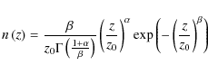$\begin{displaymath}n\left(z\right)=\frac{\beta}{z_0\Gamma\left(\frac{1+\alpha}{\... ...^{\alpha}\exp\left(-\left(\frac{z}{z_0}\right)^{\beta}\right) \end{displaymath}$

(3)

and we fit over the range 0.0 < z < 1.5 for the wide redshift distribution and over the range 0.0 < z < 2.5 for the deep one. Figure 16 shows the redshift distribution derived for the fields W1, W3, W4 and D1, D2, D3, D4 grouped in a wide and deep redshift distributions, respectively. Error bars show the uncertainty for the full deep field, computed from the field-to-field variance between D1, D2, D3 and D4 and multiplied by a factor $1/\sqrt{4}$ , since all 4 deep fields are independent. In the wide field, the field-to-field variance were computed for several subareas and extrapolated to the size of the wide fields and finally divided by $\sqrt 3$ , as the three wide fields are also independent. As expected, the cosmic variance is lower in the wide field which covers $35 \deg^2$ .

$\begin{figure} \par\includegraphics[width=8cm]{1413fig13a.ps} \includegraphics[width=8cm]{1413fig13b.ps} \end{figure}$	Figure 13: Photometric redshift errors as function of magnitude and redshift for both the wide (W1) and the deep fields ( upper panel). Lower panel: a zoom of the redshift range 0.2 < z <1.5.
Open with DEXTER

$\begin{figure} \par\includegraphics[width=8.4cm,clip]{1413fig14.ps} \end{figure}$	Figure 14: Estimated photometric redshift error for the wide (W1) and deep (D1) fields as function of redshift. Errors are binned in redshift with an interval = 0.04. Only a few objects have z>2 in the wide field so errors are less reliable in this range.
Open with DEXTER

$\begin{figure} \par\includegraphics[width=8.4cm,clip]{1413fig15.ps} \end{figure}$	Figure 15: Relative field-to-field variance of subareas in W1 as function of the area (overplotted is the Poisson error). Results are extrapolated to derive an estimate of the total field-to-field variance in the wide field. Uncertainties on the field-to-field variance were derived from the data using a Jackknife estimator.
Open with DEXTER

$\begin{figure} \par\includegraphics[width=8cm]{1413fig16a.ps} \includegraphics[width=8cm]{1413fig16b.ps} \end{figure}$	Figure 16: Redshift distribution in the deep ( top) and wide ( bottom) fields. Error bars comprise the photometric redshift error and the field-to-field variance (cosmic variance and Poisson error).
Open with DEXTER

We estimated the mean redshift of the deep and wide fields for several limiting magnitude. Table 6 shows the mean and median redshift computed directly from the data for several limiting magnitudes. As expected, the mean and median redshifts increase as the limiting magnitude of the sample increases.

The top panel of Fig. 17 compares the wide and deep redshift distributions and their fit for a same magnitude selection at $17.5 < i'_{\rm AB} < 22.5$ . The redshift distributions of the deep and wide fields agree well when the same magnitude limit is adopted.

$\begin{figure} \par\includegraphics[width=8cm]{1413fig17a.ps} \includegraphics[width=8cm]{1413fig17b.ps} \end{figure}$	Figure 17: Distribution of the photometric redshifts ( $i'_{\rm AB} < 22.5$ ) computed on the new data release (T0004) for the wide fields, plotted separately on the lower panel and plotted combined on the upper panel.
Open with DEXTER

Table 6: Mean and median redshifts in the deep and wide fields, for several limiting magnitudes. Both values are computed directly from the data.

Conclusions

We computed photometric redshifts for the release T0004 of the deep and wide CFHT Legacy Survey produced by T ERAPIX. In this work, only T0004 fields observed in all filters (u^*, g', r', i', and z') have been used. Our photometric catalogues cover four independent deep fields of $1\deg^2$ each (D1 to D4) and $35 \deg^2$ distributed over three independent wide fields (W1, W3 and W4).

We define ``reliable'' photometric redshifts as redshifts derived for sources classified as galaxies according to a joint size-colour star-galaxy classification criterion, located in unmasked regions with five-band photometric data and with $\chi^2_{\rm gal} < 1000$ . These objects have a magnitude in the range $17.5 < i'_{\rm AB} < 22.5$ and $17.5 < i'_{\rm AB} < 24$ for the wide and deep samples, respectively. In total, the photometric redshift catalogues contain 244 701 reliable redshifts in the deep field within the magnitude range $17.5 < i'_{\rm AB} < 24$ and 592,891 reliable redshifts in the wide fields within the range $17.5 < i'_{\rm AB} < 22.5$ .

Our photometric redshift method is based on a SED template fitting procedure using the code ``Le Phare''. Following Ilbert et al. (2006) spectroscopic redshifts were used to optimise our SED templates and to correct the systematic offsets between the observations and SEDs. A Bayesian prior is used to break the colour-redshift degeneracies.

A total of 16 983 spectroscopic redshifts from the VVDS deep, VVDS wide, DEEP2 and zCOSMOS spectroscopic surveys provide a spectroscopic coverage for each field (except D4). The large quantity of spectroscopic data enabled an independent systematic offset correction for each field. A mean correction was applied to D4. These offsets vary only by a small amount between the fields, on the order of 0.01 mag, demonstrating the excellent field-to-field stability of the CFHTLS photometry.

We estimated the accuracy of our photometric redshifts by comparing them to spectroscopic catalogues. The deep field photometric redshifts were compared to the VVDS deep and DEEP2 spectroscopic samples limited at $17.5 < i'_{\rm AB} < 24$ , and to the zCOSMOS sample, limited to $i'_{\rm AB} < 22.5$ . We found a stable dispersion of 0.028-0.030 and an outlier rate of about 3-4%. For the wide fields, the dispersion is 0.037-0.039 and the outlier rate is about 3-4% in the range $17.5 < i'_{\rm AB} < 22.5$ (comparing with VVDS deep, VVDS wide and DEEP2). The systematic bias between the input spectroscopic samples and the photometric redshifts derived with Le Phare stays less than 1% over $17.5 < i'_{\rm AB} < 22.5$ for the wide fields and no significant bias is found in the deep fields. We noticed that the dispersion is constant or slightly increasing for S/N > 40, with a more significant increase at lower S/N values. The outlier rate increases dramatically in the wide beyond $i'_{\rm AB}=23$ (5% and 10% at $i'_{\rm AB}<23$ and $i'_{\rm AB} < 24$ ). Our results are comparable to similar analyses conducted in the same CFHTLS wide fields by Erben et al. (2009) and Brimioulle et al. (2008).

Each CFHTLS wide field is composed of several $1\deg^2$ tiles. Unfortunately, the spectroscopic coverage is not sufficient to perform a calibration of the systematic offsets for each tile. We investigated the effect of tile-to-tile photometric offsets on the accuracy of our photometric redshifts. Taking an uncertainty of 0.03 mag for the photometric calibration in each band, we found that the photometric redshifts can be degraded up to 14% in the wide and 21% in the deep. Future wide-field spectroscopic surveys such as VIPERS will help to reduce this effect.

Some wide fields contain as much as 60% of stars at $i'_{\rm AB} < 22.5$ . A reliable galaxy/star separation is important to scientifically exploit these catalogues. We combined both the size and multi-colour data to perform a robust star/galaxy separation. The star selection is purely based on size criteria for the brightest sources ( $i'_{\rm AB} < 21$ ). Since some galaxies are unresolved at fainter magnitudes, we added multi-colour information to avoid rejecting galaxies. Using the spectroscopic data to assess the quality of our classification, we found that our criteria reduces the stellar contamination from 60% (in W4, the field with the highest stellar density) to 8%, while keeping a galaxy sample more than 98% complete. Star contamination is as low as 1-2% in some other fields, like W1 or D1.

Finally, we used the spectroscopic redshifts to evaluate the 68% error estimate computed by ``Le Phare'' for the photometric redshifts. The error distribution, found to be very well approximated by a Gaussian, was in excellent agreement with the real photometric redshift dispersion. Confident with the 68% error estimate for each photometric redshift, we determined the accuracy of our photometric redshifts over a larger magnitude and redshift. Our photometric redshifts are most accurate in the range 0.2 < z < 1.5.

The redshift distributions for the deep and wide fields have been modelled using empirical formula of Van Waerbeke et al. (2001). The distributions and the $z_{\rm median}$ and mean $\langle z\rangle$ derivedfrom the deep and wide samples are consistent with I06, Fu et al. (2008) as well as the recent CFHTLS-wide studies of Erben et al. (2009) and Brimioulle et al. (2008).

The photometric redshifts calculated here will be an essential tool in realising the full potential of the CFHTLS survey. In particular, cosmological parameter estimation, galaxy-galaxy lensing, galaxy biasing studies and investigation of the halo occupation function for galaxies will greatly benefit from this homogeneous and well-calibrated set of photometric redshifts. Additionally, upcoming large spectroscopic surveys like VIPERS will benefit from the increased observing efficiency that pre-selection using photometric redshifts can offer.

Our CFHTLS T0004 deep and wide photometric redshifts are made available to the community through the T ERAPIX and CENCOS databases.

Acknowledgements

We acknowledge the CFHT, T ERAPIX and CADC staff and also the CFHTLS Steering Group for their assistance and considerable work in producing the CFHTLS data. We also acknowledge the VVDS consortium for providing the spectroscopic redshift catalogues. This work has made use of the VizieR catalogue access tool, CDS, Strasbourg. We thank S. Colombi, T. Erben, H. Hildebrandt, B. Ménard, S. Seitz and L. van Waerbeke for useful discussions and advice. MK is supported by the CNRS ANR ``ECOSSTAT'', contract number ANR-BLAN-0283-04. This research has also been supported by the CNRS-ANR grant ``DESIR'' contract number ANR-07-BLAN-0228. We acknowledge the CNRS-Institut National des Sciences de l'Univers (INSU) and the French Programme National de Cosmologie (PNC) for their support for the CFHTLS.

References

Arnouts, S., Cristiani, S., Moscardini, L., et al. 1999, MNRAS, 310, 540 [NASA ADS] [CrossRef]
Arnouts, S., Moscardini, L., Vanzella, E., et al. 2002, MNRAS, 329, 355 [NASA ADS] [CrossRef]
Ball, N. M., Brunner, R. J., Myers, A. D., et al. 2008, ApJ, 683, 12 [NASA ADS] [CrossRef] (In the text)
Benítez, N. 2000, ApJ, 536, 571 [NASA ADS] [CrossRef] (In the text)
Benjamin, J., Heymans, C., Semboloni, E., et al. 2007, MNRAS, 381, 702 [NASA ADS] [CrossRef]
Bergé, J., Pacaud, F., Réfrégier, A., et al. 2008, MNRAS, 385, 695 [NASA ADS] [CrossRef]
Bertin, E. 2006, in Astronomical Data Analysis Software and Systems XV, ed. C. Gabriel, C. Arviset, D. Ponz, & S. Enrique, ASP Conf. Ser., 351, 112 (In the text)
Bertin, E., & Arnouts, S. 1996, A&AS, 117, 393 [NASA ADS] [CrossRef] [EDP Sciences] (In the text)
Bertin, E., Mellier, Y., Radovich, M., et al. 2002, in Astronomical Data Analysis Software and Systems XI, ed. D. A. Bohlender, D. Durand, & T. H. Handley, ASP Conf. Ser., 281, 228 (In the text)
Boulade, O., Charlot, X., Abbon, P., et al. 2000, SPIE Conf. Ser. 4008, ed. M. Iye, & A. F. Moorwood, 657 (In the text)
Brimioulle, F., Lerchster, M., Seitz, S., Bender, R., & Snigula, J. 2008 [arXiv:0811.3211] (In the text)
Brodwin, M., Brown, M. J. I., Ashby, M. L. N., et al. 2006, ApJ, 651, 791 [NASA ADS] [CrossRef] (In the text)
Bruzual, G., & Charlot, S. 2003, MNRAS, 344, 1000 [NASA ADS] [CrossRef] (In the text)
Calzetti, D., Armus, L., Bohlin, R. C., et al. 2000, ApJ, 533, 682 [NASA ADS] [CrossRef] (In the text)
Coleman, G. D., Wu, C.-C., & Weedman, D. W. 1980, ApJS, 43, 393 [NASA ADS] [CrossRef] (In the text)
Davis, M., Faber, S. M., Newman, J., et al. 2003, in Discoveries and Research Prospects from 6- to 10-Meter-Class Telescopes II, ed. P. Guhathakurta, Proc. SPIE, 4834, 161
Davis, M., Guhathakurta, P., Konidaris, N. P., et al. 2007, ApJ, 660, L1 [NASA ADS] [CrossRef]
Erben, T., Hildebrandt, H., Lerchster, M., et al. 2009, A&A, 493, 1197 [NASA ADS] [CrossRef] [EDP Sciences] (In the text)
Fahlman, G., Kaiser, N., Squires, G., & Woods, D. 1994, ApJ, 437, 56 [NASA ADS] [CrossRef] (In the text)
Feldmann, R., Carollo, C. M., Porciani, C., et al. 2006, MNRAS, 372, 565 [NASA ADS] [CrossRef] (In the text)
Fu, L., Semboloni, E., Hoekstra, H., et al. 2008, A&A, 479, 9 [NASA ADS] [CrossRef] [EDP Sciences]
Garilli, B., Le Fèvre, O., Guzzo, L., et al. 2008, A&A, 486, 683 [NASA ADS] [CrossRef] [EDP Sciences] (In the text)
Hildebrandt, H., Wolf, C., & Benítez, N. 2008, A&A, 480, 703 [NASA ADS] [CrossRef] [EDP Sciences] (In the text)
Ilbert, O., Tresse, L., Zucca, E., et al. 2005, A&A, 439, 863 [NASA ADS] [CrossRef] [EDP Sciences] (In the text)
Ilbert, O., Arnouts, S., McCracken, H. J., et al. 2006, A&A, 457, 841 [NASA ADS] [CrossRef] [EDP Sciences] (In the text)
Ilbert, O., Capak, P., Salvato, M., et al. 2009, ApJ, 690, 1236 [NASA ADS] [CrossRef]
Kilbinger, M., Benabed, K., Guy, J., et al. 2009, A&A, 497, 677 [NASA ADS] [CrossRef] [EDP Sciences]
Kinney, A. L., Calzetti, D., Bohlin, R. C., et al. 1996, ApJ, 467, 38 [NASA ADS] [CrossRef] (In the text)
Le Fèvre, O., Guzzo, L., Meneux, B., et al. 2005a, A&A, 439, 877 [NASA ADS] [CrossRef] [EDP Sciences] (In the text)
Le Fèvre, O., Vettolani, G., Garilli, B., et al. 2005b, A&A, 439, 845 [NASA ADS] [CrossRef] [EDP Sciences] (In the text)
Lilly, S. J., Le Fèvre, O., Renzini, A., et al. 2007, ApJS, 172, 70 [NASA ADS] [CrossRef] (In the text)
Magnier, E. A., & Cuillandre, J.-C. 2004, PASP, 116, 449 [NASA ADS] [CrossRef] (In the text)
Margoniner, V. E., & Wittman, D. M. 2008, ApJ, 679, 31 [NASA ADS] [CrossRef] (In the text)
McCracken, H. J., Ilbert, O., Mellier, Y., et al. 2008, A&A, 479, 321 [NASA ADS] [CrossRef] [EDP Sciences]
Mobasher, B., Capak, P., Scoville, N. Z., et al. 2007, ApJS, 172, 117 [NASA ADS] [CrossRef]
Parker, L. C., Hoekstra, H., Hudson, M. J., van Waerbeke, L., & Mellier, Y. 2007, ApJ, 669, 21 [NASA ADS] [CrossRef]
Pickles, A. J. 1998, PASP, 110, 863 [NASA ADS] [CrossRef] (In the text)
Prevot, M. L., Lequeux, J., Prevot, L., Maurice, E., & Rocca-Volmerange, B. 1984, A&A, 132, 389 [NASA ADS] (In the text)
Rowan-Robinson, M., Babbedge, T., Oliver, S., et al. 2008, MNRAS, 386, 697 [NASA ADS] [CrossRef] (In the text)
Schlegel, D. J., Finkbeiner, D. P., & Davis, M. 1998, ApJ, 500, 525 [CrossRef] (In the text)
Schultheis, M., Robin, A. C., Reylé, C., et al. 2006, A&A, 447, 185 [NASA ADS] [CrossRef] [EDP Sciences] (In the text)
Szalay, A. S., Connolly, A. J., & Szokoly, G. P. 1999, AJ, 117, 68 [NASA ADS] [CrossRef] (In the text)
Tereno, I., Schimd, C., Uzan, J.-P., et al. 2009, A&A, 500, 657 [NASA ADS] [CrossRef] [EDP Sciences]
Van Waerbeke, L., Mellier, Y., Radovich, M., et al. 2001, A&A, 374, 757 [NASA ADS] [CrossRef] [EDP Sciences] (In the text)
Wolf, C., Meisenheimer, K., Rix, H.-W., et al. 2003, A&A, 401, 73 [NASA ADS] [CrossRef] [EDP Sciences] (In the text)

Footnotes

... fields: Based on observations obtained with MegaPrime/MegaCam, a joint project of CFHT and CEA/DAPNIA, at the Canada-France-Hawaii Telescope (CFHT) which is operated by the National Research Council (NRC) of Canada, the Institut National des Sciences de l'Univers of the Centre National de la Recherche Scientifique (CNRS) of France, and the University of Hawaii. This work is based in part on data products produced at T ERAPIX and the Canadian Astronomy Data Centre as part of the Canada-France-Hawaii Telescope Legacy Survey, a collaborative project of NRC and CNRS.
... pages: http://terapix.iap.fr/cplt/oldSite/Descart/summarycfhtlswide.html
... pages: http://terapix.iap.fr/rubrique.php?id_rubrique=241
... document: http://terapix.iap.fr/cplt/oldSite/Descart/NewterapixdocT0002.pdf
... SCAMP: http://terapix.iap.fr/soft/scamp
... SWarp: http://terapix.iap.fr/soft/swarp
... page: http://terapix.iap.fr/cplt/oldSite/Descart/summarycfhtlswide.html
... (SDSS): http://www.sdss.org/data
... (VIMOS: http://www.eso.org/sci/facilities/paranal/instruments/vimos/overview.html
... DEIMOS: http://loen.ucolick.org//Deimos/deimos.html
... Phare: http://www.oamp.fr/people/arnouts/LE_PHARE.html
... ERAPIX: http://terapix.iap.fr
... CENCOS: http://cencos.oamp.fr/CFHTLS

All Tables

Table 1: Summary of the data used in this study and in I06.

Table 2: Systematic offsets of $i'_{\rm AB} < 22.5$ limited samples for the deep and wide fields.

Table 3: Photometric redshift accuracy in the W1 and D1 fields for a range of limiting magnitudes.

Table 4: Star/galaxy selection results, the table shows the galaxy incompleteness (Inc.) and the star contamination (Cont.) for the W1 field, with a large PSF size and the highly star crowded field, W4. ``Stars'' represent the intrinsic proportion of stars in the field.

Table 5: Median photometric redshift bias in magnitude slices in the field W1.

Table 6: Mean and median redshifts in the deep and wide fields, for several limiting magnitudes. Both values are computed directly from the data.

All Figures

$\begin{figure} \par\begin{tabular}{c@{}c@{}c@{}} \includegraphics[width=8.5cm]{... ... & \includegraphics[width=8.5cm]{1413fig1d.ps}\\ \end{tabular} \end{figure}$	Figure 1: Sky coverage of the CFHTLS deep fields (D1, D2, D3, D4) and wide fields (W1, W3 and W4) overlapped with spectroscopic surveys: VVDS F02, F22, zCOSMOS and DEEP2.
Open with DEXTER
In the text

$\begin{figure} \par\includegraphics[width=15.5cm,clip]{1413fig2.ps} \end{figure}$	Figure 2: Details of the data processing performed by T ERAPIX.
Open with DEXTER
In the text

$\begin{figure} \par\begin{tabular}{c@{}c@{}c@{}} \includegraphics[width=6cm,cli... ... \includegraphics[width=6cm,clip]{1413fig3f.ps}\\ \end{tabular} \end{figure}$	Figure 3: Photometric redshift accuracy in the deep survey. We compare photometric redshifts with spectro-z's for D1 with VVDS deep ( left), for D2 with zCOSMOS ( middle) and for D3 against DEEP2 ( right). The brighter zCOSMOS survey is limited to $i'_{\rm AB}=22.5$ . In each panel we show the dispersion, $\sigma _{\Delta z/(1+z_{\rm s})} = 1.48 \times median(\vert\Delta z\vert/(1+z_{\rm s}))$ , and the outlier rate, $\eta$ , the proportion of objects with $\vert\Delta z\vert \ge 0.15\times (1+z_{\rm s})$ . In the top panel, triangles represent objects for which we found a second solution in the PDF. In the bottom panel, the object density in the photometric/spectroscopic redshift plane is plotted.
Open with DEXTER
In the text

$\begin{figure} \par\includegraphics[width=8cm,clip]{1413fig4.ps} \end{figure}$	Figure 4: Median signal-to-noise ratio with respect to the limiting magnitude in the wide (W1) and the deep (D1) field. The S/N is $1.0857/\Delta m$ , taken in the i' band. The dashed line represents the median S/N=33, corresponding to the value of the wide sample cut at $i'_{\rm AB} < 22.5$ .
Open with DEXTER
In the text

$\begin{figure} \par\begin{tabular}{c@{}c@{}c@{}} \includegraphics[width=6cm]{14... ...} & \includegraphics[width=6cm]{1413fig5f.ps}\\ \end{tabular} \end{figure}$	Figure 5: Photometric redshift accuracy in the wide survey at $i'_{\rm AB} < 22.5$ . We compare photometric redshifts with spectroscopic ones for the W1 field with the VVDS deep ( left), for W3 with DEEP2 ( middle) and for W4 with VVDS wide ( right). In each panel we show the dispersion, $\sigma _{\Delta z/(1+z_{\rm s})} = 1.48 \times {\rm median}(\vert\Delta z\vert/(1+z_{\rm s}))$ , and the outlier rate, $\eta$ , the proportion of objects with $\vert\Delta z\vert \ge 0.15\times (1+z_{\rm s})$ . In the top panel, triangles represent objects for which we found a second solution in the PDF. Bottom: density of objects in the photometric/spectroscopic redshift plane is plotted.
Open with DEXTER
In the text

$\begin{figure} \includegraphics[width=9cm,clip]{1413fig6a.ps}\\ \includegraphics[width=9cm,clip]{1413fig6b.ps} \end{figure}$	Figure 6: Reduction of the photometric redshift accuracy if the systematic offsets are derived from a given tile and applied to another tile. The results show the variation of the outlier rate ( left panels) and photometric redshift accuracy ( right panels) if the photometry varies of the order of 0.03 mag. Top panels: D1 deep field at $i'_{\rm AB} < 24$ (compared with $\sigma _{\Delta z/(1+z_{\rm s})}=0.028$ and $\eta =3.57\%$ , represented by the red dashed lines, with no variation added in the photometry). Lower panels: W1 wide field at $i'_{\rm AB} < 22.5$ (compared with $\sigma _{\Delta z/(1+z_{\rm s})}=0.037$ and $\eta =2.81\%$ , represented by the red dashed lines, with no photometric perturbation applied).
Open with DEXTER
In the text

$\begin{figure} \includegraphics[width=8cm]{1413fig7.ps} \end{figure}$	Figure 7: Photometric redshifts for the wide field (W1, y-axis) compared with photometric redshifts for the deep field (D1, x-axis). The sample is selected at $17.5 < i'_{\rm AB} < 22.5$ . We fit in the range [0.2, 0.7] to make a better estimate of remaining systematic differences.
Open with DEXTER
In the text

$\begin{figure} \par\begin{tabular}{c@{}c@{}} \includegraphics[width=8cm]{1413fi... ...s} & \includegraphics[width=8cm]{1413fig8b.ps}\\ \end{tabular} \end{figure}$	Figure 8: Star/galaxy separation in one tile of the W1 field, 022539-041200 ( left panel), and one from the W4 field, 221706+002300 ( right panel). Top: $r_{\rm h}$ distribution and the corresponding Gaussian fitting. The red line is the $\mu _{r_{\rm h}}+3\sigma _{r_{\rm h}}$ cut. Bottom: $i'_{\rm AB}$ vs. $r_{\rm h}$ in pixels. Squares and asterisks are VVDS deep and VVDS wide spectroscopically identified galaxies and stars, respectively.
Open with DEXTER
In the text

$\begin{figure} \includegraphics[width=8cm]{1413fig9.ps} \end{figure}$	Figure 9: $\chi ^2$ distributions for ``true'' stars and ``true'' galaxies (according to the VVDS wide spectroscopy) in the field W4. Top: all objects. Middle: objects larger with $r_{\rm h} > r_{\rm hlimit}$ . Bottom: objects with $r_{\rm h} < r_{\rm hlimit}$ .
Open with DEXTER
In the text

$\begin{figure} \par\begin{tabular}{c@{}c@{}} \includegraphics[width=8cm]{1413fi... ... \includegraphics[width=8cm]{1413fig10b.ps}\\ \end{tabular} \par\end{figure}$	Figure 10: Histogram of $\Delta z$ for the wide (W1, W3 and W4, left) and the deep (D1, D3, right) fields. A Gaussian function with a mean of 0 and a dispersion corresponding to the photometric redshift dispersion is superimposed.
Open with DEXTER
In the text

$\begin{figure} \par\begin{tabular}{c@{}c@{}} \includegraphics[width=8cm]{1413fi... ...s} & \includegraphics[width=8cm]{1413fig11b.ps}\\ \end{tabular} \end{figure}$	Figure 11: Cumulative errors for the wide (W1, W3 and W4) and the deep (D1, D3) fields. As expected for a Gaussian error distribution, the photometric redshifts fall within $z_S\pm 1\sigma _{z_{\rm p}}$ 68% of the time where $1\sigma _{z_{\rm p}}$ is the estimated error.
Open with DEXTER
In the text

$\begin{figure} \par\includegraphics[width=8cm]{1413fig12.ps} \end{figure}$	Figure 12: Photometric redshifts errors as function of magnitude and redshift for the deep fields for this study (solid line) and for I06 (dashed line).
Open with DEXTER
In the text

$\begin{figure} \par\includegraphics[width=8cm]{1413fig13a.ps} \includegraphics[width=8cm]{1413fig13b.ps} \end{figure}$	Figure 13: Photometric redshift errors as function of magnitude and redshift for both the wide (W1) and the deep fields ( upper panel). Lower panel: a zoom of the redshift range 0.2 < z <1.5.
Open with DEXTER
In the text

$\begin{figure} \par\includegraphics[width=8.4cm,clip]{1413fig14.ps} \end{figure}$	Figure 14: Estimated photometric redshift error for the wide (W1) and deep (D1) fields as function of redshift. Errors are binned in redshift with an interval = 0.04. Only a few objects have z>2 in the wide field so errors are less reliable in this range.
Open with DEXTER
In the text

$\begin{figure} \par\includegraphics[width=8.4cm,clip]{1413fig15.ps} \end{figure}$	Figure 15: Relative field-to-field variance of subareas in W1 as function of the area (overplotted is the Poisson error). Results are extrapolated to derive an estimate of the total field-to-field variance in the wide field. Uncertainties on the field-to-field variance were derived from the data using a Jackknife estimator.
Open with DEXTER
In the text

$\begin{figure} \par\includegraphics[width=8cm]{1413fig16a.ps} \includegraphics[width=8cm]{1413fig16b.ps} \end{figure}$	Figure 16: Redshift distribution in the deep ( top) and wide ( bottom) fields. Error bars comprise the photometric redshift error and the field-to-field variance (cosmic variance and Poisson error).
Open with DEXTER
In the text

$\begin{figure} \par\includegraphics[width=8cm]{1413fig17a.ps} \includegraphics[width=8cm]{1413fig17b.ps} \end{figure}$	Figure 17: Distribution of the photometric redshifts ( $i'_{\rm AB} < 22.5$ ) computed on the new data release (T0004) for the wide fields, plotted separately on the lower panel and plotted combined on the upper panel.
Open with DEXTER
In the text

Current usage metrics show cumulative count of Article Views (full-text article views including HTML views, PDF and ePub downloads, according to the available data) and Abstracts Views on Vision4Press platform.

Data correspond to usage on the plateform after 2015. The current usage metrics is available 48-96 hours after online publication and is updated daily on week days.

Initial download of the metrics may take a while.