Modeling mm- to X-ray flare emission from Sagittarius A*

A. Eckart; F. K. Baganoff; M. R. Morris; D. Kunneriath; M. Zamaninasab; G. Witzel; R. Schödel; M. García-Marín; L. Meyer; G. C. Bower; D. Marrone; M. W. Bautz; W. N. Brandt; G. P. Garmire; G. R. Ricker; C. Straubmeier; D. A. Roberts; K. Muzic; J. Mauerhan; A. Zensus

doi:10.1051/0004-6361/200811354

Free Access

Issue		A&A Volume 500, Number 3, June IV 2009


Page(s)		935 - 946
Section		Astrophysical processes
DOI		https://doi.org/10.1051/0004-6361/200811354
Published online		29 April 2009

Modeling mm- to X-ray flare emission from Sagittarius A*

A. Eckart^1,2 - F. K. Baganoff³ - M. R. Morris⁴ - D. Kunneriath^1,2 - M. Zamaninasab^1,2 - G. Witzel¹ - R. Schödel⁵ - M. García-Marín¹ - L. Meyer⁴ - G. C. Bower ⁶ - D. Marrone ⁷ - M. W. Bautz³ - W. N. Brandt⁸ - G. P. Garmire⁸ - G. R. Ricker³ - C. Straubmeier¹ - D. A. Roberts ⁹ - K. Muzic^1,2 - J. Mauerhan⁴ - A. Zensus^2,1

1 - I.Physikalisches Institut, Universität zu Köln, Zülpicher Str.77, 50937 Köln, Germany
2 - Max-Planck-Institut für Radioastronomie, Auf dem Hügel 69, 53121 Bonn, Germany
3 - Center for Space Research, Massachusetts Institute of Technology, Cambridge, MA 02139-4307, USA
4 - Department of Physics and Astronomy, University of California Los Angeles, Los Angeles, CA 90095-1562, USA
5 - Instituto de Astrofísica de Andalucía, CSIC, Camino Bajo de Huétor 50, 18008 Granada, Spain
6 - Department of Astronomy and Radio Astronomy Laboratory, University of California at Berkeley, Campbell Hall, Berkeley, CA 94720, USA
7 - Harvard-Smithsonian Center for Astrophysics, Cambridge MA 02138, USA
8 - Department of Astronomy and Astrophysics, Pennsylvania State University, University Park, PA 16802-6305, USA
9 - Department of Physics and Astronomy, Northwestern University, Evanston, IL 60208, USA

Received 16 November 2008 / Accepted 17 March 2009

Abstract
Context. We report on new modeling results based on the mm- to X-ray emission of the SgrA* counterpart associated with the massive $\sim$ $4\times10^6$ $M_{\odot}$ black hole at the Galactic Center.
Aims. We investigate the physical processes responsible for the variable emission from SgrA*.
Methods. Our modeling is based on simultaneous observations carried out on 07 July, 2004, using the NACO adaptive optics (AO) instrument at the European Southern Observatory's Very Large Telescope and the ACIS-I instrument aboard the Chandra X-ray Observatory as well as the Submillimeter Array SMA on Mauna Kea, Hawaii, and the Very Large Array in New Mexico.
Results. The observations revealed several flare events in all wavelength domains. Here we show that the flare emission can be described with a combination of a synchrotron self-Compton (SSC) model followed by an adiabatic expansion of the source components. The SSC emission at NIR and X-ray wavelengths involves up-scattered sub-millimeter photons from a compact source component. At the start of the flare, spectra of these components peak at frequencies between several 100 GHz and 2 THz. The adiabatic expansion then accounts for the variable emission observed at sub-mm/mm wavelengths. The derived physical quantities that describe the flare emission give a blob expansion speed of $v_{\rm exp} \sim 0.005~c$ , magnetic field of B around 60 G or less and spectral indices of $\alpha=0.8$ to 1.4, corresponding to a particle spectral index $p\sim2.6$ to 3.8.
Conclusions. A combined SSC and adiabatic expansion model can fully account for the observed flare flux densities and delay times covering the spectral range from the X-ray to the mm-radio domain. The derived model parameters suggest that the adiabatic expansion takes place in source components that have a bulk motion larger than $v_{\rm exp}$ or the expanding material contributes to a corona or disk, confined to the immediate surroundings of SgrA*.

Key words: black hole physics - X-rays: general - infrared: general - accretion, accretion disks - Galaxy: center - Galaxy: nucleus

1 Introduction

Stellar motion and variable emission allow us to associate Sagittarius A* (SgrA*) at the center of the Milky Way with a super-massive black hole (Eckart & Genzel 1996; Genzel et al. 1997, 2000; Ghez et al. 1998, 2000, 2003, 2005; Eckart et al. 2002; Schödel et al. 2002, 2003; Eisenhauer 2003, 2005).

Recent radio, and near-infrared through X-ray observations have detected flaring and polarized emission and give detailed insight into the physical emission mechanisms at work in SgrA* (e.g. Baganoff et al. 2001, 2002, 2003; Eckart et al. 2003, 2004, 2006a,b, 2008a,b; Porquet et al. 2003, 2008; Goldwurm et al. 2003; Genzel et al. 2003; Ghez et al. 2004a; Eisenhauer et al. 2005; Hornstein et al. 2007; Yusef-Zadeh et al. 2006a,b, 2007, 2008; Marrone et al. 2008).

Variability at radio through sub-millimeter wavelengths has been studied extensively, showing that variations occur on timescales from hours to years (Wright & Backer 1993; Bower et al. 2002, 2003, 2004, 2005a, 2006; Herrnstein et al. 2004; Zhao et al. 2003, 2004; Eckart et al. 2006a; Mauerhan et al. 2005; Yusef-Zadeh et al. 2007, 2008; Miyazaki et al. 2006; Marrone et al. 2008). Several flares have provided evidence for decaying millimeter and sub-millimeter emission following NIR/X-ray flares. Simultaneous multi-wavelength observations indicate the presence of adiabatically expanding source components with a delay between the X-ray and sub-mm flares of about 100 min (Eckart et al. 2006a; Yusef-Zadeh et al. 2008; Marrone et al. 2008). The adiabatic expansion is also supported by the expected swing in polarization as indicated by the measurements of Yusef-Zadeh et al. (2008). From modeling the mm-radio flares at individual frequencies Yusef-Zadeh et al. (2007, 2008) invoke expansion velocities in the range from $v_{\rm exp}=0.003-0.1~c$ . This is also supported by the results of recent NIR/sub-mm observations in May 2008 using NACO at the VLT and the LABOCA bolometer at the Atacama Pathfinder Experiment (APEX), at 0.87 mm wavelength (345 GHz) (Eckart et al. 2008b; García-Marín 2008, in prep.). Here we find an expansion speed of 0.005 c. The speed is well below the asymptotic upper limit of $c/\sqrt{3}$ obtained for a system of relativistically interacting particles (e.g. Bowers 1972) expected in the vicinity of the super-massive black hole (Blandford & McKee 1977). It is also low compared to the expected orbital velocities that may be of the order of 0.5 c close to the last stable orbit around the SMBH. The low expansion velocities suggest that the expanding gas cannot escape from SgrA* or must have a large bulk motion (Yusef-Zadeh et al. 2008; Eckart et al. 2008b).

In order to investigate this question in more detail we revisited the first observations of a flare with simultaneous coverage in the NIR/X-ray and sub-mm/mm wavelength domain observed on July 07, 2004. Eckart et al. (2006a) showed that the observed amplitudes of the flux density variations are generally consistent with adiabatic expansion of a synchrotron self-absorbed source (van der Laan 1966). Here we present a detailed time dependent model of the flare emission from the X-ray to the short cm-wavelength domain.

For optically thin synchrotron emission we refer throughout this paper to photon spectral indices ( $\alpha$ ) using the convention $S_\nu\propto\nu^{-\alpha}$ and to spectral indices (p) of electron power-law distributions using $N(E)\propto E^{-p}$ with $p=\left(1+2\alpha\right)$ . The assumed distance to SgrA* is 8 kpc (Reid 1993), consistent with more recent results (e.g. Ghez et al. 2005; Eisenhauer et al. 2003).

Table 1: NIR/X-ray flare flux densities.

2 Observations and data reduction

In 2004 from July 05 to 08 Sgr A* was observed from the radio millimeter to the X-ray wavelength domain. On July 07 a strong simultaneous NIR/X-ray flare event was observed immediately followed by simultaneous SMA and VLA observations. Putting emphasis particularly on the NIR/X-ray data the details for the entire observing run have been analyzed in Eckart et al. (2006a). For completeness we give in the following a brief summary of the data acquisition and reduction for the X-ray, NIR and sub-mm/mm domain with emphasis on the essentials important for the presented analysis. The observational results are summarized in Table 1. There the peak flux densities of the flares detected in the individual wavelength bands are given. The X-ray flares $\phi$ 2, $\phi$ 3 and $\phi$ 4 have been detected simultaneously in the NIR (Eckart et al. 2006a). Individual AO images for the NIR event II presented by Eckart et al. (2006a) as well as the newly reduced light-curve shown here in Fig. 2 demonstrate that Sgr A* clearly was in an ``on'' state.

$\begin{figure} \par\includegraphics[width=8.5cm,clip]{11354-f1.eps} \end{figure}$

Figure 1:

The X-ray and NIR 2.2 $\mu$ m light curves obtained on July 07, 2004 (Eckart et al. 2006a). Here we plot the data with a UT time axis and separate flux density axes for the NIR ( left) and X-ray ( right) data. In addition to the flare nomenclature introduced in Eckart et al. (2006a) we labeled the section of the X-ray light curve that corresponds to the NIR feature II as $\phi$ 2/3 as it is located between $\phi$ 2 and $\phi$ 3.

Open with DEXTER

2.1 The NACO NIR adaptive optics observations

Near-infrared (NIR) observations of the Galactic Center (GC) were carried out with the NIR camera CONICA and the adaptive optics (AO) module NAOS (briefly ``NACO'') at the ESO VLT unit telescope 4 on Paranal, Chile, during the nights between 05 July and 08 July 2004. In all observations, the infrared wavefront sensor of NAOS was used to lock the AO loop on the NIR bright (K-band magnitude $\sim$ 6.5) supergiant IRS 7, located about 5.6'' north of Sgr A*. All exposures were sky subtracted, flat-fielded, and corrected for dead or bad pixels. In order to enhance the signal-to-noise ratio of the imaging data, we created median images comprising 9 single exposures each. Subsequently, PSFs were extracted from these images with StarFinder (Diolaiti et al. 2000). The images were deconvolved with the Lucy-Richardson (LR) and linear Wiener filter (LIN) algorithms. Beam restoration was carried out with a Gaussian beam of FWHM corresponding to the final resolution at 2.2 $\mu$ m of 60 milli-arcsec. The flux densities of the sources were measured by aperture photometry with circular apertures of 52 mas radius and corrected for extinction, using A_K = 2.8. Calibration of the photometry and astrometry was done with the known fluxes and positions of 9 sources within 1.6'' of Sgr A*.

In Fig. 1 we show the July 07 NIR and X-ray data in comparison. Four NIR flares (I-IV) can be identified. In Fig. 11 of Eckart et al. (2006a) individual AO images correspond to separate points in time and include the flares discussed here. These images demonstrate that even during the weak NIR flare feature II Sgr A* clearly was in an ``on'' state and significantly weaker before and after. For the flare feature II the NIR flux density excess is of the order of 3 mJy.

To re-assess the presence of the flare zone II we re-reduced the NIR data and show the results in Fig. 2. The re-reduction includes the following additional features: 1) we used sub-pixel shifting of the data applying the ``jitter''-routine in ECLIPSE (Devillard 1997); 2) we subtracted a constant background based on a StarFinder analysis; 3) we rejected low quality images based on the number of stars detected by StarFinder; 4) we removed low level common trends ( $\le$ 15%) that became apparent in the reference star data by applying a detrending routine (by Nicolas Marchili, IMPRS, MPIfR). The generation of the trend involves binning and splining of the reference star data and is similar to a procedure described in Villata et al. (2004). The resulting trend then is then removed from the SgrA* NIR light curve as well; 5) for comparison we also plot the FWHM of the nearby reference stars as an indication of the combined instantaneous NIR seeing and the quality of the AO correction.

We find that within the uncertainties the result of the re-reduction is in very good agreement with the original data reduction used in Fig. 1. The improved analysis shows that flare zone II is a reliably feature in the NIR light curve.

2.2 The Chandra X-ray observations

In parallel to the NIR observations, SgrA* was observed with Chandra using the imaging array of the Advanced CCD Imaging Spectrometer (ACIS-I, Weisskopf et al. 2002) for two blocks of $\sim$ 50 ks on 05-07 July 2004 (UT). We reduced and analyzed the data using CIAO v2.3 software with Chandra CALDB v2.22.

$\begin{figure} \par\includegraphics[width=9cm,clip]{11354-f2.eps} \end{figure}$

Figure 2:

Results of the re-reduction of the NIR 2.2 $\mu$ m data from July 07, 2004 In panel a) the flux density scale is given in mJy. The top (green) data points represent the light curve of the nearby flux star S1 used for flux density calibration and the black data points with the blue interpolation line represent the SgrA* light curve. The time axis is given in minutes offset from the start time at 23:19:38 UT on 6 July 2004 and in UT hours at the bottom. In the bottom panel b) we show the FWHM of the PSF in the AO images that reflect the combination of AO correction and input seeing.

Open with DEXTER

We extracted counts within radii of 0.5 $^{\prime\prime}$ , 1.0 $^{\prime\prime}$ , and 1.5 $^{\prime\prime}$ around Sgr A* in the 2-8 keV band. Background counts were extracted from an annulus around Sgr A* with inner and outer radii of 2 $^{\prime\prime}$ and 10 $^{\prime\prime}$ , respectively, excluding regions around discrete sources and bright structures (Baganoff et al. 2003). The mean (total) count rates within the inner radius subdivided into the peak count rates during a flare and the corresponding intermediate quiescent flux values are listed in Table 4 in Eckart et al. (2006a). The background rates have been scaled to the area of the source region. The 1.0 $^{\prime\prime}$ aperture provides the best compromise between maximizing source signal and rejecting background. In Fig. 1 we have labeled the section of the X-ray light curve that corresponds to the NIR feature II as $\phi$ 2/3, as it is located between $\phi$ 2 and $\phi$ 3. For $\phi$ 2/3 the X-ray flux density excess above the quiescent bremsstrahlung component of SgrA* is below 20 nJy.

2.3 The SMA observations

The sub-millimeter observations were made with the Submillimeter Array (SMA) on Mauna Kea, Hawaii (Ho et al. 2004). The observations of SgrA* were made at 340 GHz (890 $\mu$ m wavelength) for three consecutive nights, 05-07 July 2004 (UT), at an angular resolution of $1\hbox{$.\!\!^{\prime\prime}$ }5\times3\hbox{$.\!\!^{\prime\prime}$ }0$ . Nearby quasars were used for phase and gain calibration. On both July 6 and 7 we obtained more than 6 h of simultaneous X-ray/sub-millimeter coverage with 340 GHz zenith opacities from 0.11 to 0.29 for July 5 to 7, respectively. This is reflected in the larger time bins and scatter in the later light curves.

The same 5 antennae with the best gain stability were used to form light curves, resulting in a typical synthesized beam of $1\hbox{$.\!\!^{\prime\prime}$ }5\times3\hbox{$.\!\!^{\prime\prime}$ }0$ . The SgrA* data are phase self-calibrated after the application of the quasar gains to remove short-timescale phase variations, then imaged and cleaned. Finally, the flux density is extracted from a point source fit at the center of the image, with the error taken from the noise in the residual image. The overall flux scale is set by observations of Neptune, with an uncertainty of approximately 25%.

We attribute a flux density value of $\sim$ 2.4 Jy as a constant or only slowly variable part or the light curve that may be due to more extended source components. Since the final data point in the July 07 light curve is significantly below the minimum of $\sim$ 2.4 Jy that is usually obtained on SgrA* at 340 GHz (e.g. Yusef-Zadeh et al. 2008; Marrone et al. 2008) and due to the steep drop in flux density towards the end of the observations at low elevations we did not consider this data point in our models of the light curve.

2.4 The VLA 7 mm observations

The Very Large Array (VLA) observed Sgr A* for $\sim$ 5 h on 6, 7 and 8 July 2004 at 43 GHz (7 mm wavelength). Observations covered roughly the UT time range 04:40 to 09:00, which is a subset of the Chandra observing time on 6 and 7 July. Observations on 7 July immediately followed the VLT NIR observations. The VLA was in D configuration and achieved a resolution of $2.5 \times 0.9$ arcsec at the observing wavelength of 0.7 cm. The absolute amplitude calibration was set by observations of 3C 286. Flux densities were determined for Sgr A* and J1744-312 through fitting of visibilities at (u,v) distances greater than 50 k $\lambda$ in order to remove contamination from extended structure in the Galactic Center.

In Fig. 3 we show the 340 GHz SMA and 43 GHz VLA total intensity light curves from July 07. Here the July 07 VLA light curve was calculated as the difference between the mean flux density data at the same interferometer hour angle obtained on July 06 and 08 (see Fig. 8 in Eckart et al. 2006a). The minimum compact flux density of $\sim$ 1.4 Jy obtained between 7 and 8 h UT has to be added to the resulting excess flux density in order to derive a complete 43 GHz light curve of SgrA* obtained in the VLA D configuration at an angular resolution of $2\hbox{$.\!\!^{\prime\prime}$ }5\times0\hbox{$.\!\!^{\prime\prime}$ }9$ .

3 Radiation mechanisms

Due to the short flare duration the flare emission very likely originates from compact source components. The simultaneous X-ray/NIR flare detections of the SgrA* counterpart implies that the same population of electrons is responsible for both the IR and the X-ray emission (e.g. Eckart et al. 2004). The spectral energy distribution of SgrA* is currently explained by models that invoke radiatively inefficient accretion flow processes (RIAFs: Quataert 2003; Yuan et al. 2002; Yuan et al. 2003, 2004, including advection dominated accretion flows (ADAF): Narayan et al. 1995, convection dominated accretion flows (CDAF): Ball et al. 2001; Quataert & Gruzinov 2000; Narayan et al. 2002; Igumenshchev 2002, advection-dominated inflow-outflow solution (ADIOS): Blandford & Begelman 1999; see also Ballantyne, Özel et al. 2005), jet models (Markoff et al. 2001; see also Markoff 2005), and Bondi-Hoyle models (Melia & Falcke 2001). Also combinations of models such as an accretion flow plus an outflow in the form of a jet are considered (e.g. Yuan et al. 2002).

$\begin{figure} \par\includegraphics[width=8cm,clip]{11354-f3.eps} \end{figure}$

Figure 3:

340 GHz SMA and 43 GHz VLA total intensity light curves from July 07. The individual data points are connected by straight lines. The July 07 VLA data represent the excess flux density compared to the mean of the July 06 and 08 VLA data. The constant flux density of about 1.4 Jy that has to be added to this excess is indicated by a dashed line. For further details see text and Eckart et al. (2006a).

Open with DEXTER

3.1 Adiabatically expanding source components

To model the sub-mm/mm light curves we assume an expanding uniform blob of relativistic electrons with an energy spectrum $n(E) \propto E^{-p}$ threaded by a magnetic field. As the blob expands, the magnetic field declines with increasing blob radius as R^-2, the energy of relativistic particles as R^-1 and the density of particles as R^-3(van der Laan 1966). The synchrotron optical depth at frequency $\nu$ then scales as

$\begin{displaymath}\tau_\nu = \tau_0 \left(\frac{\nu}{\nu_0}\right)^{-(p+4)/2} \left(\frac{R}{R_0}\right)^{-(2p+3)} \end{displaymath}$

(1)

and the flux density scales as

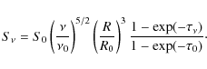
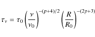
$\begin{displaymath}S_\nu = S_0 \left(\frac{\nu}{\nu_0}\right)^{5/2} \left(\frac{R}{R_0}\right)^3 \frac{1-\exp(-\tau_\nu)}{1-\exp(-\tau_0)}\cdot \end{displaymath}$

(2)

Since the goal is to combine the description of an adiabatically expanding cloud with a synchrotron self-Compton formalism we use the definition of $\tau_0$ as the optical depth corresponding to the frequency at which the flux density is a maximum (van der Laan 1966) rather than the definition of $\tau_0$ as the optical depth at which the flux density for any particular frequency peaks (Yusef-Zadeh et al. 2006b). Therefore $\tau_0$ depends only on p through the condition

$\begin{displaymath}{\rm e}^{\tau_0} - \tau_0(p + 4)/5 - 1 = 0 \end{displaymath}$

(3)

and ranges from 0 to 0.65 as p ranges from 1 to 3. Thus given the particle energy spectral index p and the peak flux S₀ in the light curve at some frequency $\nu_0$ , this model predicts the variation in flux density at any other frequency as a function of the expansion factor (R/R₀).

A model for R(t) is required to convert the dependence on radius to time: we adopt a simple linear expansion at constant expansion speed $v_{\rm exp}$ , so that $R-R_0 = v_{\rm exp}~(t-t_0)$ . Here we assume that the source component is decoupled from energy input and is freely expanding, i.e. neither accelerations nor decelerations of the expansion are dominant (see end of Sect. 4.1.4). A possible magnetic confinement of the spot will be described in the model as a low expansion speed, i.e. it is contained in the model of R(t). For $t \le t_0$ we have made the assumption that the source has an optical depth that equals its frequency dependent initial value $\tau_{\nu}$ at R = R₀. So in the optically thin part of the source spectrum the flux initially increases with the source size at a constant $\tau_{\nu}$ and then decreases due to the decreasing optical depth as a consequence of the expansion. For the $\sim$ $4\times10^6$ $M_{\odot}$ super-massive black hole at the position of Sgr A*, one Schwarzschild radius is $R_{\rm s}=2GM/c^2\sim10^{10}$ m and the velocity of light corresponds to about 100 $R_{\rm s}$ per hour. For t > t₀ the decaying flank of the curve can be shifted towards later times by first increasing the turnover frequency $\nu_0$ or the initial source size R₀, and second, by lowering the spectral index $\alpha_{\rm synch}$ or the peak flux density S₀. Increasing the adiabatic expansion velocity $v_{\rm exp}$ shifts the peak of the light curve to earlier times. Adiabatic expansion will also result in a slower decay rate and a longer flare timescale at lower frequencies. Throughout the paper we give R(t) and R₀ in units of the Schwarzschild radius $R_{\rm s}$ .

3.2 Description and properties of the SSC model

We have employed a simple SSC model to describe the observed radio to X-ray properties of SgrA* using the nomenclature given by Gould (1979) and Marscher (1983). Inverse Compton scattering models provide an explanation for both the compact NIR and X-ray emission by up-scattering sub-mm-wavelength photons into these spectral domains. Such models are considered as a possibility in most of the recent modeling approaches and may provide important insights into some fundamental model requirements. The models do not explain the entire low frequency radio spectrum and the bremsstrahlung X-ray emission that dominates the IQ state. Also high power X-ray fares (e.g. Porquet et al. 2003, 2008) may involve additional emission mechanisms. However, for X-ray flares of up to several 10 times the quiescent emission the SSC models provide a successful description of the compact IQ and flare emission originating from the immediate vicinity of the central black hole. A more detailed explanation is also given by Eckart et al. (2004).

We assume a synchrotron source of angular extent $\theta$ . The source size is of the order of a few Schwarzschild radii $R_{\rm s}=2GM/c^2$ with $R_{\rm s} \sim10^{10}$ m for a $\sim$ $4\times10^6$ $M_{\odot}$ black hole. One $R_{\rm s}$ then corresponds to an angular diameter of $\sim$ 8 $\mu$ as at a distance to the Galactic Center of 8 kpc (Reid 1993; Eisenhauer et al. 2003; Ghez et al. 2005). The emitting source becomes optically thick at a frequency $\nu_{\rm m}$ with a flux density $S_{\rm m}$ , and has an optically thin spectral index $\alpha$ following the law $S_\nu\propto\nu^{-\alpha}$ . This allows us to calculate the magnetic field strength B and the inverse Compton scattered flux density $S_{\rm SSC}$ as a function of the X-ray photon energy $E_{\rm keV}$ . The synchrotron self-Compton spectrum has the same spectral index as the synchrotron spectrum that is up-scattered i.e. $S_{\rm SSC} \propto E_{\rm keV}^{-\alpha}$ , and is valid within the limits $E_{\rm min}$ and $E_{\rm max}$ corresponding to the wavelengths $\lambda_{\rm max}$ and $\lambda_{\rm min}$ (see Marscher et al. 1983, for further details). We find that Lorentz factors $\gamma_{\rm e}$ for the emitting electrons of the order of typically 10³ are required to produce a sufficient SSC flux in the observed X-ray domain. A possible relativistic bulk motion of the emitting source results in a Doppler boosting factor $\delta=\Gamma^{-1}(1-\beta \cos \phi)^{-1}$ . Here $\phi$ is the angle of the velocity vector to the line of sight, $\beta$ the velocity v in units of the speed of light c, and Lorentz factor $\Gamma=(1-\beta^2)^{-1/2}$ for the bulk motion. Relativistic bulk motion is not a necessity to produce sufficient SSC flux density but we have used modest values for $\Gamma=1.2{-}2$ and $\delta$ ranging between 1.3 and 2.0 (i.e. angles $\phi$ between about $10^{\circ}$ and $45^{\circ}$ ) since they will occur in cases of relativistically orbiting gas as well as relativistic outflows - both of which are likely to be relevant to SgrA*.

$\begin{figure} \par\includegraphics[width=8.1cm,clip]{11354-f4.eps} % \par \end{figure}$	Figure 4: A comparison of a 340 GHz light curve calculated with adiabatic expansion velocities that differ by factors of two.
Open with DEXTER

4 Modeling the light curves

Our primary goal was to generate a model that includes the entire data set on the flare event observed on July 7, 2004 from the mm- to the X-ray domain. Models like F1 or F2 (Eckart et al. 2006, their Table 9) or the dynamical, multicomponent model presented by Eckart et al. (2008a) reproduce the NIR/X-ray properties of the observed flare $\phi$ 3/III and $\phi$ 4/IV very well. We have repeated this modeling under the premise of achieving fits with a simultaneous match to the SMA and VLA data.

The six so far reported coordinated SgrA* measurements that include sub-mm data (Eckart et al. 2006b; Yusef-Zadeh et al. 2006b; Marrone et al. 2008; Eckart et al. 2008b) have shown that the observed submillimeter flares follow strong NIR or X-ray events. If the events were unrelated we would expect an equal number of submillimeter flares leading and following the NIR/X-ray events (see detailed discussion in Marrone et al. 2008). We therefore assume that the sub-millimeter flare presented here is related to the observed IR flare events.

$\begin{figure} \par\includegraphics[width=8.5cm,clip]{11354-f5.eps} \end{figure}$	Figure 5: The adiabatic expansion of a single source component with a peak flux density at 1.64 THz of 10 Jy, start time at 0 hours, and constant expansion velocity of 0.08 c. The 1.64 THz, 8 THz and 32 THz light curves have been scaled down by a factor of 5.2.
Open with DEXTER

For the July 7 SMA and VLA data Eckart et al. (2006a) have shown that the observed amplitudes of the flux density variations are generally consistent with adiabatic expansion of a synchrotron self-absorbed source (van der Laan 1966). Following the THz peaked NIR/X-ray flare events III/ $\phi3$ and IV/ $\phi4$ on July 7 (see Fig. 1 and modeling results given by Eckart et al. 2006a) the radio flux density will first rise and later drop as the source evolves.

However, a detailed comparison to theoretical light curves of adiabatically expanding source components shows that a single source component cannot give a satisfactory fit to the sub-mm/mm data. In Fig. 5 we show that when the 340 GHz light curve is decaying, the 43 GHz curve is still rising (straight bold face section in the correponding lines). When the 43 GHz curve is decaying then the decaying 340 GHz light curve is at flux density levels well below the 43 GHz curve (dashed bold face section in the correponding lines). Both scenarios are inconsistent with the observations on July 04. This result is also independent of the expansion velocity. Modeling the 2004 July 07 radio data therefore must involve a minimum of two source components. Quite naturally two components can be associated with the NIR/X-ray flares III/ $\phi$ 3 and IV/ $\phi$ 4.

Our goal is to fit the variable part of the sub-mm/mm light curves (see Sect. 2.3) with a source model that is also able to describe the observed NIR/X-ray properties. We calculated model light curves at 340 GHz and 43 GHz for the model with a smallest (4) and larger (6) number of source components. Smaller numbers of components cannot account for all essential features of the sub-mm/NIT/X-ray light curves. A detailed explanation is given in the following.

$\begin{figure} \par\includegraphics[width=7cm,clip]{11354-f6.eps} \end{figure}$	Figure 6: Decomposition of the 340 GHz and 43 GHz light curve for model B1 (see Table 3) into the contributions of the different source components ( $\alpha$ to $\zeta$ ). The data are shown with the offsets discussed in Sects. 2.3 and 2.4 removed.
Open with DEXTER

$\begin{figure} \par\includegraphics[width=7cm,clip]{11354-f7.eps} \end{figure}$	Figure 7: The observed 43 GHz and 340 GHz light curves shown in comparison to model A1, B1, and C1. The data is shown with the offsets discussed in Sects. 2.3 and 2.4 removed.
Open with DEXTER

In Fig. 6 we show the decomposition of the overall light curves into the contribution of individual source components. In Figs. 7 and 8 we show the model light curves for comparison to the measured 340 GHz and 43 GHz data.

SSC modeling with adiabatically expanding source components: we iterated between the SSC modeling of the NIR/X-ray data and the modeling of the sub-mm/mm data as adiabatically expanding sources using the same component parameters as given in Table 3. The source expansion is also motivated by an indication of a hot spot evolution within a possible accretion disk based on a May 2007 flare event. Eckart et al. (2008a) have described the July 2004 flare using a multi-component disk model allowing for a source size increase of (at least) 30% over about 40 min in order to explain the strong decrease of the X-ray flux density between $\phi$ 3 and $\phi$ 4.

$\begin{figure} \par\includegraphics[width=8.5cm,clip]{11354-f8.eps} \end{figure}$	Figure 8: The observed 43 GHz and 340 GHz light curves shown in comparison to model C2. The data is shown with the offsets discussed in Sects. 2.3 and 2.4 removed.
Open with DEXTER

In Table 3 we summarize the properties of 6 different models that we considered to represent the 2004 July 7 radio, NIR, and X-ray data. For each model the `` $\times$ '' symbols in Cols. 2 and 3 indicate which of the source components have been considered for the models. Correspondingly they are labeled A1, A2, B1, B2, C1 and C2. The offset times $\Delta$ t are given with respect to the peak of the brighter NIR flares $\phi$ 3 (synchronous with the brightest X-ray flare III) at about 7 July, 204, 03:15:00 UT. The 340 GHz flare SMA5 is accounted for by either a double ( $\gamma, \delta$ ) or a single ( $\eta$ ) component in A1, B1, C1 and A2, B2, C2, respectively, using the source labels marked in Cols. 1-3. The decaying 43 GHz flux density component VLA1 is accounted for by simple flux density offsets in models A1 and A2 (see caption of Table 3) or by 2 components ( $\epsilon, \zeta$ ) in models (B1, B2, C1, C2). In Col. 4 the individual adiabatically expanding source components are labeled and identified with the flares detected in the different wavelength regimes using the nomenclature by Eckart et al. (2006a) and here (see Fig. 1). The modeling was done with constant expansion velocities of 0.005 c for models (A, B) and 0.006 c for models (C). In Table 3 the flux density offsets of the VLA and SMA data used for models A1/A2 are 0.26 Jy and 1.9 Jy. Flux density offsets of the VLA and SMA data used for models B1/B2/C1/C2 and are 0.0 Jy and 1.8 Jy, respectively. The $\Delta \chi$ values in comparison to the mm/sub-mm data that we obtained for the various models are: A1: 2.9; A2: 3.1; B1: 1.71; B2: 1.81; C1: 1.70; C2: 1.80. Results of the modeling are discussed in Sect. 4.1.

The predictions from the SSC-modeling and of the optically thin NIR flux density from the sub-mm data are especially sensitive to variations of the model parameters. The uncertainties of the model parameters given in the first row of Table 3 were derived from a comparison of observed and predicted NIR and X-ray model flux densities and from reduced $\chi^2$ values calculated by comparing the SMA and VLA data with the adiabatic expansion models.

A global variation of a single parameter by the value listed in the corresponding column results in an increase of $\Delta \chi = 1$ . Here global variation means: adding for a single model parameter but for all source components the 1 $\sigma$ uncertainty, such that a maximum positive or negative flux density deviation is reached.

Alternatively, a variation by the listed uncertainty for only a single source component results in a variation of the model predicted NIR and X-ray flux density by more than 30%. Judging from the $\Delta \chi$ based on the sub-mm data only the global uncertainties for $S_{\rm max, obs}$ , $\alpha_{\rm synch}$ and R₀ could be doubled.

The minimum number of source components is 5. In the reduced $\chi^2$ fit we used 5 times 4 ( $S_{\rm max}$ , $\alpha_{\rm synch}$ , R₀, $\nu_{\rm max}$ ) plus one common expansion velocity $v_{\rm exp}$ and time offset (leaving the time differences between the components fixed), i.e. 22 degrees of freedom. The model parameters can unfortunately not all be considered as being independent, e.g. the width and peak of a light curve signature depends to a varying extend on all 4 parameters $S_{\rm max}$ , $\alpha_{\rm synch}$ , R₀, and $\nu_{\rm max}$ . Therefore we stayed for all models with the minimum number of source components (5) to estimate the degrees of freedom. Leaving all parameters free ( $\Delta t$ , $v_{\rm exp}$ , $S_{\rm max}$ , $\alpha_{\rm synch}$ , R₀, and $\nu_{\rm max}$ ) would double the number of degrees of freedom and reduce the $\chi^2$ values correspondingly. Since the VLA data consists of 5 to 6 times the number of SMA data points we weighted the squared SMA flux deviations and number of data points by factor of 6. The $\chi^2$ test was then carried out using the sum of the squared flux deviations and data points of the VLA and SMA datasets.

Of course the models have been set up under the constraint of minimizing the number of free parameters (and to maximize the description of significant flare features in the observed light curves). The flux excursions labeled (VLA1, $\phi$ 2/3) could easily be explained by 3 or 4 components rather than 2 ( $\epsilon$ and $\zeta$ ) in the same way as SMA5 can be explained by 2 ( $\gamma$ and $\delta$ ) rather than a single component ( $\eta$ ).

In the following we comment on the detailed modeling of different sections of the light curves.

Modeling of individual portions of the light curves: significant NIR and X-ray flux density is only produced from the initial THz peaked source components $\alpha$ and $\beta$ . Using a linear expansion at constant speed $v_{\rm exp}$ we then calculate light curves in the selected sub-mm/mm bands. For an expansion speed of $\sim$ 0.005 c we find that the radio model component $\beta$ (due to the III/ $\phi3$ NIR/X-ray flare event) can account for a major portion of the decreasing part of the 340 GHz light curve - SMA4 in Fig. 3 - between 06 and 12 UT on July 2004.

Components $\alpha$ and $\beta$ also account for a portion of the final section (after about 6 h UT - VLA1 in Fig. 3) of the decreasing 43 GHz light curve. For models A and B the spectral indices of components $\alpha$ and $\beta$ of $\alpha_{\rm synch}=0.8$ are consistent with the value of $0.6\pm0.2$ found by Hornstein et al. (2007; see discussion in Sect. 4.1.1). While the NIR flux density in models (A, B) is provided by direct synchrotron emission, the flux density in model (C) is produced via the low frequency section of the scattered SSC specrum. In this case the spectral index must be steep ( $\alpha_{\rm synch}=1.2$ ) and is close to the value derived for the overall NIR/X-ray spectral index of $\alpha$ and $\beta$ of $\alpha_{\rm NIR/X{-}ray}=1.2 \pm0.2$ (Eckart et al. 2006a). This is consistent with the fact that the optically thin synchrotron spectral index (sub-mm to NIR) is expected to equal the broad band spectral index of the SSC spectrum.

Components $\alpha$ and $\beta$ cannot fully account for the 43 GHz radio flux density. This is especially true for the the initial section (before 6 h UT) of the decreasing 43 GHz light curve. The remaining flux density of the VLA1 flare event then has to be explained by source components that provide an almost flat light curve between 5 and 9 h UT. Alternatively, source components that can be identified with the the NIR flare component II/ $\phi$ 2/3 (see Fig. 1) are required to deliver this flux density contribution. To model the light curve in this region a minimum of 2 model components ( $\zeta$ and $\epsilon$ ) is needed. The observed flux densities (or limits) and implied time differences require rather steep spectral indices of $\alpha_{\rm synch}=1.3$ for these source components. Especially for models C1 and C2 the predicted peak flux densities for the 340 GHz and 43 GHz bands lie well within the range of observed flux density values (e.g. Marrone et al. 2008; Yusef-Zadeh et al. 2008; Eckart et al. 2006a).

The 340 GHz flare event SMA5 requires at least one ( $\eta$ ) or two model components ( $\gamma$ , $\delta$ ). For two source components a steep spectral index with $\alpha_{\rm synch}=0.9{-}1.4$ results in a weak NIR flare event with an X-ray flux that would have been non-detectable for Chandra in the presence of the quiescent X-ray bremsstrahlung component of SgrA*. For a single component a flat spectral index of $\alpha_{\rm synch}=0.2$ (corresponding to p=0.6) is required. This results in a significant NIR/X-ray flare about $4\pm1$ h after the III/ $\phi3$ flare event. Figure 6 in Eckart et al. (2006a) shows that no X-ray event was detected by Chandra over this period of time. Therefore a flat spectral component $\eta$ can be excluded.

4.1 Discussion of the modeling results

Our modeling shows that the observed mm through X-ray data of the July 7, 2004 flare event can be successfully modeled by a combination of an SSC and an adiabatic expansion model. While our analysis cannot fully support or even prove the model of adiabatic expansion for the flare emission of SgrA* by itself, it is in full agreement with model results that have been obtained by analyzing previous observations (e.g. Eckart et al. 2006a, 2008b; Yusef-Zadeh et al. 2007, 2008; Marrone et al. 2008). The modeling also suggests the presence of two flare phases in the simultaneous NIR/X-ray events. The fact that a single component adiabatic expansion model cannot account for the observed sub-mm/mm light curves, the considerable spread in source parameters (brightness, size, spectal index, sub-mm turnover frequency) as well as the presence of a non rapidly variable (on timescale of more than one or a few days) flux density component indicates low level activity in addition to the presence of repeated individual bright flares. The flare event II/ $\phi$ 2/3 probably is an example of such low level activity.

Our modeling also requires the low adiabatic expansion velocity that describes other flares of SgrA* (Yusef-Zadeh et al. 2007, 2008; Eckart et al. 2008b). Our values of $\sim$ 0.005 c fits well into the range of velocities of $v_{\rm exp}=0.003{-}0.1$ c given by Yusef-Zadeh et al. (2008). It is currently unclear how to interpret the expansion velocity. The velocities are lower than the orbital velocities for flare components introduced from orbiting spot models and accretion disk models (Eckart et al. 2006b, 2008a,b; Meyer et al. 2006a,b, 2007, 2008; Trippe et al. 2007). The observed sub-mm/mm flare emission therefore can be explained as an expansion within the occasionaly present accretion disk around SgrA* (as shown in Fig. 10) or a flaring of the disk corona.

Table 2: Delay times to the sub-mm/mm bands relative to the NIR/X-ray flare times as derived from our modeling.

We can now derive the delay times to the sub-mm/mm bands relative to the NIR/X-ray flare times from our modeling. A summary is given in Table 2. Columns 2 to 4 list the UT times in hours of the NIR/X-ray, 340 GHz and 43 GHz flux desity peaks for source components of models A, B, and C with properties listed in Table 3. Columns 5 and 6 in Table 2 list the delay times in hours from the time of birth to the 340 GHz and 43 GHz frequency bands. The time of origin of the components at their peak frequency are synchronous with the NIR/X-ray flare times. The uncertainties of the delay times listed in Table 2 are of the order of one hour. The delay times of the compact ( $\alpha, \beta$ ) components with cutoff frequencies in the THz domain are 1-2 h in the 340 GHz and 3-9 h in the 43 GHz band. The delay times of the more extended source components ( $\gamma$ to $\eta$ ) with cutoff frequencies at several 100 GHz are about 20 min in 340 GHz and 4-7 h in 43 GHz band. In general larger source components (>1.5 $R_{\rm s}$ ) with low peak flux densities ( $S_{\rm max, obs} <3$ Jy) and low cutoff frequencies ( $\nu_{\rm max, obs}$ <a few 100 GHz) show little or no X-ray emission and have shorter delay times towards the 345 GHz band (see also Marrone et al. 2008).

Table 3: Source component parameters for the combined SSC and adiabatic expansion model of the 7 July, 2004 flare.

In Fig. 10 we show how a double or extended spot model can be interpreted in an evolutionary framework for disk structure. This model is based on work by Hawley & Balbus (1991; see also Balbus & Hawley 1998 and Balbus 2003) and is motivated by the fact that accretion disks show magneto-rotational instabilities in which magnetic field lines provide a coupling between disk sections at different radii resulting in an efficient outward transport of angular momentum. In a differentially rotating disk the inner disk portions that lose angular momentum will slide into lower lying orbits, and rotate more rapidly. The center image in Fig. 10 represents the expanded disk component that may be the source of a flaring corona or inhanced jet activity since it is located at the footpoint of a possible short jet that may be associated with SgrA*. The occasional presence of a thin disk in which the Hawley & Balbus mechanism is operating effectively may imply an accretion rate and corresponding luminosity higher than that expected for an accretion flow that is otherwise assumed to be radiatively inefficient. This may support that the actual accretion rate is indeed a strong function of the radius and much below the rate expected from the mass loss of the surrounding He-stars (see references in introduction).

Alternatively, the expanding source components may also have a bulk velocity that can be substantially larger than the observed expansion velocity. As the jet or wind expands, different regions of it will dominate the emission at successively lower frequencies (see Falcke & Markoff 2000, 2001; Yuan et al. 2002; as well as Fig. 12 by Eckart et al. 2008a).

4.1.1 Matching the NIR flux densities

We have re-modeled the July 7, 2004 flare to obtain a smaller discrepancy between the measured and predicted NIR flux densities. Our models A and B for the light curve features $\phi$ 3/III and $\phi$ 4/IV overestimate the NIR flare flux by a factor of 4 (Table 3) to 7 (Eckart et al. 2006a). Since direct synchrotron emission from $\gamma_{\rm e} \sim 10 ^3$ electrons delivers the dominant portion of the NIR flux density this discrepancy becomes larger if we use flatter spectral indices like $\alpha \sim 0.4$ (Model F2 by Eckart et al. 2006a). This effect cannot be compensated for using a lower turnover frequency $\nu_{\rm m}$ or flux density $S_{\rm m}$ since then the X-ray emission cannot be matched any longer.

The NIR flare emission shows observed spectral indices of $\alpha \sim 0.6$ (Ghez et al. 2005; Hornstein et al. 2006) or even steeper (Eisenhauer et al. 2005; Gillessen et al. 2006; Krabbe et al. 2007). Eckart et al. (2006a) assume that steep NIR spectral indices may be a consequence of synchrotron losses represented by an exponential cutoff in the energy spectrum of the relativistic electrons (see also Liu et al. 2006). This will appear as a modulation of the intrinsically flat spectra with an exponential cutoff proportional to $\exp[-(\lambda_0/\lambda)^{0.5}]$ (see e.g. Bregman 1985; and Bogdan & Schlickeiser 1985) and a cutoff wavelength $\lambda_0$ in the infrared. If $\lambda_0$ lies in the 4-8 $\mu$ m wavelength range, then the variation in the spectral index is of the order of $\Delta \lambda=0.6{-}1.0$ and can easily explain the factors of 4 to 10 between the observed and modeled NIR flux density. This is the case for models A and B. Small variations in such an exponential damping of the radiation provide variable infrared spectra with spectral indices that may be consistent with the observed values. Such a scenario explains NIR flux densities that fall below the values predicted by the SSC model. In model C the flux density is produced via the low frequency section of the scattered SSC spectrum with a steep spectral index ( $\alpha_{\rm synch}=1.2$ ). This solution implies no NIR polarization of source component $\alpha$ but provides a satisfactory fit to the NIR and sub-mm/mm flux densities.

$\begin{figure} \par\includegraphics[width=8.5cm,clip]{11354-f9.eps} \end{figure}$	Figure 9: A comparison between the X-ray and NIR 2.2 $\mu$ m light curves shown in Fig. 1 and the modeling results for the A, B (both in green), and C (red) models. The contributions of individual model components as listed in Table 3 are labeled.
Open with DEXTER

In comparison to the data plotted in Fig. 1 we show in Fig. 9 the NIR- and X-ray light curves that correspond to the models listed in Table 3. The SSC-modeling was done referring solely to the peak values of the individual flare features in the measured light curves. While in models A and B the components $\epsilon$ and $\zeta$ have not been considered (to minimize the number of free parameters) or result in very small contributions to the NIR and X-ray flux densities, model C reproduces the overall shape of the light curves quite satisfactorily. We have not plotted the NIR- and X-ray contributions of components $\gamma$ , $\delta$ , or $\eta$ that contribute to the sub-mm flare SMA5, since there are no NIR observations available (see comment on SMA5 at the end of the opening of Sect. 4). Therefore, in Fig. 1 it is also not necessary to distinguish between models with different model labels (1 or 2) as listed in Table 3.

4.1.2 Matching the sub-mm/mm flux density offsets

Models A1 and A2 fail to fit the VLA data at 43 GHz. In particular the slope and the first part of the data are not matched. Higher expansion velocities help to match the 43 GHz data but fail to match the first decaying flank of the 340 GHz SMA data. In addition it is required that a considerable part of the variable 43 GHz flux density has to be modeled as a constant offset in addition to the 1.4 Jy as the lowest visibility flux density (see Sect. 2.4). Therefore, also given the poor match of the NIR flux densities of light curve components $\alpha$ and $\beta$ , models A1 and A2 - although requiring the smallest number of source components - are not very likely as an explanation of the observed mm/sub-mm light curves.

With S(43 GHz) $\sim$ 1.7 Jy and S(340 GHz) $\sim$ 2.4 Jy the spectral index is $\alpha_{43/340} \sim -0.17$ indicative of an inverted spectrum that must be related to a compact source component. This is inconsistent with the assumption that these flux density contributions are due to a non- or only slowly variable source component. Therefore, non-expanding synchrotron source components are not a satisfying explanation for the constant flux density contributions.

We may, however, assume that the fluxes of the non-variable part of the light curve are due to a more extended component. If that component is also self-absorbed and adiabatically expanding then the peak flux densities will be $S(\nu_2)=S(\nu_1)[\nu_2/\nu_1]^{(7p+3)/(4p+6)}$ (van der Laan 1966). With S(43 GHz) $\sim$ 1.4 Jy and S(340 GHz) $\le2.4$ Jy we find $\alpha \sim 0.26$ or $p=1+2\alpha=1.52$ which is between the value of p=2.2 expected for a spectral index of 0.6 and a value of p=-0.1 found prior to the flare peak on July 17, 2006, reported by Marrone et al. (2008).

We conclude that even if we use the smallest number of source components to describe the 2004 flare emission the residual flux densities that are not taken into account by the model at both frequencies are consistent with adiabatic expansion of source components.

$\begin{figure} \par\includegraphics[width=8.5cm,clip]{11354-f10.eps} \end{figure}$

Figure 10:

Sketch of an expanding hot spot within an inclined temporary accretion disk of SgrA* based on Hawley & Balbus (1991; see also Balbus & Hawley 1998; and Balbus 2003). The black center indicates the event horizon of the massive black hole, the solid line the outer edge of the accretion disk (see e.g. Meyer et al. 2005). The long dashed line marks the inner last stable orbit. The dotted line represents a random reference orbit to show the effect of differential rotation of an extended emission region. The red solid line across the grey shaded extended spots depicts the magnetic field lines that through magneto-hydrodynamical instabilities provide a coupling between disk sections at different radii.

Open with DEXTER

4.1.3 The magnetic field

The magnetic field strengths between 5 and 70 Gauss (Eckart et al. 2006a, 2008a; Yusef-Zadeh et al. 2008) are consistent with sub-mm/mm variability timescales of synchrotron components with THz peaked spectra and the assumption that these source components have an upper frequency cutoff $\nu_2$ in the NIR, i.e. that they contribute significantly to the observed NIR flare flux density. Here the upper frequency cutoff to the synchrotron spectrum is assumed to be at $\nu_2 = 2.8 \times 10^6 B \gamma_2$ in Hertz, with the magnetic field strength in Gauss. The Lorentz factor $\gamma_2$ corresponds to the energy $\gamma_2 mc^2$ at the upper edge of the electron power spectrum. For $\gamma_2\sim10^3$ and B around 60 G, the synchrotron cutoff falls into the NIR.

A comparison between typical flare timescales and synchrotron cooling timescales can also be used to derive estimates of the required magnetic field strengths. The flux density variations of Sgr A* can be explained in a disk or jet model (see e.g. discussion in Eckart et al. 2006a,b, 2008a), or they could be seen as a consequence of an underlying physical process that can mathematically be described as red-noise (Do et al. 2008; Meyer et al. 2008).

In the orbiting spot model this timescale will reflect the flux modulation by the relativistic orbital motion of the spots. While the overall flare length is of the order of 2 h (Eckart et al. 2006a) shorter timescales of about 20 min can be attributed to the sub-flares (Genzel et al. 2003; Eckart et al. 2006b). However, the spot lifetime is likely of the order of the orbital timescale or even shorter (Schnittman 2005; Schnittman et al. 2006; Eckart et al. 2008a). In order to match the overall typical flare timescale of about 2 h and given a minimum turnover frequency around 300 GHz the minimum required magnetic field strength is of the order of 5 Gauss. This is required as a minimum value to have the cooling time of the overall flare less than the duration of the flare (Yuan et al. 2003, 2004; Quataert 2003). Similarly, as the flare expands it will cool on the synchrotron cooling timescale $t_{\rm s} \sim 3 \times 10^7 \nu_9^{-0.5} B^{-3/2}$ , where $t_{\rm s}$ is in seconds, B is in Gauss, $\nu_9$ is frequency in GHz (Blandford & Königl 1979). Here B is the magnetic field of the synchrotron component with turnover frequency $\nu_{\rm m}$ , turnover flux density $S_{\rm m}$ and angular source size $\theta$ . Adopting a typical NIR flare timescale of 20 min and $\nu_9 \sim 1000$ we get $B\sim80$ G. For much shorter spot timescales as theoretically indicated (Schnittman 2005; Schnittman et al. 2006) the field strengths may be even higher. As we show in the present paper, the description of NIR/X-ray flares as SSC source components with THz peaked spectra is also compatible with the assumption of adiabatic expansion of the same component that then can explain the observed sub-mm/mm flare emission.

The assumption of variable synchrotron components that become optically thick in the MIR or even NIR is problematic. For the magnetic field we find $B \sim \theta^4 \nu_{\rm m}^5 S_{\rm m}^{-2}$ . Given the higher NIR turnover frequency ( $\sim$ 150 THz rather than 1 THz) and lower flux densities (mJy rather than Jy) requires source sizes much less than a Schwarzschild radius in order to allow for magnetic field strengths of the order of 60 G or even below. In addition we find that with the low values for $S_{\rm m}$ the adiabatic expansion of this source component cannot explain the sub-mm/mm flux densities.

For the outer, larger components $\epsilon$ and $\zeta$ which are also much less constrained by the NIR and X-ray data, we find values for the magnetic field well below 60 G. For models (A, B) this is - to first order - consistent with an expected decay of the field strength in an adiabatic expansion model (van der Laan 1966) proportional to R^-2. These components also require steeper spectral indices as expected - if there is a correlation between NIR flare strength and spectral index (Ghez et al. 2005; Gillessen et al. 2006; Krabbe et al. 2006; Hornstein et al. 2006, but see Hornstein et al. 2007) as is also discussed in Eckart et al. (2006a) and Bittner et al. (2007). Larger sizes and steeper spectra for these source components are required in models B1 and B2 to match the early section of the 43 GHz VLA data and to fulfill the flux density measures and limits in the NIR and X-ray domain.

4.1.4 Bulk motion and detectability of structure

VLBI experiments at mm-wavelengths have revealed a size limit for SgrA* of about 0.5 AU corresponding to $\sim$ 5 $R_{\rm S}$ (Doeleman et al. 2008; see also Doeleman et al. 2001; Shen 2006; Huang et al. 2007). If the expansion speed of $\sim$ 0.01 c is taken as a bulk motion then the time to cross 0.5 AU is less than 7 h which is well above the flare timescale. The flare flux due to the moving source component will then not lead to a detectable structure, extended on scales that can currently be probed with VLBI techniques. Assuming a flare timescale of 2 h this also results in an upper limit of the bulk motion of 0.07 c to lead to a detectable structure if the VLBI size measurements are taken during a flare at mm-wavelengths. At this speed, however, only plasma at distances of $\ge$ 11 $R_{\rm s}$ can leave the $\sim$ $4\times10^6$ $M_{\odot}$ black hole. Eventually, the relativistic electrons will contribute to a possible overall jet or outflow with a low surface brightness. Falcke & Markoff (2000, 2001) and Yuan et al. (2002) propose that the emission from Sgr A* arises primarily in a jet. In this picture, a small fraction of the accretion flow is ejected near the black hole as a short, luminous jet. A source structure in which an accretion disk is associated with a short jet may explain most of the observed properties of SgrA*. Jet structures are associated with almost all galactic nuclei. For the case of SgrA* such a configuration is sketched in Fig. 9 of Eckart et al. (2008a).

It is therefore possible that the emergent spectrum of Sgr A* is the sum of the emission from a jet and an underlying accretion process. With increasing distance from Sgr A* the plasma in the jet becomes optically thin at ever longer wavelengths. Hence, radiation at different radio wavelengths probes different sections of the jet and results in a correlation between the emission at different wavelengths. Emission at sub-millimeter wavelengths arises at the smallest scales, at the foot of the jet at distances of a few Schwarzschild radii from the black hole. In the immediate vicinity of the black hole it is hard to distinguish between emission from an accretion flow and from the foot of a jet. Details of expected low surface brightness jet geometries are discussed by Markoff, Bower & Falcke (2007; see also Markoff et al. 2005).

Monitoring of the SgrA* centroid position has the potential to place significant constraints upon the existence and morphology of inhomogeneities in a super-massive black hole accretion flow. Reid et al. (2008) present measurements with the VLBA of the variability in the centroid position of SgrA* relative to a background quasar at 7 mm wavelength. They find an average centroid wander of $71\pm 45~\mu$ as for timescales between 50 and $100~\min$ and $113\pm50~\mu$ as for timescales between 100 and $200~\min$ , with no secular trend. For these particular observations highly asymmetric flux density distributions can be ruled out - as they would result from a hot spot with orbital radii above $15~G M_{\rm Sgr A*}/c^2=7.5~R_{\rm s}$ and a >30% contribution to the total 7 mm flux. Structural variations at smaller radii or lower flux density levels remain unconstrained.

The velocity estimates are derived under the assumption of tangled fields (van der Laan 1966) in the expanding components. If the expansion, however, takes place in a partially aligned field - e.g. along an outflow - then the expansion is hampered in directions perpendicular to the field lines. The component will stay more confined and lower values for the expansion velocity will be derived. An expansion of source components through shearing due to differential rotation within the accretion disk may explain the low expansion velocities. The recent theoretical approach of hot spot evolution due to shearing is highlighted in Eckart et al. (2008a) and Zamaninasab et al. (2008; see also Pechácek et al. 2008). A model that explicitly solves for the relativistic hydrodynamics and includes low expansion speeds, with reference to SgrA* and to the work by Hawley & Balbus (1991, 1998) was recently suggested by Yuan et al. (2008). In their model expansion velocities of less than 0.01 c close to the accretion disk are explained.

From the 340 GHz light curves (see also Eckart et al. 2006a) it appears that highly accelerated expansion of the source components is unlikely. Highly accelerated or decelerated expansion would result in sharp drops or rises in the light curves. For Fig. 4 we can deduce that a low velocity expansion would first result in high flare flux levels for a few hours after the initial event. A change to a significantly higher speed would then result in a sudden drop. Similarly for strongly decelerated flares we would first expect a fast drop to low flux density values followed by a longer lasting decay.

5 Summary and discussion

We have presented new model results for the July 7, 2004 flare. We show that the data can successfully be explained by a combination of a SSC and an adiabatic expansion model. Based on this interpretation we have observed the emission of the synchronous NIR/X-ray flares of the compact components ( $\alpha$ , $\beta$ ) with cutoff frequencies in the THz domain delayed by 1-2 h in the 340 GHz and by 3-9 h in the 43 GHz bands. The delay times of the more extended source components with lower cutoff frequencies are less than an hour to the 340 GHz and 4-7 h to 43 GHz bands. We can therefore identify this flare as one with the broadest coverage across the electromagnetic spectrum: from the X-ray, through the NIR, sub-mm to mm-wavelength domain. Other flare events with a broad frequency coverage have been reported by (Yusef-Zadeh et al. 2006b; Marrone et al. 2008; Eckart et al. 2008b).

The modeling suggests the presence of two separate flares $\phi$ 3 and $\phi$ 4, that are needed to explain the variable flux at 340 GHz and 43 GHz. Source component $\beta$ is responsible for fitting the decaying flank of the 340 GHz data and component $\alpha$ accounts in combination with $\zeta$ and $\epsilon$ for the overall slope and the first part of the VLA data. Our modeling also requires the low adiabatic expansion velocity that describes other flares from SgrA* (Yusef-Zadeh et al. 2007, 2008; Marrone et al. 2008; Eckart et al. 2000b).

Given that there is considerable structure in the NIR/X-ray light curves that can be linked to flare activity at sub-mm/mm wavelengths, it appears difficult to derive an estimate of the expansion velocity and power-law index p of the relativistic electron distribution from an analysis of the flare profiles alone. Modeling the flares through an SSC formalism coupled with adiabatic expansion shows the importance of simultaneous NIR/X-ray measurements that preceed the radio measurements.

The expansion velocities are lower than the orbital velocities for flare components introduced from orbiting spot models and accretion disk models and will not allow material to leave the immediate vicinity of the massive black hole at the position of SgrA*. The observed sub-mm/mm flare emission therefore can be explained as an expansion within the occasionally existing accretion disk around SgrA* or a flaring of the disk corona. Alternatively, the expanding source components may also have a bulk velocity that can be substantially higher than the observed expansion velocity. From the small and not strongly variable VLBI source sizes as well as the typical flare length of 2 h, we find an upper limit on the bulk velocity of 0.07 c. The non-detection of a bright jet or variable source sizes or positions indicates that an expansion into a short jet (Eckart et al. 2006b, 2008a,b) or an occasional accretion disk (Eckart et al. 2004) is the most likely explanation of the observed sub-mm/mm light curves.

Acknowledgements

This work was supported in part by the Deutsche Forschungsgemeinschaft (DFG) via grant SFB 494, the Max Planck Society through the International Max Planck Research School, as well as special funds through the University of Cologne. Chandra research is supported by NASA grants NAS8-00128, NAS8-38252, GO2-3115B, and G05-6093X. We are grateful to all members of the NAOS/CONICA and the ESO PARANAL team. Macarena García-Marín is supported by the German federal department for education and research (BMBF) under the project numbers: 50OS0502 & 50OS0801. M. Zamaninasab, D. Kunneriath, are members of the International Max Planck Research School (IMPRS) for Astronomy and Astrophysics at the MPIfR and the Universities of Bonn and Cologne. R. Schödel acknowledges support by the Ramón y Cajal program by the Ministerio de Ciencia e Innovación of the government of Spain.

References

Balbus, S. A. 2003, ARA&A, 41, 55 [NASA ADS] [CrossRef] (In the text)
Balbus, S. A., Hawley, J. F. 1998, Rev. Mod. Phys., 70, 1 [NASA ADS] [CrossRef] (In the text)
Baganoff, F. K., Bautz, M. W., Brandt, W. N., et al. 2001, Nature, 413, 45 [NASA ADS] [CrossRef] (In the text)
Baganoff, F. K., Bautz, M. W., Ricker, G. R., et al. 2002, 201st AAS Meeting, #31.08, BAAS, 34, 1153 (In the text)
Baganoff, F. K., Maeda, Y., Morris, M., et al. 2003, ApJ, 591, 891 [NASA ADS] [CrossRef] (In the text)
Ball, G. H., Narayan, R., & Quataert, E. 2001, ApJ, 552, 221 [NASA ADS] [CrossRef] (In the text)
Ballantyne, D. R., Özel, F., & Psaltis, D. 2007, ApJ, 663, L17 [NASA ADS] [CrossRef]
Bittner, J. M., Liu, S., Fryer, C. L., & Petrosian, V. 2007, ApJ, 661, 863 [NASA ADS] [CrossRef] (In the text)
Blandford, R. D., & Königl, A. 1979, ApJ, 232, 34 [NASA ADS] [CrossRef]
Blandford, R. D., & McKee, C. F. 1979, MNRAS, 180, 343 [NASA ADS]
Bogdan, T. J., & Schlickeiser, R., 1985, A&A, 143, 23 [NASA ADS] (In the text)
Bower, G. C., Falcke, H., Sault, R. J., & Backer, D. C. 2002, ApJ, 571, 843 [NASA ADS] [CrossRef] (In the text)
Bower, G. C., Wright, M. C. H., Falcke, H., & Backer, D. C. 2003, ApJ, 588, 331 [NASA ADS] [CrossRef] (In the text)
Bower, G. C., Falcke, H., Herrnstein, R. M., et al. 2004, Science, 304, 704 [NASA ADS] [CrossRef] (In the text)
Bower, G. C., Falcke, H., Wright, M. C., & Backer, D. C. 2005a, ApJ, 618, L29 [NASA ADS] [CrossRef]
Bower, G. C., Roberts, D. A., Yusef-Zadeh, F., et al. 2005b, ApJ, 633, 218 [NASA ADS] [CrossRef] (In the text)
Bower, G. C., Goss, W. M., Falcke, H., Backer, D. C., & Lithwick, Y. 2006, ApJ, 648, L127 [NASA ADS] [CrossRef] (In the text)
Bowers, R. L. 1972, Phys. Rev. Lett., 29, 509 [NASA ADS] [CrossRef] (In the text)
Blandford, R., & Begelman, M. 1999, MNRAS, 303, L1 [NASA ADS] [CrossRef] (In the text)
Bregman, J. N. 1985, AJ, 288, 32 [NASA ADS] [CrossRef] (In the text)
Devillard, N. 1997, ESO C Library for an Image Processing Software Environment (eclipse), The eclipse software, The ESO messenger, 87 (In the text)
Diolaiti, E., Bendinelli, O., Bonaccini, D., et al. 2000, A&AS, 147, 335 [NASA ADS] [CrossRef] [EDP Sciences] (In the text)
Do, T., Ghez, A. M., Morris, M. R., et al. 2008, [arXiv:0810.0446], in press (In the text)
Doeleman, S. S., Shen, Z.-Q., Rogers, A. E. E., et al. 2001, AJ, 121, 2610 [NASA ADS] [CrossRef] (In the text)
Doeleman, S. S., Weintroub, J., Rogers, A. E. E., et al. 2008, Nature, 455, 78 [NASA ADS] [CrossRef] (In the text)
Eckart, A., & Genzel, R. 1996, Nature, 383, 415 [NASA ADS] [CrossRef] (In the text)
Eckart, A., Genzel, R., Ott, T., & Schödel, R. 2002, MNRAS, 331, 917 [NASA ADS] [CrossRef] (In the text)
Eckart, A., Baganoff, F. K., Morris, M., et al. 2004, A&A, 427, 1 [NASA ADS] [CrossRef] [EDP Sciences] (In the text)
Eckart, A., Baganoff, F. K., Schödel, R., et al. 2006a, A&A, 450, 535 [NASA ADS] [CrossRef] [EDP Sciences] (In the text)
Eckart, A., Schödel, R., Meyer, L., et al. 2006b, A&A, 455, 1 [NASA ADS] [CrossRef] [EDP Sciences] (In the text)
Eckart, A., Baganoff, F. K., Zamaninasab, M., et al. 2008a, A&A, 479, 625 [NASA ADS] [CrossRef] [EDP Sciences] (In the text)
Eckart, A., Schödel, R., García-Marín, M., et al. 2008b, A&A, accepted (In the text)
Eisenhauer, F., Schödel, R., Genzel, R., et al. 2003, ApJ, 597, L121 [NASA ADS] [CrossRef] (In the text)
Eisenhauer, F., Genzel, R., Alexander, T., et al. 2005, ApJ, 628, 246 [NASA ADS] [CrossRef] (In the text)
Genzel, T., Eckart, A., Ott, T., & Eisenhauer, F. 1997, MNRAS, 291, 219 [NASA ADS] (In the text)
Genzel, R., Pichon, C., Eckart, A., Gerhard, O. E., & Ott, T. 2000, MNRAS, 317, 348 [NASA ADS] [CrossRef] (In the text)
Genzel, R., Schödel, R., Ott, T., et al. 2003, Nature, 425, 934 [NASA ADS] [CrossRef] (In the text)
Gezari, S., Ghez, A. M., Becklin, E. E., et al. 2002, ApJ, 576, 790 [NASA ADS] [CrossRef]
Ghez, A., Klein, B. L., Morris, M., & Becklin, E. E. 1998, ApJ, 509, 678 [NASA ADS] [CrossRef] (In the text)
Ghez, A., Morris, M., Becklin, E. E., Tanner, A., & Kremenek, T. 2000, Nature, 407, 349 [NASA ADS] [CrossRef] (In the text)
Ghez, A. M., Duchéne, G., Matthews, K., et al. 2003, ApJ, 586, L127 [NASA ADS] [CrossRef] (In the text)
Ghez, A. M., Wright, S. A., Matthews, K., et al. 2004a, ApJ, 601, 159 [NASA ADS] [CrossRef] (In the text)
Ghez, A. M., Hornstein, S. D., Bouchez, A., et al. 2004b, A&AS, 205, 2406
Ghez, A. M., Salim, S., Hornstein, S. D., et al. 2005, ApJ, 620, 744 [NASA ADS] [CrossRef] (In the text)
Gillessen, S., Eisenhauer, F., Quataert, E., et al. 2006, ApJ, 640, L163 [NASA ADS] [CrossRef] (In the text)
Goldwurm, A., Brion, E., Goldoni, P., et al. 2003, ApJ, 584, 751 [NASA ADS] [CrossRef] (In the text)
Gould, R. J., 1979, A&A, 76, 306 [NASA ADS] (In the text)
Hawley, J. F., & Balbus, S. A. 1991, ApJ, 376, 223 [NASA ADS] [CrossRef] (In the text)
Herrnstein, R. M., Zhao, J.-H., Bower, G. C., & Goss, W. M. 2004, AJ, 127, 3399 [NASA ADS] [CrossRef]
Ho, P. T. P., Moran, J. M., & Lo, K. Y. 2004, ApJ, 616, L1 [NASA ADS] [CrossRef] (In the text)
Hornstein, S. D., Matthews, K., Ghez, A. M., et al. 2006, JPhCS, 54, 399 [NASA ADS] (In the text)
Hornstein, S. D., Matthews, K., Ghez, A. M., et al. 2007, [arXiv:0706.1782] (In the text)
Huang, L., Cai, M., Shen, Z.-Q., & Yuan, F. 2007, MNRAS, 379, 833 [NASA ADS] [CrossRef] (In the text)
Igumenshchev, I. V. 2002, ApJ, 577, 31 [NASA ADS] [CrossRef] (In the text)
Le, T., & Becker, P. A. 2005, ApJ, 632, 476 [NASA ADS] [CrossRef]
Liu, S., Petrosian, V., Melia, F., & Fryer, C. 2006, ApJ, 648, 1020 [NASA ADS] [CrossRef] (In the text)
Markoff, S. 2005, ApJ, 618, L103 [NASA ADS] [CrossRef] (In the text)
Markoff, S., Falcke, H., Yuan, F., & Biermann, P. L. 2001, A&A, 379, L13 [NASA ADS] [CrossRef] [EDP Sciences] (In the text)
Markoff, S., Bower, G. C., & Falcke, H. 2007, MNRAS, 379, 1519 [NASA ADS] [CrossRef]
Marrone, D. P., Moran, J. M., Zhao, J.-H., & Rao, R. 2007, ApJ, 654, L57 [NASA ADS] [CrossRef]
Marrone, D. P., Baganoff, F. K., Morris, M., et al. 2008, [arXiv:0712.2877] (In the text)
Marscher, A. P. 1983, ApJ, 264, 296 [NASA ADS] [CrossRef] (In the text)
Mauerhan, J. C., Morris, M., Walter, F., & Baganoff, F. K. 2005, ApJ, 623, L25 [NASA ADS] [CrossRef] (In the text)
Melia, F., & Falcke, H. 2001, ARA&A, 39, 309 [NASA ADS] [CrossRef] (In the text)
Meyer, L., Eckart, A., Schödel, R., et al. 2006a, A&A, 460, 15 [NASA ADS] [CrossRef] [EDP Sciences] (In the text)
Meyer, L., Schödel, R., Eckart, A., et al. 2006b, A&A, 458, L25 [NASA ADS] [CrossRef] [EDP Sciences]
Meyer, L., Eckart, A., Schödel, R., et al. 2007, A&A, 473, 707 [NASA ADS] [CrossRef] [EDP Sciences] (In the text)
Meyer, L., Do, T., Ghez, A., et al. 2008, ApJ, in press (In the text)
Miyazaki, A., Shen, Z.-Q., Miyoshi, M., Tsutsumi, T., & Tsuboi, M. 2006, COSP, 36, 2161 [NASA ADS] (In the text)
Narayan, R., Yi, I., & Mahadevan, R. 1995, Nature, 374, 623 [NASA ADS] [CrossRef] (In the text)
Narayan, R., Quataert, E., Igumenshchev, I. V., & Abramowicz, M. A. 2002, ApJ, 577, 295 [NASA ADS] [CrossRef] (In the text)
Pechácek, T., Karas, V., &Czerny, B. 2008, A&A, 487, 815 [NASA ADS] [CrossRef] [EDP Sciences] (In the text)
Porquet, D., Predehl, P., Aschenbach, B., et al. 2003, A&A, 407, L17 [NASA ADS] [CrossRef] [EDP Sciences] (In the text)
Porquet, D., Grosso, N., Predehl, P., et al. 2008, A&A, 488, 549 [NASA ADS] [CrossRef] [EDP Sciences] (In the text)
Quataert, E., & Gruzinov, A. 2000, ApJ, 539, 809 [NASA ADS] [CrossRef] (In the text)
Quataert, E. 2003, Astron. Nachr., No. S1, Special Supplement, The central 300 parsecs of the Milky Way, ed. A. Cotera, H. Falcke, T. R. Geballe, & S. Markoff, 324, 435 (In the text)
Reid, M. J. 1993, ARA&A, 31, 345 [NASA ADS] [CrossRef]
Reid, M. J., Broderick, A. E., Loeb, A., Honma, M., & Brunthaler, A. 2008, [arXiv:0801.4505] (In the text)
Schnittman, J. D. 2005, Ph.D dissertation, Massachusetts Institute of Technology, Publication Number: AAT 0808149. DAI-B 66/05 (In the text)
Schnittman, J. D., Krolik, J. H., & Hawley, J. F. 2006, ApJ, 651, 1031 [NASA ADS] [CrossRef] (In the text)
Schödel, R., Ott, T., Genzel, R., et al. 2002, Nature, 419, 694 [NASA ADS] [CrossRef]
Schödel, R., Genzel, R., Ott, T., et al. 2003, ApJ, 596, 1015 [NASA ADS] [CrossRef]
Shen, Z.-Q. 2006, JPhCS, 54, 377 [NASA ADS] (In the text)
Trippe, S., Paumard, T., Ott, T., et al. 2007, MNRAS, 375, 764 [NASA ADS] [CrossRef] (In the text)
van der Laan, H. 1966, Nature, 211, 1131 [NASA ADS] [CrossRef] (In the text)
Villata, M., Raiteri, C. M., Kurtanidze, O. M., et al. 2004, A&A, 421, 103 [NASA ADS] [CrossRef] [EDP Sciences] (In the text)
Weisskopf, M. C., Brinkman, B., Canizares, C., et al. 2002, PASP, 114, 1 [NASA ADS] [CrossRef] (In the text)
Wright, M. C. H., & Backer, D. C. 1993, ApJ, 417, 560 [NASA ADS] [CrossRef] (In the text)
Yuan, F., Markoff, S., & Falcke, H. 2002, A&A, 854, 854 [NASA ADS] [CrossRef] (In the text)
Yuan, F., Quataert, E., & Narayan, R. 2003, ApJ, 598, 301 [NASA ADS] [CrossRef] (In the text)
Yuan, F., Quataert, E., & Narayan, R. 2004, ApJ, 606, 894 [NASA ADS] [CrossRef] (In the text)
Yuan, F., Lin, J., Wu, K., & Ho, L. C. 2008, [arXiv:0811.2893] (In the text)
Yusef-Zadeh, F., Roberts, D., Wardle, M., Heinke, C. O., & Bower, G. C. 2006a, ApJ, 650, 189 [NASA ADS] [CrossRef] (In the text)
Yusef-Zadeh, F., Bushouse, H., Dowell, C. D., et al. 2006b, ApJ, 644, 198 [NASA ADS] [CrossRef] (In the text)
Yusef-Zadeh, F., Wardle, M., Heinke, C., et al. 2007, [arXiv:0712.2882] (In the text)
Zamaninasab, M., Eckart, A., Meyer, L., et al. 2008, Proc. of a conference on Astrophysics at High Angular Resolution (AHAR 08), held 21-25 April, in Bad Honnef, Germany, [arXiv:0810.0138] (In the text)
Zhao, J.-H., Young, K. H., Herrnstein, R. M., et al. 2003, ApJ, 586, L29 [NASA ADS] [CrossRef] (In the text)
Zhao, J.-H., Herrnstein, R. M., Bower, G. C., Goss, W. M., & Liu, S. M. 2004, ApJ, 603, L85 [NASA ADS] [CrossRef] (In the text)

Footnotes

... Telescope: Based on observations at the Very Large Telescope (VLT) of the European Southern Observatory (ESO) on Paranal in Chile; Program: 271.B-5019(A).
... SMA: The Submillimeter Array is a joint project between the Smithsonian Astrophysical Observatory and the Academia Sinica Institute of Astronomy and Astrophysics, and is funded by the Smithsonian Institution and the Academia Sinica.
... Array: The VLA is operated by the National Radio Astronomy Observatory which is a facility of the National Science Foundation operated under cooperative agreement by Associated Universities, Inc.
... 2004: Based on observations at the Very Large Telescope (VLT) of the European Southern Observatory (ESO) on Paranal in Chile; Programs: 073.B-0775 July 2004.
... v2.3: Chandra Interactive Analysis of Observations (CIAO), http://cxc.harvard.edu/ciao
... v2.22: http://cxc.harvard.edu/caldb
... Array: The Submillimeter Array is a joint project between the Smithsonian Astrophysical Observatory and the Academia Sinica Institute of Astronomy and Astrophysics, and is funded by the Smithsonian Institution and the Academia Sinica.

All Tables

Table 1: NIR/X-ray flare flux densities.

Table 2: Delay times to the sub-mm/mm bands relative to the NIR/X-ray flare times as derived from our modeling.

Table 3: Source component parameters for the combined SSC and adiabatic expansion model of the 7 July, 2004 flare.

All Figures

$\begin{figure} \par\includegraphics[width=8.5cm,clip]{11354-f1.eps} \end{figure}$	Figure 1: The X-ray and NIR 2.2 $\mu$ m light curves obtained on July 07, 2004 (Eckart et al. 2006a). Here we plot the data with a UT time axis and separate flux density axes for the NIR ( left) and X-ray ( right) data. In addition to the flare nomenclature introduced in Eckart et al. (2006a) we labeled the section of the X-ray light curve that corresponds to the NIR feature II as $\phi$ 2/3 as it is located between $\phi$ 2 and $\phi$ 3.
Open with DEXTER
In the text

$\begin{figure} \par\includegraphics[width=9cm,clip]{11354-f2.eps} \end{figure}$	Figure 2: Results of the re-reduction of the NIR 2.2 $\mu$ m data from July 07, 2004 In panel a) the flux density scale is given in mJy. The top (green) data points represent the light curve of the nearby flux star S1 used for flux density calibration and the black data points with the blue interpolation line represent the SgrA* light curve. The time axis is given in minutes offset from the start time at 23:19:38 UT on 6 July 2004 and in UT hours at the bottom. In the bottom panel b) we show the FWHM of the PSF in the AO images that reflect the combination of AO correction and input seeing.
Open with DEXTER
In the text

$\begin{figure} \par\includegraphics[width=8cm,clip]{11354-f3.eps} \end{figure}$	Figure 3: 340 GHz SMA and 43 GHz VLA total intensity light curves from July 07. The individual data points are connected by straight lines. The July 07 VLA data represent the excess flux density compared to the mean of the July 06 and 08 VLA data. The constant flux density of about 1.4 Jy that has to be added to this excess is indicated by a dashed line. For further details see text and Eckart et al. (2006a).
Open with DEXTER
In the text

$\begin{figure} \par\includegraphics[width=8.1cm,clip]{11354-f4.eps} % \par \end{figure}$	Figure 4: A comparison of a 340 GHz light curve calculated with adiabatic expansion velocities that differ by factors of two.
Open with DEXTER
In the text

$\begin{figure} \par\includegraphics[width=8.5cm,clip]{11354-f5.eps} \end{figure}$	Figure 5: The adiabatic expansion of a single source component with a peak flux density at 1.64 THz of 10 Jy, start time at 0 hours, and constant expansion velocity of 0.08 c. The 1.64 THz, 8 THz and 32 THz light curves have been scaled down by a factor of 5.2.
Open with DEXTER
In the text

$\begin{figure} \par\includegraphics[width=7cm,clip]{11354-f6.eps} \end{figure}$	Figure 6: Decomposition of the 340 GHz and 43 GHz light curve for model B1 (see Table 3) into the contributions of the different source components ( $\alpha$ to $\zeta$ ). The data are shown with the offsets discussed in Sects. 2.3 and 2.4 removed.
Open with DEXTER
In the text

$\begin{figure} \par\includegraphics[width=7cm,clip]{11354-f7.eps} \end{figure}$	Figure 7: The observed 43 GHz and 340 GHz light curves shown in comparison to model A1, B1, and C1. The data is shown with the offsets discussed in Sects. 2.3 and 2.4 removed.
Open with DEXTER
In the text

$\begin{figure} \par\includegraphics[width=8.5cm,clip]{11354-f8.eps} \end{figure}$	Figure 8: The observed 43 GHz and 340 GHz light curves shown in comparison to model C2. The data is shown with the offsets discussed in Sects. 2.3 and 2.4 removed.
Open with DEXTER
In the text

$\begin{figure} \par\includegraphics[width=8.5cm,clip]{11354-f9.eps} \end{figure}$	Figure 9: A comparison between the X-ray and NIR 2.2 $\mu$ m light curves shown in Fig. 1 and the modeling results for the A, B (both in green), and C (red) models. The contributions of individual model components as listed in Table 3 are labeled.
Open with DEXTER
In the text

$\begin{figure} \par\includegraphics[width=8.5cm,clip]{11354-f10.eps} \end{figure}$	Figure 10: Sketch of an expanding hot spot within an inclined temporary accretion disk of SgrA* based on Hawley & Balbus (1991; see also Balbus & Hawley 1998; and Balbus 2003). The black center indicates the event horizon of the massive black hole, the solid line the outer edge of the accretion disk (see e.g. Meyer et al. 2005). The long dashed line marks the inner last stable orbit. The dotted line represents a random reference orbit to show the effect of differential rotation of an extended emission region. The red solid line across the grey shaded extended spots depicts the magnetic field lines that through magneto-hydrodynamical instabilities provide a coupling between disk sections at different radii.
Open with DEXTER
In the text

Current usage metrics show cumulative count of Article Views (full-text article views including HTML views, PDF and ePub downloads, according to the available data) and Abstracts Views on Vision4Press platform.

Data correspond to usage on the plateform after 2015. The current usage metrics is available 48-96 hours after online publication and is updated daily on week days.

Initial download of the metrics may take a while.