APIC - Absolute Position Interfero-Coronagraph for direct exoplanet detection

F. Allouche; A. Glindemann; E. Aristidi; F. Vakili

doi:10.1051/0004-6361/200811232

Home

All issues

Volume 500 / No 3 (June IV 2009)

A&A, 500 3 (2009) 1277-1280

Full HTML

Free Access

Issue		A&A Volume 500, Number 3, June IV 2009


Page(s)		1277 - 1280
Section		Astronomical instrumentation
DOI		https://doi.org/10.1051/0004-6361/200811232
Published online		16 April 2009

APIC
(Research Note)

Absolute Position Interfero-Coronagraph for direct exoplanet detection

F. Allouche^1,2 - A. Glindemann¹ - E. Aristidi² - F. Vakili²

1 - ESO, European Organization for Astronomical Research in the Southern Hemisphere, Karl-Schwarzschild Strasse 2, 85748 Garching bei M $\ddot{\rm u}$ nchen, Germany
2 - Laboratoire H. Fizeau, Université de Nice Sophia-Antipolis, CNRS UMR 6526, Parc Valrose, 06108 Nice Cedex 2, France

Received 27 October 2008 / Accepted 13 March 2009

Abstract
Context. For detecting and directly imaging exoplanets, coronagraphic methods are mandatory when the intensity ratio between a star and its orbiting planet can be as large as 10⁶. In 1996, a concept of an achromatic interfero-coronagraph (AIC) was presented for detecting very faint stellar companions, such as exoplanets.
Aims. We present a modified version of the AIC not only permitting these faint companions to be detected but also their relative position to be determined with respect to the parent star, a problem that was not solved in the original design of the AIC.
Methods. In our modified design, two cylindrical lens doublets were used to remove the 180 $^\circ$ ambiguity introduced by the AIC's original design.
Results. Our theoretical study and the numerical computations show that the axis of symmetry is destroyed when one of the cylindrical doublets is rotated around the optical axis.

Key words: methods: observational - techniques: high angular resolution - techniques: interferometric - stars: binaries: close

1 Introduction

More than 300 exoplanets have been discovered by observing their effect on their hosting star using indirect methods. Direct detection remains a very difficult issue mainly because of the very high dynamic range required. For instance, when looking for terrestrial exoplanet the intensity ratio between the star and the planet is as high as 10⁶ in the infrared and can reach 10¹⁰ in the optical range. This huge difference in intensity makes this kind of detection extremely difficult.

However, coronagraphy has proven to be a versatile tool in overcoming this difficulty ever since Bernard Lyot introduced his solar coronagraph in 1930. Nowadays, stellar coronagraphs have been adapted to the more challenging and ambitious task of finding exoplanets around nearby stars. Behind the wide variety of existing (or conceptual) coronagraphs lies a simple main idea: extinguish the light coming from the brighter source. Extinction of the star-light can be achieved in various ways, each leading to one coronagraphic type, such as Lyot-type coronagraphs, band-limited coronagraphs and nulling coronagraphs. A larger list of different coronagraphs is presented by Guyon et al. (2006).

The AIC belongs to the nulling coronagraph family and, more precisely, interferometric nulling coronagraphs. Despite its ability to completely remove the diffracted light of an on-axis source from the image plane, the AIC produces two identical images of a single off-axis source, symmetrical with respect to the optical axis.

The proposed new design removes this ambiguity by using two pairs of cylindrical lenses instead of a cat's eye in the AIC, at which point, the position of the companion can be determined unambiguously. This is important, for example, when determining orbits with a few measurements (Kraus 2007; Patience 2008) when the 180 $^\circ$ symmetry can create a lot of uncertainty in the interpretation of the data (Schöller 2008). We call the new concept absolute position interfero-coronagraph (APIC).

2 APIC: absolute position interfero-coronagraph

The basic design of the APIC is a Mach-Zehnder interferometer (an unfolded Michelson interferometer), displayed in Fig. 1. The components of the design are discussed in detail in the next section. For simplicity, only the incoming light of an on-axis source is shown.

$\begin{figure} \par\includegraphics[height=2.3in,width=3.5in]{1232fig1.eps}\end{figure}$

Figure 1:

The basic design of APIC is a Mach-Zehnder interferometer. Two cylindrical lens doublets, D₁ and D₂, in one arm of the interferometer replace the AIC's cat's eye. The image is formed in the focal plane of a recombining lens, the image plane of APIC. The axes of all the cylindrical lenses in this schematic figure are perpendicular to the paper plane, i.e. parallel to the y-axis of the laboratory.

Open with DEXTER

In Fig. 1, we can visualize the propagation of light through the APIC. At the entrance of the device, the incoming light is separated into two different beams by a beam splitter. Every beam follows a different path schematically denoted by 1 and 2. The reflected part goes successively through two doublets of cylindrical lenses, respectively denoted D₁ and D₂ in the figure. The two beams are recombined by a second beam splitter, and the final image is formed in the focal plane of a recombining lens.

We use cylindrical lenses to explain the principle. If the intrinsic chromatic aberrations of the lenses and the optical path differences introduced by them are proven too large when building an instrument based on the APIC concept the cylindrical lenses can be replaced by cylindrical mirrors.

The main difference between the AIC and the APIC is the substitution of the cat's eye by two cylindrical doublets. In the AIC configuration, the cat's eye, acting like a spherical doublet, induces a phase shift of $\pi$ (Gouy 1892), fully achromatic, that ensures the destructive interference extinguishing the diffracted light of the on-axis source in the image plane. Moreover, the centro-symmetric rotation, induced by the cat's eye, reveals a faint companion by avoiding the superposition of its $\pi$ -dephased complex amplitudes. However, we know that the resulting output in this case consists of two identical images, symmetric around the optical axis. In other words, the ambiguity of the AIC is intrinsic to using a cat's eye.

In the APIC concept, the cylindrical lens doublet induces a phase shift of $-\pi/2$ (Gouy 1892), thus the focus crossing of two consecutive doublets will dephase the wavefront by $-\pi$ assuring the destructive interference of an on-axis source. In addition, the wavefront is flipped around the axis of the doublet at the exit of the cylindrical doublet.

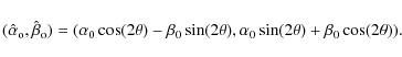
Depending on the orientation we give to the axis of the doublet with respect to the axis of the second doublet, the wavefront can therefore be flipped in various ways. We call the angle between the two axes $\theta$ . If the axes are parallel to each other, i.e. $\theta = 0$ , the wavefront is flipped twice and the wavefront has the same orientation as at the entrance. Then, the on-axis and any off-axis source are extinguished in the image plane by destrutive interference. If the axis of the cylindrical doublets are perpendicular, $\theta = 90^\circ$ , the wavefront is rotated by 180 $^\circ$ as in the AIC configuration, and the ambiguity remains.

In the following, we discuss how setting $\theta$ at values between 0 and 90 $^\circ$ removes the ambiguity of the AIC.

3 The APIC analytical expressions

Here we develop the analytical expressions of the complex amplitudes of the light at the exit of each path for on and off-axis sources in the recombining plane $P_{\rm {R}}$ defined in Fig. 1.

3.1 On-axis source

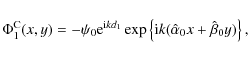
The complex amplitudes of a wavefront propagating path 1 and path 2, the lengths of which are denoted by d₁ and d₂, respectively, are (Goodman 1992):

$\begin{displaymath}\Phi_1^{\rm {S}}(x,y)= -\psi_0 {\rm e}^{{\rm i}kd_1}, \mbox{ for path 1 and } \end{displaymath}$

(1)

$\begin{displaymath}\Phi_2^{\rm {S}}(x,y)= \psi_0 {\rm e}^{{\rm i}kd_2},\mbox{ for path 2,} \end{displaymath}$

(2)

where the superscript S represents the star and the subscripts 1 and 2 designate the path. The $-\pi$ phase shift of the two consecutive cylindrical doublets is considered by the minus sign in Eq. (1).

Thus, in the recombining plane $P_{\rm {R}}$ , as soon as d₁ and d₂ are equal, the sum of the two complex amplitudes for an on-axis source is null.

3.2 Off-axis source

We derive the complex amplitude of an off-axis source located at ( $\alpha _{\rm o},\beta _{\rm o}$ ) in two steps, considering one of the cylindrical lens doublets at a time.

After propagation through the first cylindrical lens doublet with its axis along the y-axis, the complex amplitude becomes

$\begin{displaymath}\Phi_1^{\rm {C}}(x,y)=\psi_0 {\rm e}^{-{\rm i}\frac{\pi}{2}} \exp\left\{{\rm i}k (-\alpha_0 x+\beta_0 y)\right\}\!. \end{displaymath}$

(3)

After going through the second cylindrical lens doublet - rotated by $\theta$ with respect to the first doublet - the coordinates of the wave vector in the previous equation $(-\alpha_{\rm o}, \beta_{\rm o})$ are transformed into $(\hat{\alpha}_{\rm o}, \hat{\beta}_{\rm o})$

$\begin{displaymath}(\hat{\alpha}_{\rm o}, \hat{\beta}_{\rm o})=(\alpha_0 \cos(2\... ...0 \sin(2\theta),\alpha_0 \sin(2\theta) +\beta_0\cos(2\theta)). \end{displaymath}$

(4)

The complex amplitude of the outgoing wavefront becomes

$\begin{displaymath}\Phi_1^{\rm {C}}(x,y)=-\psi_0 {\rm e}^{{\rm i} kd_1} \exp\left\{{\rm i}k (\hat{\alpha}_0 x+\hat{\beta}_0 y)\right\}, \end{displaymath}$

(5)

where the sign minus represents the total phase shift of $-\pi$ affecting the wavefront.

The complex amplitude of a wavefront propagating over path 2 is:

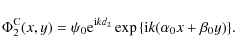
$\begin{displaymath}\Phi^{\rm {C}}_2(x,y)=\psi_0{\rm e}^{{\rm i}kd_2}\exp\left\{{\rm i}k (\alpha_0 x+\beta_0 y)\right\}\!. \end{displaymath}$

(6)

And therefore the sum of both amplitudes in $P_{\rm {R}}$ , assuming d₁=d₂, is

$\begin{displaymath}\Phi^{\rm {C}}(x,y) = \Phi_1^{\rm {C}}+\Phi_2^{\rm {C}} = \ps... ...\rm e}^{{\rm i}k (\hat{\alpha}_0 x +\hat{\beta}_0 y)}\right\}. \end{displaymath}$

(7)

3.3 Complex amplitude and intensity in the image plane

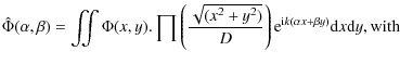
The expression of the complex amplitude in the image plane is given by

$\displaystyle \hat\Phi(\alpha,\beta)=\iint\Phi(x,y).\prod\left(\frac{\sqrt{(x^2... ...D}\right) \mbox{e}^{ {\rm i}k (\alpha x+\beta y)} {\rm d}x{\rm d}y, \mbox{with}$

$\alpha$ and $\beta$ the angular coordinates of a running point in the focal plane;
$\Phi(x,y)$ the complex amplitude in the recombining plane $P_{\rm {R}}$ , the entrance of the recombining lens;
$\prod$ the circular aperture of diameter D;
$\lambda$ the wavelength.

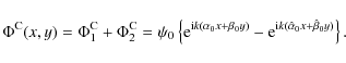
For an off-axis source, the complex amplitude in the image plane is the sum of the Fourier transforms of both complex amplitudes $\Phi_1^{\rm {C}}$ and $\Phi_2^{\rm {C}}$ , from path 1 and path 2 given by Eqs. (3) and (6) respectively:

$\begin{displaymath}\hat{\Phi}^{\rm {C}}_1( \alpha,\beta)=-\frac{\mbox{Cst}}{{\rm... ...}\right)\ast\delta(\alpha-\hat{\alpha}_0,\beta-\hat{\beta}_0), \end{displaymath}$

(8)

$\begin{displaymath}\hat{\Phi}^{\rm {C}}_2(\alpha,\beta)=\frac{\rm {Cst}}{{\rm i}... ...2}}{\lambda }\right)\ast\delta(\alpha-\alpha_0,\beta-\beta_0), \end{displaymath}$

(9)

where $\ast$ denotes the convolution product, Besinc $(x)=2{\rm J}_{\rm 1}(x)/x$ , with J₁ the first-order Bessel function and $\delta(x)$ the Dirac function. The Cst term in the three previous equations covers all the transmission and reflection coefficients induced by the beam splitters and the mirrors. It is assumed equal for the two paths so dismissed in the following.

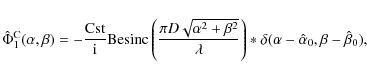
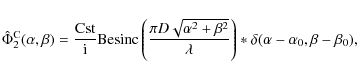
The image intensity distribution $I(\alpha,\beta)$ is given by the squared modulus of the sum of the complex amplitudes,

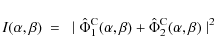
$\begin{displaymath} I(\alpha,\beta) ~=~ \mid \hat{\Phi}^{\rm {C}}_1(\alpha,\beta)+ \hat{\Phi}^{\rm {C}}_2(\alpha,\beta) \mid^2 \end{displaymath}$

$\begin{displaymath}\quad=~\mid \hat{\Phi}^{\rm {C}}_1(\alpha,\beta) \!\mid^2+\mi... ...}}_1(\alpha,\beta)\bar{\hat{\Phi}}^{\rm {C}}_2(\alpha,\beta)], \end{displaymath}$

(10)

where the mixed term, the real part of the complex amplitude product is an interference term.

According to the distance between the two $\delta$ -functions (Eqs. (8) and (9)) the interference is more or less destructive. If this distance is greater than the Rayleigh limit, the two Besinc functions do not overlap and the mixed term is negligible. Then, the total intensity is the sum of two well-separated Airy disks, one centred on $(\hat{\alpha}_{\rm o}, \hat{\beta}_{\rm o})$ and the other on $(\alpha_{\rm o},\beta_{\rm o})$ (Eq. 10).

If the distance is smaller than the Rayleigh limit, the interference term is not negligible and the $\pi$ -dephased Besinc functions will add. Because of this interference, the maximum, or the centre of each Airy disk will be displaced. This point is further discussed in Sect. 4.2.

3.4 Extinction lobe or finding the optimal value for $\theta$

Interferential coronagraphs differ from Lyot-types by their close sensing capability i.e. their ability to detect sources at small separation. This capability can be appreciated through the plot of the extinction lobe of the instrument. The extinction lobe $\omega (\alpha _0,\beta _0)$ , as defined in Baudoz et al. (2000), is given by the integration, in the image plane, of the energy coming from an off-axis source:

$\begin{displaymath} \omega(\alpha_0,\beta_0)=\iint I^{\rm {C}}(\alpha,\beta)\mbox{d}\alpha \mbox{d}\beta. \end{displaymath}$

(11)

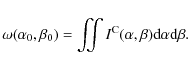
The extinction lobe of our instrument is a function of $\theta$ . Therefore, one way of deducing the most suitable values for $\theta$ is to derive them from the most narrow extinction lobe whose width is defined by its first maximum. In Fig. 2 we see that as $\theta$ increases the extinction lobe narrows down. Numerically we find that all values of $\theta$ ranging between 45¡ and 90¡ are suitable in the sense that they provide an extinction lobe narrower than the Airy lobe of the telescope effectively used. However, this last value of $\theta$ , 90¡, converts APIC into an AIC (i.e., the ambiguity becomes impossible to remove).

This is intuitively understandable considering that for $\theta = 0^\circ$ the two Airy disks are on top of each other, while for increasing $\theta$ they are driven further apart until they end up at opposite sides of the optical axis for $\theta = 90^\circ$ . The latter case permits the smallest separation $(\alpha_0,\beta_0)$ of the off-axis source resulting in the narrowest extinction lobe.

$\begin{figure} \par\includegraphics[height=2.3in,width=3in]{1232fig2.eps}\par\end{figure}$	Figure 2: The extinction lobe $\omega (\alpha _0,\beta _0)$ for different values of $\theta$ . The dotted line represents the extinction lobe of the instrument as a function of the angular coordinate taken in units of 1.22 $\lambda /D$ . The normalized Airy lobe of the telescope is given for comparaison by the solid line. The dashed line limits the Airy radius.
Open with DEXTER

4 Numerical computations

In this secton, we present numerical computations of the intensity distribution for different values of $\theta$ , $\alpha_0$ , and $\beta_0$ and investigate methods for retrieving the planet position on the sky. For our numerical computations, we assumed the following values:

$\lambda$ , the wavelength: 2.2 $\mu$ m;
D, the telescope diameter: 10 m;
intensity ratio between the star and its companion: 10^-6.

$\begin{figure} \par\includegraphics[height=3.5in]{1232fig3.eps} %\end{figure}$	Figure 3: Computed intensity distributions of an off-axis source at position ( $\alpha _{\rm o},\beta _{\rm o}$ ). The values of $\theta$ and ( $\alpha _{\rm o}$ , $\beta _{\rm o}$ ) in milli arcsec are illustrated in the table above. On this colour scale, the on-axis source is invisible.
Open with DEXTER

Although the intensity distributions in Fig. 3 are not symmetrical, it is not obvious which of the two Airy disks represents the true position of the off-axis source. The two sections (Sects. 4.1 and 4.2) are dedicated to retrieving the off-axis position both for images with interference and images without interference (see Eq. (3.3)).

We would like to point out that, in the case of images of low signal-to-noise ratio or having a field crowded with speckles (for example noisy imaging of an extended disk with embedded planets), a more powerful deconvolution routine that takes the known PSF behavior of APIC into account could be used instead of our algorithms developed below.

4.1 Finding the planet from non-interfering subimages

We consider here the separation of the two subimages to be greater than the Rayleigh limit so that the subimages do not interfere.

$\begin{figure} \par\includegraphics[height=1.4in,width=3.6in]{1232fig4.eps} \end{figure}$	Figure 4: On the left, the intensity distribution in the image plane, using the same parameters as in Fig. 3A. In the middle and on the right, computed intensity distributions are displayed if the source were in position P₁ or in P₂.
Open with DEXTER

To find out which of the two Airy disks in Fig. 4 represents the true position of the off-axis source, we computed the intensity distribution first assuming that P₁ in Fig. 4 is the true position, and then that P₂ is correct. The intensity distributions in Fig. 4 demonstrates unambiguously that P₂ is the true position of the off-axis source.

4.2 Finding the planet from interfering subimages

As discussed in Sect. 3.2, if the distance between on- and off-axis source approaches the Rayleigh limit, the two Besinc functions interfere and the resulting intensity distributions show two slightly deformed Airy disks displayed in (Fig. 5). On the right hand side of the same figure, a 1-D cut through the image is shown.

While we can use the same reasoning as in the interference-free case to determine the true position of the off-axis source, the distance $(\alpha_0,\beta_0)$ cannot be measured directly in the image since the local maxima deviate from the real maxima of each (interference-free) Airy disk as illustrated in (Fig. 5). Applying the knowledge of the form of the Airy disk, this effect can be calibrated. Computing the average of several images with varying $\theta$ further reduces the remaining error over the distance $(\alpha_{\rm o},\beta_{\rm o})$ .

5 Discussion and perspectives

In this Research Note, we present the concept of the APIC for the ambiguity removal of the AIC. In addition to the numerical computations, a laboratory test bench was set up to validate the concept and to visualize the motion of the off-axis source in the image plane as a function of the angle $\theta$ between the axes of the two cylindrical doublets. This experiment has shown accurate results for the geometrical optics, matching the theoretical study and the numerical computations.

The interferometric extinction of the on-axis source uses the same principle and has the same restrictions in terms of signal-to-noise and tolerances as the AIC concept presented by Baudoz et al. (2000). We specifically look into the effect of the chromaticity of cylindrical lenses in future experiments determining the potential practical restrictions of a design with lenses.

$\begin{figure} \par\includegraphics[height=1.47in, width=3.5in]{1232fig5.eps} \end{figure}$

Figure 5:

On the left, the image of an off-axis source located below the instrument's resolution, using the same parameters as in Fig. 3D. The interference of the Besinc functions results in a slight deformation of the Airy disks. The straight black line indicates the position of the 1-D cut displayed on the right. Here, the solid line is the intensity distribution formed by two deformed Airy disks. The theoretical form of the interference-free Airy disks at these locations are shown by dashed lines.

Open with DEXTER

6 Conclusion

The concept of APIC lies in the modification of the achromatic interfero-coronagraph (AIC), determining unambiguously the position of a faint companion with respect to its bright parent star. The conceptual modification consists in replacing the cat's eye by two cylindrical lens doublets in one arm of a Mach-Zehnder interferometer. Depending on the rotation angles of the cylindrical doublets, the original axis of symmetry of the AIC is removed and the true position of the faint companion in the sky can be derived from the position of the two images in APIC. This has been studied for different sets of rotation angles, and a few numerical examples have been discussed.

Acknowledgements

We are indebted to J. Gay for discussions of the AIC and APIC concept in general, and for having stimulated more detailed studies of the above-presented concept.

References

Baudoz P., Rabbia Y., & Gay J. 2000, A&AS, 141, 319 [NASA ADS] [CrossRef] [EDP Sciences] (In the text)
Gay J., & Rabbia Y. 1996, C.R. Acad. Sci. Paris. Ser. IIB: Mec. Phys. Chim. Astron., 322, 265 [NASA ADS]
Gouy C. 1892, C.R. Acad. Sci. Paris, 110, 1251 (In the text)
Guyon, O., Pulzhnik, E., Kuchner, M., Collins, B., & Ridgway, S. 2006, ApJS, 167, 81 [NASA ADS] [CrossRef] (In the text)
Goodman J. W. 1992, Statistical Optics (New York: Wiley) (In the text)
Kraus, S., Balega, Y. Y., Berger, J.-P., et al. 2007, A&A, 466, 649 [NASA ADS] [CrossRef] [EDP Sciences] (In the text)
Patience, J., Zavala, R. T., Prato, L., et al. 2008, ApJ, 674, L97 [NASA ADS] [CrossRef] (In the text)
Schöller, M. 2008, private communication (In the text)

Footnotes

... AIC: Called CIA, Coronographe Interferential Achromatique in its original quoting by Gay & Y. Rabbia (1996).
... doublets: By doublet we refer to a pair of identical lenses, thus having the same diameter and the same focal length. They are placed in such a way that the image focus of the first coincides with the object focus of the second.
... doublet: Each cylindrical lens has its own axis, but in each one of our doublets, the two lenses axis are parallel to each other. So from now on we will talk about the one axis of the whole doublet.

All Figures

$\begin{figure} \par\includegraphics[height=2.3in,width=3.5in]{1232fig1.eps}\end{figure}$	Figure 1: The basic design of APIC is a Mach-Zehnder interferometer. Two cylindrical lens doublets, D₁ and D₂, in one arm of the interferometer replace the AIC's cat's eye. The image is formed in the focal plane of a recombining lens, the image plane of APIC. The axes of all the cylindrical lenses in this schematic figure are perpendicular to the paper plane, i.e. parallel to the y-axis of the laboratory.
Open with DEXTER
In the text

$\begin{figure} \par\includegraphics[height=2.3in,width=3in]{1232fig2.eps}\par\end{figure}$	Figure 2: The extinction lobe $\omega (\alpha _0,\beta _0)$ for different values of $\theta$ . The dotted line represents the extinction lobe of the instrument as a function of the angular coordinate taken in units of 1.22 $\lambda /D$ . The normalized Airy lobe of the telescope is given for comparaison by the solid line. The dashed line limits the Airy radius.
Open with DEXTER
In the text

$\begin{figure} \par\includegraphics[height=3.5in]{1232fig3.eps} %\end{figure}$	Figure 3: Computed intensity distributions of an off-axis source at position ( $\alpha _{\rm o},\beta _{\rm o}$ ). The values of $\theta$ and ( $\alpha _{\rm o}$ , $\beta _{\rm o}$ ) in milli arcsec are illustrated in the table above. On this colour scale, the on-axis source is invisible.
Open with DEXTER
In the text

$\begin{figure} \par\includegraphics[height=1.4in,width=3.6in]{1232fig4.eps} \end{figure}$	Figure 4: On the left, the intensity distribution in the image plane, using the same parameters as in Fig. 3A. In the middle and on the right, computed intensity distributions are displayed if the source were in position P₁ or in P₂.
Open with DEXTER
In the text

$\begin{figure} \par\includegraphics[height=1.47in, width=3.5in]{1232fig5.eps} \end{figure}$	Figure 5: On the left, the image of an off-axis source located below the instrument's resolution, using the same parameters as in Fig. 3D. The interference of the Besinc functions results in a slight deformation of the Airy disks. The straight black line indicates the position of the 1-D cut displayed on the right. Here, the solid line is the intensity distribution formed by two deformed Airy disks. The theoretical form of the interference-free Airy disks at these locations are shown by dashed lines.
Open with DEXTER
In the text

Current usage metrics show cumulative count of Article Views (full-text article views including HTML views, PDF and ePub downloads, according to the available data) and Abstracts Views on Vision4Press platform.

Data correspond to usage on the plateform after 2015. The current usage metrics is available 48-96 hours after online publication and is updated daily on week days.

Initial download of the metrics may take a while.

APIC(Research Note)