| Issue |
A&A
Volume 500, Number 3, June IV 2009
|
|
|---|---|---|
| Page(s) | 1271 - 1276 | |
| Section | Astronomical instrumentation | |
| DOI | https://doi.org/10.1051/0004-6361/200811119 | |
| Published online | 16 April 2009 | |
First single star scidar measurements at Dome C, Antarctica
J. Vernin - M. Chadid - E. Aristidi - A. Agabi - H. Trinquet - M. Van der Swaelmen
Laboratoire H. Fizeau, UMR6525, Université de Nice, Observatoire de la Côte d'Azur, Parc Valrose, 06108 Nice - France
Received 9 October 2008 / Accepted 30 January 2009
Abstract
Aims. We investigate the first operational running of the Single Star Scidar (SSS instrument) under harsh weather conditions at Dome C in Antarctica and examine continuous monitoring of the optical turbulence and wind speed profiles throughout the atmosphere.
Methods. SSS is mainly composed of commercially available light-weight components and a 16 inch telescope installed on an equatorial mount. Scintillation patterns were computed (auto and cross-correlations) in real time and analyzed off line to retrieve continuously vertical profiles of optical turbulence CN2(h) and wind speed V(h), from the ground up to 20 km.
Results. Using a simulated annealing method, we have analyzed about 6.5 h of observations, revealing the strong surface layer contribution to seeing degradation. SSS results show a good seeing agreement with simultaneous measurements with a Differential Image Motion Monitor, even under very good seeing as low as 0.2 arcsec, as well as wind speed agreement when compared to the weather archive from NOAA.
Conclusions. SSS has shown its usefulness for site characterization since it simultaneously measures CN2 and V profiles, from which most adaptative optic parameters are deduced, such as isoplanatic angle and coherence time of the wavefront. Due to its small size, it is well adapted for site characterization, even when low infrastructure is available.
Key words: atmospheric effects - site testing - turbulence - instrumentation: detectors - methods: data analysis - methods: observational
1 Introduction
Vernin et al. (2007) gave a brief history of site testing at Dome C, located on the high Antarctica plateau. Studies began in 1992, with a congress (Vernin 1994) organized by the French Académie des Sciences, and soon the decision was taken to begin a two-year site testing campaign at the South Pole. Marks et al. (1999) showed that most of the optical turbulence came from the 200 m boundary layer (BL) triggered by katabatic winds and this motivated the site testing campaign at Dome C where less katabatic winds were expected.
In 1995, one of us, Jean Vernin, participated in the first scientific expedition
to Dome C, but at that time no winter infrastructure was available. In 2005, the Astro-Concordia
station was first opened for winterover during which two DIMMs were set up and
40 meteorological balloons, instrumented for CN2(h) and
![]() profiling, were launched. Again, it became obvious that most of the turbulence was generated within the surface
layer (Agabi et al. 2006), as was found at the South Pole, but with a depth of only 30 m.
profiling, were launched. Again, it became obvious that most of the turbulence was generated within the surface
layer (Agabi et al. 2006), as was found at the South Pole, but with a depth of only 30 m.
There are very few instruments which are able to simultaneously retrieve CN2(h) and
![]() profiles from the ground level up to
profiles from the ground level up to
![]() km where the optical turbulence begins
to be negligible. To our knowledge, only
the Scidar family, i.e.the double star scidar (Vernin & Azouit 1983b,a) and the single star scidar
(Habib et al. 2006) and the instrumented balloon (Azouit & Vernin 2005) are
among these sound techniques.
The Multi Aperture
Scintillation Sensor (Kornilov et al. 2003) or MASS, delivers CN2 profiles along six slabs in the atmosphere, but
it does not give access to ground turbulence nor the wind speed at any altitude. Echo soundings (SODAR) are not
well calibrated in terms of CN2 since they require extra knowledge of the humidity
profile, and their altitude range is around
km where the optical turbulence begins
to be negligible. To our knowledge, only
the Scidar family, i.e.the double star scidar (Vernin & Azouit 1983b,a) and the single star scidar
(Habib et al. 2006) and the instrumented balloon (Azouit & Vernin 2005) are
among these sound techniques.
The Multi Aperture
Scintillation Sensor (Kornilov et al. 2003) or MASS, delivers CN2 profiles along six slabs in the atmosphere, but
it does not give access to ground turbulence nor the wind speed at any altitude. Echo soundings (SODAR) are not
well calibrated in terms of CN2 since they require extra knowledge of the humidity
profile, and their altitude range is around
![]() ,
which may have a serious impact
on site testing (Lawrence et al. 2004). SLODAR (Wilson 2002), based upon wavefront slope analysis on a double star, delivers
optical turbulent profiles. To our knowledge, there are no cross calibrations of the
SLODAR with other techniques or profiles of the wind speed.
,
which may have a serious impact
on site testing (Lawrence et al. 2004). SLODAR (Wilson 2002), based upon wavefront slope analysis on a double star, delivers
optical turbulent profiles. To our knowledge, there are no cross calibrations of the
SLODAR with other techniques or profiles of the wind speed.
Double Star Scidar requires at least a 1 to 1.5 m telescope since it uses a triangulation
method and the maximum reachable altitude
![]() is related to the
diameter D of the entrance
pupil through
is related to the
diameter D of the entrance
pupil through
![]() ,
where
,
where ![]() is the angular separation of the double star. If
one want to probe the atmosphere up to 20-25 km with double stars separated by 4-10 arcsec, such a
telescope is needed. The same argument applies also to the SLODAR technique. Instrumented balloons require a
great deal of ground infrastructure for balloon preparation, balloon launching and then for data reception, but
they can be operated even at new sites where no telescope is available. Thus, for the purpose of
investigation of new modern astronomical site one needs a light-weight experimental setup such as the Single Star Scidar, because it only requires a ``small'' 40 cm telescope.
is the angular separation of the double star. If
one want to probe the atmosphere up to 20-25 km with double stars separated by 4-10 arcsec, such a
telescope is needed. The same argument applies also to the SLODAR technique. Instrumented balloons require a
great deal of ground infrastructure for balloon preparation, balloon launching and then for data reception, but
they can be operated even at new sites where no telescope is available. Thus, for the purpose of
investigation of new modern astronomical site one needs a light-weight experimental setup such as the Single Star Scidar, because it only requires a ``small'' 40 cm telescope.
Here we present the first results obtained at Dome C in 2006 during the second polar winter. In Sect. 2 we present the instrument which was prepared to resist polar conditions. In Sect. 3 we detail the campaign of observations and in Sect. 4 the Single Star Scidar (SSS) results. In Sect. 5 the results are discussed and compared to other sources like DIMM and meteorological re-analysis from the National Oceanic and Atmospheric Administration (NOAA).
2 Instrument
As seen in Fig. 1, the SSS is made with standard components. The telescope is based on a Meade M 16
(40 cm diameter) Ritchey Chrétien optical combination supported by an Astro-Physics 1200 equatorial
mount. At the focus of the telescope, a collimating lens makes the beam parallel, as seen
in the optical scheme in Fig. 2. In order to make the low altitude layers
scintillate, one uses the ``generalized '' scidar mode (Fuchs et al. 1998) in which displacing the photoelectric
receiver by a distance ![]() along the optical axis, one introduces an extra altitude difference
along the optical axis, one introduces an extra altitude difference
![]() ,
where
,
where
![]() is the optical magnification.
is the optical magnification.
The photoelectric receiver is a Pixelfly CCD with a fast readout of
![]() images per second and a low readout noise
(
images per second and a low readout noise
(
![]() ). Auto-correlations and cross-correlations between images separated by
a temporal lag
). Auto-correlations and cross-correlations between images separated by
a temporal lag
![]() ,
,
![]() and
and
![]() ms are computed in real time
and averaged over
ms are computed in real time
and averaged over ![]() images.
In order to disentangle the broadening effect of the altitude and the
wind velocity fluctuations during the time to process the N images, two cross-correlations are necessary (more details are found in Habib et al. 2006).
images.
In order to disentangle the broadening effect of the altitude and the
wind velocity fluctuations during the time to process the N images, two cross-correlations are necessary (more details are found in Habib et al. 2006).
![\begin{figure}
\par\includegraphics[width=9cm]{1119fig1}
\end{figure}](/articles/aa/full_html/2009/24/aa11119-08/img29.png) |
Figure 1: Installation of the SSS above one of the two plateforms at Dome C during polar summer 2005-2006. |
| Open with DEXTER | |
2.1 CN2 and V retrieval
To retrieve the respective vertical profiles of Cn2(h),
![]() and
and
![]() (the variance of wind speed fluctuations at altitude h), we use
a ``Simulated Annealing'' (SA) algorithm which is also described in Habib et al. (2006). Here,
we recall only that altitudes are sampled from 0 to 20 km, with a 1 km vertical resolution which
is about the natural vertical resolution of the SSS. Since the surface layer,
(the variance of wind speed fluctuations at altitude h), we use
a ``Simulated Annealing'' (SA) algorithm which is also described in Habib et al. (2006). Here,
we recall only that altitudes are sampled from 0 to 20 km, with a 1 km vertical resolution which
is about the natural vertical resolution of the SSS. Since the surface layer,
![]() thick,
is very turbulent (Trinquet et al. 2008) we gave the SA algorithm the possibility
of reconstructing four turbulent layers all situated at zero altitude, but with different
wind speed components
thick,
is very turbulent (Trinquet et al. 2008) we gave the SA algorithm the possibility
of reconstructing four turbulent layers all situated at zero altitude, but with different
wind speed components
![]() .
Knowing that the wind speed is increasing with altitude in the Ekman layer,
we sorted these four layers according to
increasing wind speed. Above this surface layer, the first reconstructed altitude is
1 km and then 2 km, 3 km up to 20 km. If the refractive index
structure constant is less than some threshold (
CN2 < 10-18 m-2/3), we assume that there is
not enough turbulence to detect it and to assess its velocity. When the wind speed is zero in the first slab of the four boundary turbulent layers, it is assumed that turbulence is relevant to ``mirror seeing'' and is removed from our analysis,
as already discussed by Avila et al. (2001). An ambiguity might remain if the velocity
of a boundary turbulent layer is less than the first detectable speed
.
Knowing that the wind speed is increasing with altitude in the Ekman layer,
we sorted these four layers according to
increasing wind speed. Above this surface layer, the first reconstructed altitude is
1 km and then 2 km, 3 km up to 20 km. If the refractive index
structure constant is less than some threshold (
CN2 < 10-18 m-2/3), we assume that there is
not enough turbulence to detect it and to assess its velocity. When the wind speed is zero in the first slab of the four boundary turbulent layers, it is assumed that turbulence is relevant to ``mirror seeing'' and is removed from our analysis,
as already discussed by Avila et al. (2001). An ambiguity might remain if the velocity
of a boundary turbulent layer is less than the first detectable speed ![]() given by:
given by:
 |
(1) |
where
Six minutes of CPU time are required to compute vertical profiles of CN2, ![]() and
and
![]() deduced from the auto and cross-correlations averaged over a set of 2000 images, corresponding
to an acquisition time of about 14 s. This means that 180 h, i.e. one week, of CPU
(Opteron processor) time is required to
process 6 h of observations.
deduced from the auto and cross-correlations averaged over a set of 2000 images, corresponding
to an acquisition time of about 14 s. This means that 180 h, i.e. one week, of CPU
(Opteron processor) time is required to
process 6 h of observations.
| |
Figure 2:
Principle of the generalized SSS. After passing through the telescope, light is collimated by
a short focal lens. In order to make the low altitude layers scintillate, the photoelectric
receiver is displaced by a distance |
| Open with DEXTER | |
2.2 SSS detectivity
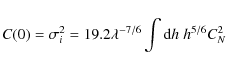
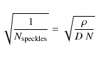
The detectivity of the SSS depends on the noise in the scintillation auto and cross-correlations. As expressed by Vernin & Azouit (1983b), the relative error on the correlation function is given by: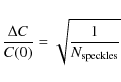
where
 |
(3) |
and
 |
(4) |
where
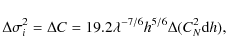 |
(5) |
one can relate the SSS detectivity
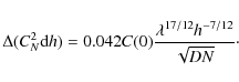
This result allows us to determine the absolute error on the CN2(h) profile and which will be used later in the text.
3 Observations at Dome C in 2006
3.1 Description of the observing campaign
The SSS instrument was designed and constructed in our laboratory and sent to Dome C, Antarctica, lat.Observations began in March 2006, ending in September of the same year. For the reason explained in Sect. 2, we present here only one observing ``night'', on 20 March 2006, of 6.5 h with comparisons to other types of measurements.
3.2 C
N2(h), V(h) and
 (h) profiles deduced from scintillation auto
and cross-correlations
(h) profiles deduced from scintillation auto
and cross-correlations
In Fig. 3, from left to right, an auto-correlation of the scintillation
moving pattern and the first and second cross-correlations, taken respectively at
![]() ms and
14 ms, are visible. In the second cross-correlation, several bumps are detected, each one corresponding to
a different turbulent layer. In Fig. 4, the same cross-correlation
computed at
ms and
14 ms, are visible. In the second cross-correlation, several bumps are detected, each one corresponding to
a different turbulent layer. In Fig. 4, the same cross-correlation
computed at
![]() ms, as in Fig. 3, and the theoretical reconstructed
cross-correlation at the end of the SA process have been plotted. All the bumps corresponding to
different turbulent layers are well detected.
ms, as in Fig. 3, and the theoretical reconstructed
cross-correlation at the end of the SA process have been plotted. All the bumps corresponding to
different turbulent layers are well detected.
| |
Figure 3:
From left to right, two-dimensional auto-correlation, first and second cross-correlation of the scintillation pattern on the 40 cm entrance pupil of the telescope
corresponding to time lags |
| Open with DEXTER | |
![\begin{figure}
\par\includegraphics[width=9cm]{1119fig4}
\end{figure}](/articles/aa/full_html/2009/24/aa11119-08/img52.png) |
Figure 4:
Measured temporal cross-correlation ( left) at |
| Open with DEXTER | |
![\begin{figure}
\par\includegraphics[angle=270,width=18cm]{1119fig5}
\end{figure}](/articles/aa/full_html/2009/24/aa11119-08/img55.png) |
Figure 5:
Top left: median vertical profile of the optical turbulence on a logarithmic
scale CN2(h)and
|
| Open with DEXTER | |
4 Results
In Fig. 5 top panel, we present the mean vertical profiles averaged over the whole ``night''
of 20 March. For clarity, the four first layers at zero altitude have been averaged. Almost all the optical turbulence
is concentrated within the surface layer, the rest being scattered through the free atmosphere, as
reported by Trinquet et al. (2008). The dash-dotted line represents the detectivity
of the SSS, as deduced from Eq. (6), with C(0)=0.1,
N = 2000,
![]() km and D = 0.4 m, which correspond to the observing conditions during this night.
Close to the BL, the detectivity is about
km and D = 0.4 m, which correspond to the observing conditions during this night.
Close to the BL, the detectivity is about
![]() ,
and less than 10-18 above,
in accordance with the threshold given in Sect. 2.1.
,
and less than 10-18 above,
in accordance with the threshold given in Sect. 2.1.
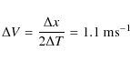
The wind speed, which corresponds to turbulent slabs, increases from ice level to reach 13 ms-1 at 8 km and remains stable above.
In Fig. 6, the temporal evolution of CN2(h) (top)
and
![]() (bottom) profiles during the same night are shown. For clarity, the free atmosphere
and surface layer are plotted separately, one on top and the other at the bottom of
each sub-figure. The first colored line, corresponding to a [0-1] km slab, refers to the
average of the four turbulent slabs which are detailed below. It is clear again that most
of the OT is concentrated within the surface layer, and that the free atmosphere is
quite stable.
(bottom) profiles during the same night are shown. For clarity, the free atmosphere
and surface layer are plotted separately, one on top and the other at the bottom of
each sub-figure. The first colored line, corresponding to a [0-1] km slab, refers to the
average of the four turbulent slabs which are detailed below. It is clear again that most
of the OT is concentrated within the surface layer, and that the free atmosphere is
quite stable.
Trinquet et al. (2008) & Roddier (1981) showed that, from the knowledge of both CN2(h)
and
![]() ,
one can compute
the seeing
,
one can compute
the seeing
![]() ,
the isoplanatic angle for adaptive optics
,
the isoplanatic angle for adaptive optics ![]() and
the coherence time
and
the coherence time ![]() for adaptive optics.
for adaptive optics.
It is clear that the greater r0, ![]() and
and ![]() ,
the better the conditions
for adaptive optics or interferometry. A more general approach is given by Lloyd (2004).
He defines a ``coherence étendue'' G0in which a photon remains coherent and which takes into account
a combination of Fried's radius, isoplanatic
angle and coherence time:
,
the better the conditions
for adaptive optics or interferometry. A more general approach is given by Lloyd (2004).
He defines a ``coherence étendue'' G0in which a photon remains coherent and which takes into account
a combination of Fried's radius, isoplanatic
angle and coherence time:

This new formulation shows a strong dependency on r0 and
From Fig. 7, one notes that the three variables, seeing, isoplanatic angle and coherence time vary on small time scales and with large amplitude.
![\begin{figure}
\par\includegraphics[angle=270,width=9cm]{1119fig6a}
\includegraphics[angle=270,width=9cm]{1119fig6b}
\end{figure}](/articles/aa/full_html/2009/24/aa11119-08/img60.png) |
Figure 6:
Temporal evolution of the optical turbulence
Cn2(h,t) ( top)
and of the wind speed modulus
|
| Open with DEXTER | |
![\begin{figure}
\par\includegraphics[angle=270,width=9cm]{1119fig7}
\end{figure}](/articles/aa/full_html/2009/24/aa11119-08/img61.png) |
Figure 7:
From top left to bottom right: temporal evolution of the
seeing
|
| Open with DEXTER | |
5 Discussion
![\begin{figure}
\par\includegraphics[angle=270,width=9cm]{1119fig8}
\end{figure}](/articles/aa/full_html/2009/24/aa11119-08/img62.png) |
Figure 8: Temporal evolution of seeing measured by SSS (red crosses) and DIMM (line) during 6.5 h on 20 March 2006. |
| Open with DEXTER | |
During the 2006 polar winter a DIMM (Agabi et al. 2006)
was operating on an other platform, 15 m away from the SSS platform, both at 8 m above ice level. The DIMM measures
the seeing continuously and it allows a direct comparison with SSS seeing measurements. In Fig. 8, the temporal
evolution of the seeing as measured by the DIMM (black line) and the SSS (red crosses) are
superimposed. Both instruments are
in very good agreement. From 17:15 to 17:30 some discrepancies are visible which
can be explained by the fact that the distance
between the two experiments, 15 m, is comparable to the thickness of the surface layer,
30 m, which accounts for 80% of the whole optical turbulence (Trinquet et al. 2008).
The overall good agreement means that SSS detects all the turbulent layers in a quantitative way. We recall
that SSS is an ``auto-calibrated'' instrument, where no calibration parameter is introduced.
This is related to the fact that the scintillation variance
![]() is auto-calibrated, by
definition, with the square of the mean flux
is auto-calibrated, by
definition, with the square of the mean flux
![]() .
In
Fig. 9 we plot the DIMM seeing v.s the SSS seeing. The slope of
the line is 0.97 with a 0.75 correlation coefficient. The regression slope is very close
to 1 and seeing amplitude variations of both DIMM and SSS are between 0.2-0.5 and
1.5-1.7 arcsec.The SSS is even able to detect very low turbulence conditions,
as shown in Fig. 10, where
the seeing lies around 0.2-0.3 arcsec.
.
In
Fig. 9 we plot the DIMM seeing v.s the SSS seeing. The slope of
the line is 0.97 with a 0.75 correlation coefficient. The regression slope is very close
to 1 and seeing amplitude variations of both DIMM and SSS are between 0.2-0.5 and
1.5-1.7 arcsec.The SSS is even able to detect very low turbulence conditions,
as shown in Fig. 10, where
the seeing lies around 0.2-0.3 arcsec.
![\begin{figure}
\par\includegraphics[angle=270,width=9cm]{1119fig9}
\end{figure}](/articles/aa/full_html/2009/24/aa11119-08/img65.png) |
Figure 9: Correlation between seeings measured by SSS and DIMM. |
| Open with DEXTER | |
![\begin{figure}
\par\includegraphics[angle=270,width=9cm]{1119fig10}
\end{figure}](/articles/aa/full_html/2009/24/aa11119-08/img66.png) |
Figure 10: Temporal evolution of seeing measured by SSS (red crosses) and DIMM (line) during 0.5 h over 21 March 2006. 0.2 to 0.3 arcsec seeings are detected both by SSS and DIMM. |
| Open with DEXTER | |
In order to check for the validity of the wind speed deduced from SSS measurements,
we used the National Oceanic and
Atmospheric Administration re-analysis which is available on their web site
(http://www.arl.noaa.gov/READYcmet.php). NOAA profiles
are vertically sampled from ground level up to 26 km over 14 levels, starting
at 0 UT, and
every three hours a new
re-analysis is issued. The first level, or Surface Level,
corresponds to ![]() m above ground. In the bottom of Fig. 5, NOAA wind speed
and direction are plotted in green. Excellent agreement!
Fig. 11 gives a comparison of the temporal
evolution of the wind speed deduced from the first four levels of the SSS and the first two levels,
10m (rectangles) and 400 m (triangles) from the NOAA re-analysis. The wind speed at these
two levels are compatible with the second and third SSS levels, at the surface layer.
m above ground. In the bottom of Fig. 5, NOAA wind speed
and direction are plotted in green. Excellent agreement!
Fig. 11 gives a comparison of the temporal
evolution of the wind speed deduced from the first four levels of the SSS and the first two levels,
10m (rectangles) and 400 m (triangles) from the NOAA re-analysis. The wind speed at these
two levels are compatible with the second and third SSS levels, at the surface layer.
![\begin{figure}
\par\includegraphics[angle=270,width=9cm]{1119fig11}
\end{figure}](/articles/aa/full_html/2009/24/aa11119-08/img68.png) |
Figure 11:
Temporal evolution of the wind speed modulus deduced from SSS measurements in the four
layers within the boundary layer, with a one-hour sliding triangle convolution.
The two measurements from NOAA re-analysis at |
| Open with DEXTER | |
6 Conclusion
We have shown that the Single Star Scidar technique is extremely well suited for astronomical site characterization, even under he worst weather conditions on the high Antarctic plateau. The instrument is robust, reliable, well calibrated and allows the access of vertical profiles of both CN2(h) andSSS seeing measurements obtained for 6.5 h on 20 March 2006 are consistent with other optical experiment like DIMM, even under very low turbulence conditions. SSS wind speed profiles are well comparable with NOAA meteorological re-analysis, from the ground up to 25 km. As expected, above the high Antarctica plateau, SSS shows the same optical turbulence distribution, mainly concentrated within the surface layer.
Acknowledgements
We are indebted to the technical staff of Fizeau laboratory for its help in the construction of the SSS prototype. We thank the Institut Paul-Emile Victor personnel as well as the members of Antarctica expedition who helped in the infrastructure at Dome C. The SSS prototype working at Dome C has been funded by the French ``Institut National des Sciences de l'Univers''. National Oceanic and Atmospheric Administration is acknowledged for access to its meteorological re-analysis profiles through its ARL web-site. Part of the development of the SSS technique was undertaken in the framework of the contract #F61775-02-C0002 with the US Air Force EOARD.
References
- Agabi, A., Aristidi, E., Azouit, M., et al. 2006, PASP, 118, 344 [NASA ADS] [CrossRef] (In the text)
- Avila, R., Vernin, J., & Sánchez, L. J. 2001, A&A, 369, 364 [NASA ADS] [CrossRef] [EDP Sciences]
- Azouit, M., & Vernin, J. 2005, PASP, 117, 536 [NASA ADS] [CrossRef] (In the text)
- Fuchs, A., Tallon, M., & Vernin, J. 1998, PASP, 110, 86 [NASA ADS] [CrossRef] (In the text)
- Habib, A., Vernin, J., Benkhaldoun, Z., & Lanteri, H. 2006, MNRAS, 368, 1456 [NASA ADS] [CrossRef] (In the text)
- Kornilov, V., Tokovinin, A. A., Vozyakova, O., et al. 2003, in Adaptive Optical System Technologies II., ed. P. L. Wizinowich, & D. Bonaccini, SPIE, 4839, 837 (In the text)
- Lawrence, J. S., Ashley, M. C. B., Tokovinin, A., & Travouillon, T. 2004, Nature, 431, 278 [NASA ADS] [CrossRef] (In the text)
- Lloyd, J. P. 2004, in New Frontiers in Stellar Interferometry, ed. W. A. Traub, 5491, 190 (In the text)
- Marks, R. D., Vernin, J., Azouit, M., Manigault, J. F., & Clevelin, C. 1999, A&AS, 134, 161 [NASA ADS] [CrossRef] [EDP Sciences]
- Roddier, F. 1981, Prog. Optics, 19, 281 (In the text)
- Trinquet, H., Agabi, A., Vernin, J., et al. 2008, PASP, 120, 203 [NASA ADS] [CrossRef] (In the text)
- Vernin, J. 1994, in Recherches polaires: une stratégie pour l'an 2000, Académie des Sciences (Paris, Tec & Doc, Lavoisier), 91 (In the text)
- Vernin, J., Agabi, A., Aristidi, E., et al. 2007, Highlights of Astronomy, 14, 693 [NASA ADS] (In the text)
- Vernin, J., & Azouit, M. 1983a, Journal d'Optique, 14, 5 [NASA ADS]
- Vernin, J., & Azouit, M. 1983b, Journal d'Optique, 14, 131 [NASA ADS] (In the text)
- Wilson, R. W. 2002, MNRAS, 337, 103 [NASA ADS] [CrossRef] (In the text)
All Figures
| |
Figure 1: Installation of the SSS above one of the two plateforms at Dome C during polar summer 2005-2006. |
| Open with DEXTER | |
| In the text | |
| |
Figure 2:
Principle of the generalized SSS. After passing through the telescope, light is collimated by
a short focal lens. In order to make the low altitude layers scintillate, the photoelectric
receiver is displaced by a distance |
| Open with DEXTER | |
| In the text | |
| |
Figure 3:
From left to right, two-dimensional auto-correlation, first and second cross-correlation of the scintillation pattern on the 40 cm entrance pupil of the telescope
corresponding to time lags |
| Open with DEXTER | |
| In the text | |
| |
Figure 4:
Measured temporal cross-correlation ( left) at |
| Open with DEXTER | |
| In the text | |
| |
Figure 5:
Top left: median vertical profile of the optical turbulence on a logarithmic
scale CN2(h)and
|
| Open with DEXTER | |
| In the text | |
| |
Figure 6:
Temporal evolution of the optical turbulence
Cn2(h,t) ( top)
and of the wind speed modulus
|
| Open with DEXTER | |
| In the text | |
| |
Figure 7:
From top left to bottom right: temporal evolution of the
seeing
|
| Open with DEXTER | |
| In the text | |
| |
Figure 8: Temporal evolution of seeing measured by SSS (red crosses) and DIMM (line) during 6.5 h on 20 March 2006. |
| Open with DEXTER | |
| In the text | |
| |
Figure 9: Correlation between seeings measured by SSS and DIMM. |
| Open with DEXTER | |
| In the text | |
| |
Figure 10: Temporal evolution of seeing measured by SSS (red crosses) and DIMM (line) during 0.5 h over 21 March 2006. 0.2 to 0.3 arcsec seeings are detected both by SSS and DIMM. |
| Open with DEXTER | |
| In the text | |
| |
Figure 11:
Temporal evolution of the wind speed modulus deduced from SSS measurements in the four
layers within the boundary layer, with a one-hour sliding triangle convolution.
The two measurements from NOAA re-analysis at |
| Open with DEXTER | |
| In the text | |
Copyright ESO 2009
Current usage metrics show cumulative count of Article Views (full-text article views including HTML views, PDF and ePub downloads, according to the available data) and Abstracts Views on Vision4Press platform.
Data correspond to usage on the plateform after 2015. The current usage metrics is available 48-96 hours after online publication and is updated daily on week days.
Initial download of the metrics may take a while.