| Issue |
A&A
Volume 500, Number 3, June IV 2009
|
|
|---|---|---|
| Page(s) | 1193 - 1205 | |
| Section | Stellar structure and evolution | |
| DOI | https://doi.org/10.1051/0004-6361/200811060 | |
| Published online | 29 April 2009 | |
High-resolution smoothed particle hydrodynamics simulations of the merger of binary white dwarfs
P. Lorén-Aguilar1,2 - J. Isern3,2 - E. García-Berro1,2
1 - Departament de Física Aplicada,
Escola Politécnica Superior de Castelldefels,
Universitat Politècnica de Catalunya,
Avda. del Canal Olímpic 15,
08860 Castelldefels, Spain
2 -
Institute for Space Studies of Catalonia,
c/Gran Capità 2-4, Edif. Nexus 104,
08034 Barcelona, Spain
3 -
Institut de Ciències de l'Espai, CSIC,
Campus UAB, Facultat de Ciències, Torre C-5,
08193 Bellaterra, Spain
Received 30 September 2008 / Accepted 15 March 2009
Abstract
Context. The coalescence of two white dwarfs is the final outcome of a sizeable fraction of binary stellar systems. Moreover, this process has been proposed to explain several interesting astrophysical phenomena.
Aims. We present the results of a set of high-resolution simulations of the merging process of two white dwarfs.
Methods. We use an up-to-date smoothed particle hydrodynamics code that incorporates very detailed input physics and an improved treatment of the artificial viscosity. Our simulations have been done using a large number of particles (![]()
![]() )
and covering the full range of masses and chemical compositions of the coalescing white dwarfs. We also compare the time evolution of the system during the first phases of the coalescence with what is obtained using a simplified treatment of mass transfer; we discuss in detail the characteristics of the final configuration; we assess the possible observational signatures of the merger, such as the associated gravitational waveforms and the fallback X-ray flares; and we study the long-term evolution of the coalescence.
)
and covering the full range of masses and chemical compositions of the coalescing white dwarfs. We also compare the time evolution of the system during the first phases of the coalescence with what is obtained using a simplified treatment of mass transfer; we discuss in detail the characteristics of the final configuration; we assess the possible observational signatures of the merger, such as the associated gravitational waveforms and the fallback X-ray flares; and we study the long-term evolution of the coalescence.
Results. The mass transfer rates obtained during the first phases of the merger episode agree with the theoretical expectations. In all the cases studied, the merged configuration is a central compact object surrounded by a self-gravitating Keplerian disk, except in the case where two equal-mass white dwarfs coalesce.
Conclusions. We find that the overall evolution the system and the main characteristics of the of the final object agree with other previous studies in which lower resolutions were used. We also find that the fallback X-ray luminosities are close to 1047 erg/s. The gravitational waveforms are characterized by the sudden disappearance of the signal in a few orbital periods.
Key words: stars: white dwarfs - stars: interiors - stars: binaries: close - hydrodynamics - accretion, accretion disks
1 Introduction
The coalescence of two close white dwarfs is thought to be one of the most common endpoints in the evolution of binary systems. Consequently, the coalescence process is an interesting issue with many potential applications. Although the astrophysical scenarios in which the coalescence of two white dwarfs in a close binary system can occur and their relative frequencies have been often studied - see, for instance, Yungelson et al. (1994), Nelemans et al. (2001a,b), and the recent review of Postnov & Yungelson (2006) - the merging process has received little attention until recently. The pioneering works of Mochkovitch & Livio (1989, 1990) who used an approximate method - the so-called self-consistent-field method (Clement 1974) - and the full smoothed particle hydrodynamic (SPH) simulations of Benz et al. (1989a), Benz et al. (1989a), Benz et al. (1989a), Benz et al. (1990), Rasio & Shapiro (1995) and Segretain et al. (1997) were the only exceptions.
Most of these early works had several drawbacks. For instance, some
of them did not include a detailed nuclear network, or else the
network was very simplistic; others used a very small number of SPH
particles (![]() 103) and, finally, others did not discuss the
properties of the merger configuration. Additionally, all these early
works studied a reduced set of masses and chemical compositions and
used the classical expression for the artificial viscosity (Monaghan
& Gingold 1983). This is an important issue since it is well known
that SPH induces a strong shear viscosity, which is more pronounced
when the classical expression for the artificial viscosity is used.
Likewise, energy dissipation by artificial viscosity can lead to
overheating so the peak temperatures achieved during the merger and
the associated nucleosynthesis depend on the choice of the artificial
viscosity. However, the situation changed recently, when Guerrero
et al. (2004) opened the way to more realistic simulations. In these
calculations the standard prescription of Monaghan & Gingold (1983)
for the artificial viscosity was used, but the switch originally
suggested by Balsara (1995) was employed to partially suppress the
excess of dissipation. More recently, the simulations of Yoon et al.
(2007) were carried out using a modern prescription for the artificial
viscosity with time-dependent parameters (Morris & Monaghan 1997),
which guarantees that viscosity is essentially absent in those parts
of the fluid in which it is not necessary, but there are other
prescriptions that are also suitable. In particular, the prescription
of Monaghan (1997), which is based in Riemann-solvers also yields
excellent results, and does not result in overheating. This is the
prescription we use in the present work.
103) and, finally, others did not discuss the
properties of the merger configuration. Additionally, all these early
works studied a reduced set of masses and chemical compositions and
used the classical expression for the artificial viscosity (Monaghan
& Gingold 1983). This is an important issue since it is well known
that SPH induces a strong shear viscosity, which is more pronounced
when the classical expression for the artificial viscosity is used.
Likewise, energy dissipation by artificial viscosity can lead to
overheating so the peak temperatures achieved during the merger and
the associated nucleosynthesis depend on the choice of the artificial
viscosity. However, the situation changed recently, when Guerrero
et al. (2004) opened the way to more realistic simulations. In these
calculations the standard prescription of Monaghan & Gingold (1983)
for the artificial viscosity was used, but the switch originally
suggested by Balsara (1995) was employed to partially suppress the
excess of dissipation. More recently, the simulations of Yoon et al.
(2007) were carried out using a modern prescription for the artificial
viscosity with time-dependent parameters (Morris & Monaghan 1997),
which guarantees that viscosity is essentially absent in those parts
of the fluid in which it is not necessary, but there are other
prescriptions that are also suitable. In particular, the prescription
of Monaghan (1997), which is based in Riemann-solvers also yields
excellent results, and does not result in overheating. This is the
prescription we use in the present work.
It is also interesting to realize that the number of particles used in
these kind of simulations has increased considerably in the last few
years, according to the available computing power. For instance,
Segretain et al. (1997) used ![]()
![]() SPH particles to
simulate the coalescence of a
SPH particles to
simulate the coalescence of a
![]() system. Later,
Guerrero et al. (2004) studied a considerable range of masses and
chemical compositions of the merging white dwarfs employing a sizeable
number of particles (
system. Later,
Guerrero et al. (2004) studied a considerable range of masses and
chemical compositions of the merging white dwarfs employing a sizeable
number of particles (![]()
![]() ). This range of masses and
chemical compositions included 6 runs in which several inital
configurations were studied, involving helium, carbon-oxygen, and
oxygen-neon white dwarfs. Lorén-Aguilar et al. (2005) simulated
the coalescence of a system of two equal-mass carbon-oxygen white
dwarfs of
). This range of masses and
chemical compositions included 6 runs in which several inital
configurations were studied, involving helium, carbon-oxygen, and
oxygen-neon white dwarfs. Lorén-Aguilar et al. (2005) simulated
the coalescence of a system of two equal-mass carbon-oxygen white
dwarfs of
![]() .
However, in this work only one
high-resolution simulation was done. More recently, Yoon et al. (2007)
studied in detail the coalescence of a binary system composed of two
white dwarfs of masses 0.6 and
.
However, in this work only one
high-resolution simulation was done. More recently, Yoon et al. (2007)
studied in detail the coalescence of a binary system composed of two
white dwarfs of masses 0.6 and
![]() using
using
![]() SPH particles. However, only one simulation was presented in this
work. It is thus clear that a thorough parametric study in which
several white dwarf masses and chemical compositions are explored
using a large number of SPH particles and a more elaborate treatment
of the artificial viscosity remains to be done.
SPH particles. However, only one simulation was presented in this
work. It is thus clear that a thorough parametric study in which
several white dwarf masses and chemical compositions are explored
using a large number of SPH particles and a more elaborate treatment
of the artificial viscosity remains to be done.
Possible applications of these kind of simulations include the double-degenerate scenario to account for Type Ia supernova outbursts (Webbink 1984; Iben & Tutukov 1984) and the formation of magnetars (King et al. 2001). Also, three hot and massive white dwarfs members of the Galactic halo could be the result of the coalescence of a double white-dwarf binary system (Schmidt et al. 1992; Segretain et al. 1997). Additionally, hydrogen-deficient carbon and R Corona Borealis stars (Izzard et al. 2007; Clayton et al. 2007) and extreme helium stars (Pandey et al. 2005) are thought to be the consequence of the merging of two white dwarfs. Finally, the large metal abundances found around some hydrogen-rich white dwarfs with dusty disks around them can be explained by the merger of a CO and a He white dwarf (García-Berro et al. 2007). Last but not least, the phase previous to the coalescence of a double white-dwarf close binary system has been shown to be a powerful source of gravitational waves that would be eventually detectable by LISA (Lorén-Aguilar et al. 2005).
Depending on the mass ratio of both stars and on the initial
conditions of the binary system, the fate of double white dwarf binary
systems is a merging process because angular momentum losses through
gravitational wave radiation. Stars orbit each other at decreasing
orbital separations until the less massive one overfills its Roche
lobe and mass transfer begins. According to the initial conditions,
mass transfer proceeds either in a stable or a dynamically unstable
regime. The stability of mass transfer is an important issue. If the
mass transfer process is stable, mass will flow at relatively low
accretion rates, and the whole merging process could last for several
million years. In contrast, if mass transfer proceds in an unstable
way, the whole merging process finishes in a few minutes. The
difference between the two cases relies on the ability of the binary
system to return enough angular momentum back to the orbit. In fact,
there are two competing processes. On the one hand, the donor star is
supported by the pressure of degenerate electrons, so it will expand
as it loses mass, thus enhancing the mass-transfer rate. On the other,
if orbital angular momentum is conserved, the orbit will expand as the
donor star loses mass, thus reducing the mass-transfer rate. The
precise trade-off between both physical processes determines the
stability of mass transfer. Guerrero et al. (2004) find that all the
systems merged in a few hundred seconds, corresponding to mass
transfer rates of ![]()
![]() s-1. Since the
Eddington rate is about
s-1. Since the
Eddington rate is about
![]() yr-1, the most
massive white dwarf cannot incorporate the material of the disrupted
secondary on such a short timescale and, thus, the secondary forms a
hot atmosphere and a heavy Keplerian disk around the primary. This has
been challenged by the simulations of Motl et al. (2002) and
D'Souza et al. (2006). These authors used a grid-based, three-dimensional
finite-difference Eulerian hydrodynamical code and found that mass
transfer is stable when the stars are co-rotating. Nevertheless, it
should be noted that these simulations were done using simplified
physical inputs; for instance, they used a polytropic equation of
state. More importantly, grid-based methods are known to poorly
conserve angular momentum. In either case, it is clear that large
spatial resolutions are required to assess the stability of mass
transfer given the degenerate nature of the donor star, since once
mass transfer begins, the radius of the secondary increases very
rapidly, thereby increasing the mass-loss rate.
yr-1, the most
massive white dwarf cannot incorporate the material of the disrupted
secondary on such a short timescale and, thus, the secondary forms a
hot atmosphere and a heavy Keplerian disk around the primary. This has
been challenged by the simulations of Motl et al. (2002) and
D'Souza et al. (2006). These authors used a grid-based, three-dimensional
finite-difference Eulerian hydrodynamical code and found that mass
transfer is stable when the stars are co-rotating. Nevertheless, it
should be noted that these simulations were done using simplified
physical inputs; for instance, they used a polytropic equation of
state. More importantly, grid-based methods are known to poorly
conserve angular momentum. In either case, it is clear that large
spatial resolutions are required to assess the stability of mass
transfer given the degenerate nature of the donor star, since once
mass transfer begins, the radius of the secondary increases very
rapidly, thereby increasing the mass-loss rate.
In the present paper we study the coalescence of binary white dwarfs
employing an enhanced spatial resolution (
![]() SPH
particles) and a formulation of the artificial viscosity which very
much reduces the excess of shear. The number of particles used in our
simulations is one order of magnitude greater than those used in our
previous simulations (Guerrero et al. 2004) and within a factor
of 2
of those used in modern simulations (Yoon et al. 2007;
Lorén-Aguilar et al. 2005). This allows us to resolve smaller scale
lengths - by a factor
SPH
particles) and a formulation of the artificial viscosity which very
much reduces the excess of shear. The number of particles used in our
simulations is one order of magnitude greater than those used in our
previous simulations (Guerrero et al. 2004) and within a factor
of 2
of those used in modern simulations (Yoon et al. 2007;
Lorén-Aguilar et al. 2005). This allows us to resolve smaller scale
lengths - by a factor
![]() - than in
Guerrero et al. (2004). Moreover, this is done for a broad range of
initial masses and chemical compositions of the coalescing white
dwarfs, in contrast to most modern simulations, in which only a single
coalescence was studied in detail (Yoon et al. 2007). In particular
we study the following cases:
- than in
Guerrero et al. (2004). Moreover, this is done for a broad range of
initial masses and chemical compositions of the coalescing white
dwarfs, in contrast to most modern simulations, in which only a single
coalescence was studied in detail (Yoon et al. 2007). In particular
we study the following cases:
![]() ,
,
![]() ,
,
![]() ,
,
![]() and
and
![]() .
Although we have computed several mergers, we only
discuss in detail the results of the merger of a
.
Although we have computed several mergers, we only
discuss in detail the results of the merger of a
![]() binary system. The main results of the rest of the
simulations are only given in tabular form, but can be provided upon
request. Accordingly, we devote most of the paper to compare the
results of this simulation with those previously available, and we
postpone the discussion of the effects of the initial conditions to a
forthcoming publication. The paper is organized as follows. A
brief description of our SPH code is given in Sect. 2. In
Sect. 3
we describe our results and in Sect. 4 we compare them with those of
other authors. In Sect. 5 we discuss our simulations.
Specifically, we pay special attention to the stability of the mass
transfer episode. This is done in Sect. 5.1, whereas in
Sects. 5.2 and 5.3 the possible observational signatures arising from the
merging process are studied. In particular, we consider the
gravitational wave pattern of the several mergers studied here
(Sect. 5.2) and the X-ray emission that might be expected from the
early phases of the disk evolution (Sect. 5.3), while in Sect. 5.4
the long-term evolution of the merger is discussed. Finally, in
Sect. 6 we summarize our major findings, elaborate on the possible
implications of our work, and draw our conclusions.
binary system. The main results of the rest of the
simulations are only given in tabular form, but can be provided upon
request. Accordingly, we devote most of the paper to compare the
results of this simulation with those previously available, and we
postpone the discussion of the effects of the initial conditions to a
forthcoming publication. The paper is organized as follows. A
brief description of our SPH code is given in Sect. 2. In
Sect. 3
we describe our results and in Sect. 4 we compare them with those of
other authors. In Sect. 5 we discuss our simulations.
Specifically, we pay special attention to the stability of the mass
transfer episode. This is done in Sect. 5.1, whereas in
Sects. 5.2 and 5.3 the possible observational signatures arising from the
merging process are studied. In particular, we consider the
gravitational wave pattern of the several mergers studied here
(Sect. 5.2) and the X-ray emission that might be expected from the
early phases of the disk evolution (Sect. 5.3), while in Sect. 5.4
the long-term evolution of the merger is discussed. Finally, in
Sect. 6 we summarize our major findings, elaborate on the possible
implications of our work, and draw our conclusions.
2 Input physics and method of calculation
We follow the hydrodynamic evolution of the binary system using a Lagrangian particle numerical code, the so-called smoothed particle hydrodynamics. This method was first proposed by Lucy (1977) and, independently, by Gingold & Monaghan (1977). That the method is totally Lagrangian and does not require a grid makes it specially suitable for studying an intrinsically three-dimensional problem like the coalescence of two white dwarfs. We will not describe in detail the most basic equations of our numerical code, since this is a well-known technique. Instead, the reader is referred to Benz (1990) where the basic numerical scheme for solving the hydrodynamic equations can be found, whereas a general introduction to the SPH method can be found in the excellent review of Monaghan (2005). However, and for the sake of completeness, we briefly describe the most relevant equations of our numerical code.
We use the standard polynomic kernel of Monaghan & Lattanzio (1985).
The gravitational forces are evaluated using an octree (Barnes & Hut
1986). Our SPH code uses a prescription for the artificial viscosity
based in Riemann-solvers (Monaghan 1997). Additionally, to suppress
artificial viscosity forces in pure shear flows, we also use the
viscosity switch of Balsara (1995). In this way the dissipative terms
are essentially absent in most parts of the fluid and are only used
where they are really necessary to resolve a shock, if present.
Within this approach, the SPH equations for the momentum and energy
conservation read, respectively, as
where
We have found that it is sometimes advisable to use a different
formulation of the equation of energy conservation. Accordingly, for
each time step we compute the variation of the internal energy using
Eq. (2) and simultaneously calculate the variation of
temperature using
where
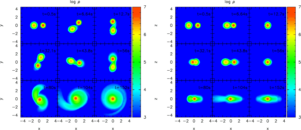 |
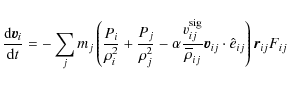
Figure 1:
Temporal evolution of the density for the coalescence of the
|
| Open with DEXTER | |
The equation of state adopted for the white dwarf is the sum of three
components. The ions are treated as an ideal gas but take the Coulomb
corrections into account (Segretain et al. 1994). We have also
incorporated the pressure of photons, which turns out to be important
when the temperature is high and the density is small, just when
nuclear reactions become relevant. Finally the most important
contribution is the pressure of degenerate electrons, which is treated
by integrating the Fermi-Dirac integrals. The nuclear network adopted
here (Benz et al. 1989a) incorporates 14 nuclei: He, C,
O, Ne, Mg, Si, S, Ar, Ca, Ti, Cr, Fe, Ni, and Zn. The reactions
considered are captures of ![]() particles, and the associated back
reactions, the fussion of two C nuclei, and the reaction between C and
O nuclei. All the rates are taken from Rauscher & Thielemann (2000).
The screening factors adopted in this work are those of Itoh
et al. (1979). The nuclear energy release is computed independently of
the dynamical evolution with much shorter time steps, assuming that
the dynamical variables do not change much during these time steps.
Finally, neutrino losses have also been included according to the
formulation of Itoh et al. (1996) for the pair, photo, plasma, and
bremsstrahlung neutrino processes.
particles, and the associated back
reactions, the fussion of two C nuclei, and the reaction between C and
O nuclei. All the rates are taken from Rauscher & Thielemann (2000).
The screening factors adopted in this work are those of Itoh
et al. (1979). The nuclear energy release is computed independently of
the dynamical evolution with much shorter time steps, assuming that
the dynamical variables do not change much during these time steps.
Finally, neutrino losses have also been included according to the
formulation of Itoh et al. (1996) for the pair, photo, plasma, and
bremsstrahlung neutrino processes.
For the integration method, we use a predictor-corrector numerical scheme with variable time steps (Serna 1996), which turns out to be quite accurate. Each particle is followed by individual time steps. With this procedure the energy and angular momentum of the system are conserved with good accuracy. To avoid numerical artifacts, we only use equal-mass SPH particles, as in Yoon et al. (2007). This was not the case for the simulations of Guerrero et al. (2004) in which the masses of the SPH particles were different for each one of the coalescing white dwarfs. To achieve an equilibrium initial configuration, we relaxed each individual model star separately, so the two coalescing white dwarfs are spherically symmetric at the beginning of our simulations, as was the case in all previous simulations of this kind. In all the cases the two white dwarfs are initially in a circular orbit at a greater distance than the corresponding Roche lobe radius of the less massive component. The systems are not synchronized because, at least in the stage previous to the coalescence itself, the time scale for loss of angular momentum due to the emission of gravitational radiation is so small that it remains quite unlikely that there exists any dissipation mechanism able to ensure synchronization (Segretain et al. 1997). This is the same initial configuration adopted by Yoon et al. (2007), Guerrero et al. (2004), and Segretain et al. (1997). However, as already stated, we will study synchronized systems in a forthcoming publication. To this system we add a very small artificial acceleration term that decreases the separation of both components. Once the secondary fills its Roche lobe, this acceleration term is suppressed. This procedure is quite similar to the one adopted in all previous works (Guerrero et al. 2004; Yoon et al. 2007; Segretain et al. 1997). We adopt this instant as our time origin.
The chemical compositions of the coalescing white dwarfs depend on the
mass of each star. White dwarfs with masses lower than
![]() have pure He cores. For white dwarfs with masses within this
value and
have pure He cores. For white dwarfs with masses within this
value and
![]() we adopt the corresponding chemical
composition, namely, carbon and oxygen, with mass fractions
we adopt the corresponding chemical
composition, namely, carbon and oxygen, with mass fractions
![]() and
and
![]() uniformingly distributed throughout the
core. Finally, white dwarfs more massive than
uniformingly distributed throughout the
core. Finally, white dwarfs more massive than
![]() have
ONe cores of the appropriate composition (Ritossa et al. 1996). This
is essential in studying the resulting chemical composition of the
merger, as shown in Sect. 3, and it is a clear improvement over recent
high-resolution simulations (Yoon et al. 2007) in which only a single
system of two carbon-oxygen white dwarfs was studied.
have
ONe cores of the appropriate composition (Ritossa et al. 1996). This
is essential in studying the resulting chemical composition of the
merger, as shown in Sect. 3, and it is a clear improvement over recent
high-resolution simulations (Yoon et al. 2007) in which only a single
system of two carbon-oxygen white dwarfs was studied.
3 Results
Figure 1 shows the temporal evolution of the
logarithm of the density for the coalescence of the
![]() white dwarf binary system. In the left panels the positions
of the SPH particles have been projected onto the equatorial plane and
in the right panels onto the polar plane. Time (in seconds) is shown
in the upper right corner of each panel. As can be seen in the
uppermost left panels, the initial configurations of both white dwarfs
are symmetric. Soon after, the less massive white dwarf fills its
Roche lobe and mass tranfer begins, as can be seen in the top central
panel of this figure. The top right panel of
Fig. 1 shows that, after some time, the matter flowing
out of the secondary hits the surface of the primary white dwarf and
spreads on top of it. We note as well that since the radius of white
dwarfs scales as
white dwarf binary system. In the left panels the positions
of the SPH particles have been projected onto the equatorial plane and
in the right panels onto the polar plane. Time (in seconds) is shown
in the upper right corner of each panel. As can be seen in the
uppermost left panels, the initial configurations of both white dwarfs
are symmetric. Soon after, the less massive white dwarf fills its
Roche lobe and mass tranfer begins, as can be seen in the top central
panel of this figure. The top right panel of
Fig. 1 shows that, after some time, the matter flowing
out of the secondary hits the surface of the primary white dwarf and
spreads on top of it. We note as well that since the radius of white
dwarfs scales as ![]() M-1/3 and since the secondary loses mass
its radius increases and, hence, the mass-loss rate of the secondary
increases, thus leading to a positive feedback of the process. As a
consequence of this positive feedback an accretion arm is formed that
extends from the remnant of the secondary white dwarf (central panels
in Fig. 1) to the surface of the primary white
dwarf. This accretion arm becomes entangled as a consequence of the
orbital motion of the coalescing white dwarfs and adopts a spiral
shape (bottom left panel). Ultimately, the secondary is totally
disrupted and a heavy disk is formed around the primary (bottom
central panel of Fig. 1). The bottom right panel
of Fig. 1 shows that at time t=152 s the disk is
still not well formed and the remnant of a spiral arm still persists.
We followed the evolution of this merger for some more time and we
found that the final configuration has cylindrical symmetry, that most
of the orbits of the SPH particles belonging to the secondary have
been circularized, and that the spiral pattern has totally
disappeared. At the end of the simulations the radial extension of
the disk is
M-1/3 and since the secondary loses mass
its radius increases and, hence, the mass-loss rate of the secondary
increases, thus leading to a positive feedback of the process. As a
consequence of this positive feedback an accretion arm is formed that
extends from the remnant of the secondary white dwarf (central panels
in Fig. 1) to the surface of the primary white
dwarf. This accretion arm becomes entangled as a consequence of the
orbital motion of the coalescing white dwarfs and adopts a spiral
shape (bottom left panel). Ultimately, the secondary is totally
disrupted and a heavy disk is formed around the primary (bottom
central panel of Fig. 1). The bottom right panel
of Fig. 1 shows that at time t=152 s the disk is
still not well formed and the remnant of a spiral arm still persists.
We followed the evolution of this merger for some more time and we
found that the final configuration has cylindrical symmetry, that most
of the orbits of the SPH particles belonging to the secondary have
been circularized, and that the spiral pattern has totally
disappeared. At the end of the simulations the radial extension of
the disk is ![]()
![]() ,
whereas its height is
,
whereas its height is
![]()
![]() .
.
The temporal evolution of the temperature for the merger of a
![]() binary system is shown in Fig. 2. As
can be seen in this figure, the material of the secondary is first
heated by tidal torques. As the secondary begins the disruption
process this material is transferred to the surface of the primary
and, consequently, compressed, and its temperature increases. The
peak temperatures (
binary system is shown in Fig. 2. As
can be seen in this figure, the material of the secondary is first
heated by tidal torques. As the secondary begins the disruption
process this material is transferred to the surface of the primary
and, consequently, compressed, and its temperature increases. The
peak temperatures (
![]() )
achieved during the coalescence are
displayed in Table 1 for each one of the runs presented
in this paper. For the
)
achieved during the coalescence are
displayed in Table 1 for each one of the runs presented
in this paper. For the
![]() simulation, the peak
temperature is
simulation, the peak
temperature is
![]() K, clearly higher
than the carbon ignition temperature
K, clearly higher
than the carbon ignition temperature
![]() K, and
occurs during the first and most violent part of the merger. However,
a strong thermonuclear flash does not develop because, although the
temperature in the region where the material of the secondary first
hits the primary increases very rapidly, degeneracy is rapidly lifted,
leading to an expansion of the material, which, in turn, quenches the
thermonuclear flash. This agrees with the results of Guerrero et al.
(2004) and Yoon et al. (2007). Thus, since these high temperatures
are only attained during a very short time interval, thermonuclear
processing is very mild for this simulation. It is also interesting
to compare the equatorial and polar distribution of temperatures shown
in the central panels of Fig. 2. This comparison
reveals that the heated material is rapidly redistributed on the
surface of the primary, and as a consequence, a hot corona forms
around the primary. The spiral structure previously described can be
more easily appreciated in the bottom right panels of
Fig. 2. In fact, this spiral structure persists for
some more time.
K, and
occurs during the first and most violent part of the merger. However,
a strong thermonuclear flash does not develop because, although the
temperature in the region where the material of the secondary first
hits the primary increases very rapidly, degeneracy is rapidly lifted,
leading to an expansion of the material, which, in turn, quenches the
thermonuclear flash. This agrees with the results of Guerrero et al.
(2004) and Yoon et al. (2007). Thus, since these high temperatures
are only attained during a very short time interval, thermonuclear
processing is very mild for this simulation. It is also interesting
to compare the equatorial and polar distribution of temperatures shown
in the central panels of Fig. 2. This comparison
reveals that the heated material is rapidly redistributed on the
surface of the primary, and as a consequence, a hot corona forms
around the primary. The spiral structure previously described can be
more easily appreciated in the bottom right panels of
Fig. 2. In fact, this spiral structure persists for
some more time.
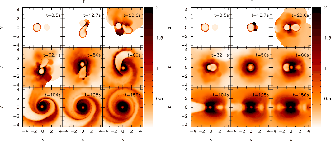 |
Figure 2: Temporal evolution of the temperature (in units of 109 K) for the coalescence of the same binary system shown in Fig. 1. The positions of the particles have been projected onto the xy plane ( left panels) and on the xz plane ( right panels). These figures use the visualization tool SPLASH (Price 2007). (Color figure only available in the electronic version of the article). |
| Open with DEXTER | |
Table 1: Summary of hydrodynamical results.
In all the cases studied here, a self-gravitating structure forms
after a few orbital periods, in agreement with our previous findings
(Guerrero et al. 2004) and with those of Yoon et al. (2007). The time
necessary for its formation depends on the system being studied and
ranges from
![]() s to
s to
![]() s. This
self-gravitating structure consists in all the cases but that in which
two equal-mass white dwarfs are involved in a compact central object,
surrounded by a heavy keplerian disk of variable extension. The case
in which two
s. This
self-gravitating structure consists in all the cases but that in which
two equal-mass white dwarfs are involved in a compact central object,
surrounded by a heavy keplerian disk of variable extension. The case
in which two
![]() white dwarfs are involved the
configuration is rather different. There the symmetry of the systems
avoids the formation of a clear disk structure, instead giving rise to
a rotating elipsoid around the central compact object, surrounded by a
considerably smaller disk. In Table 1 we summarize the
most relevant parameters of all the mergers studied here. Columns
two, three, four, and five list, respectively, the mass of the central
white dwarf obtained after the disruption of the secondary, the mass
of the Keplerian disk, the accreted and the ejected mass. All the
masses are expressed in solar units. In column six we show the peak
temperatures achieved during the coalescence. In column seven we
display the temperature of the hot corona around the central object by
the end of our simulations, whereas in column eight the radius of the
disk is shown. In column nine we list the disk half thickness.
Column
ten displays the duration of the coalescence process and columns
eleven, twelve, and thirteen display the energetics of the process.
In particular we show the thermonuclear energy released during the
coalescence process (
white dwarfs are involved the
configuration is rather different. There the symmetry of the systems
avoids the formation of a clear disk structure, instead giving rise to
a rotating elipsoid around the central compact object, surrounded by a
considerably smaller disk. In Table 1 we summarize the
most relevant parameters of all the mergers studied here. Columns
two, three, four, and five list, respectively, the mass of the central
white dwarf obtained after the disruption of the secondary, the mass
of the Keplerian disk, the accreted and the ejected mass. All the
masses are expressed in solar units. In column six we show the peak
temperatures achieved during the coalescence. In column seven we
display the temperature of the hot corona around the central object by
the end of our simulations, whereas in column eight the radius of the
disk is shown. In column nine we list the disk half thickness.
Column
ten displays the duration of the coalescence process and columns
eleven, twelve, and thirteen display the energetics of the process.
In particular we show the thermonuclear energy released during the
coalescence process (
![]() ), the neutrino energy (
), the neutrino energy (![]() ),
and the energy radiated in the form of gravitational waves (
),
and the energy radiated in the form of gravitational waves (
![]() ). Finally, in column fourteen we list the angular velocities of
the central compact remnants.
). Finally, in column fourteen we list the angular velocities of
the central compact remnants.
As can be seen, for the first two simulations the accreted mass is
approximately the same and the same occurs for the last two
simulations. As already said, the simulation in which two equal-mass
white dwarfs are involved is rather special and in this case we do not
have a disk properly speaking, although a very flattened region with
cylindrical symmetry forms around a central object of ellipsoidal
shape. The mass of this region is ![]()
![]() .
In all five
cases, the mass ejected from the system (those particles which acquire
velocities higher than the escape velocity) is very low
(
.
In all five
cases, the mass ejected from the system (those particles which acquire
velocities higher than the escape velocity) is very low
(![]()
![]() ), and thus the merging process can be considered
as conservative. The maximum temperatures of the coronae increase as
the total mass of the binary system increases. It should be noted
that, for the case of the
), and thus the merging process can be considered
as conservative. The maximum temperatures of the coronae increase as
the total mass of the binary system increases. It should be noted
that, for the case of the
![]() binary system, the
maximum temperature occurs at the center of the merged configuration.
We have found that these temperatures are somewhat lower than those
obtained in our previous simulations (Guerrero et al. 2004). This is
a direct consequence of the improved treatment of the artificial
viscosity and of the enhanced spatial resolution. For instance, we
have found that by using an enhanced resolution and an improved
prescription for the viscosity, the peak temperature obtained in the
simulation in which a 0.6 and
binary system, the
maximum temperature occurs at the center of the merged configuration.
We have found that these temperatures are somewhat lower than those
obtained in our previous simulations (Guerrero et al. 2004). This is
a direct consequence of the improved treatment of the artificial
viscosity and of the enhanced spatial resolution. For instance, we
have found that by using an enhanced resolution and an improved
prescription for the viscosity, the peak temperature obtained in the
simulation in which a 0.6 and
![]() are involved is
are involved is
![]() K - see Table 1. When a
reduced number of SPH particles and the classical expression for the
artificial viscosity are used, this temperature is
K - see Table 1. When a
reduced number of SPH particles and the classical expression for the
artificial viscosity are used, this temperature is
![]() K, whereas the peak temperature turns out to be
K, whereas the peak temperature turns out to be
![]() K when a reduced number of
particles and an improved artificial viscosity are used. It is worth
noting that the radial extension of the disks is roughly the same for
all but one the simulations presented here, and it is considerably
smaller for the case in which two equal-mass white dwarfs are
involved. This is a natural behavior since the central object is
rather massive in this last case. Finally, it is just as interesting
to realize that all the disks are rather thin, being the typical
half-thickness on the order of
K when a reduced number of
particles and an improved artificial viscosity are used. It is worth
noting that the radial extension of the disks is roughly the same for
all but one the simulations presented here, and it is considerably
smaller for the case in which two equal-mass white dwarfs are
involved. This is a natural behavior since the central object is
rather massive in this last case. Finally, it is just as interesting
to realize that all the disks are rather thin, being the typical
half-thickness on the order of ![]()
![]() ,
much smaller
than the typical disk radial extension,
,
much smaller
than the typical disk radial extension, ![]()
![]() .
.
The chemical composition of the disk formed by the disrupted secondary
can be found for all the simulations presented in this paper in
Table 2. In this table we show, for each of the mergers
computed here, the averaged chemical composition (mass fractions) of
the heavily rotationally-supported disk - left section of
Table 2 - and the hot corona - right section - described
previously. For the mergers in which two carbon-oxygen white dwarfs
are involved, the disk is mainly formed by carbon and oxygen and the
nuclear processing is very small (see the peak temperatures shown in
column ten of Table 1). This is not the case for the
simulations in which a lighter He white dwarf is involved. Since in
these cases the Coulomb barrier is considerably smaller, the shocked
material is nuclearly processed and heavy isotopes form. This is more
evident for the case in which a massive He white dwarf of
![]() is disrupted by a massive CO white dwarf of
is disrupted by a massive CO white dwarf of
![]() - third and eight columns in Table 2. In
this case the abundances in the disk and the hot corona are rather
large. Also, the abundances of heavy nuclei in the hot
corona are much larger than those of the disk, indicating that most of
the nuclear reactions occur when the accretion stream hits the surface
of the primary.
- third and eight columns in Table 2. In
this case the abundances in the disk and the hot corona are rather
large. Also, the abundances of heavy nuclei in the hot
corona are much larger than those of the disk, indicating that most of
the nuclear reactions occur when the accretion stream hits the surface
of the primary.
Table 2: Averaged chemical composition (mass fractions) of the heavy rotationally-supported disk and the hot corona obtained by the end of the coalescing process.
Although the disk is primarily made of the He coming from the
disrupted secondary, the abundances of C and O are sizeable; moreover,
the disk is contaminated by heavy metals. This has important
consequences because it is thought that some of the recently
discovered metal-rich DA white dwarfs with dusty disks around them -
also known as DAZd white dwarfs - could be formed by accretion of a
minor planet. The origin of such minor planets still remains a
mystery, since asteroids sufficiently close to the white dwarf would
have not survived the AGB phase (Villaver & Livio 2007). However,
planet formation in these metal-rich disks is expected to be fairly
efficient, thus providing a natural environment where minor planetary
bodies could be formed and, ultimately, tidally disrupted to produce
the observed abundance pattern in these white dwarfs
(García-Berro et al. 2007). Nuclear reactions are also important in the
case in which a regular
![]() carbon-oxygen white dwarf and
a massive oxygen-neon white dwarf of
carbon-oxygen white dwarf and
a massive oxygen-neon white dwarf of
![]() are involved.
In this case the peak temperature achieved during the coalescence is
relatively high
are involved.
In this case the peak temperature achieved during the coalescence is
relatively high
![]() - see
Table 1 - enough to power carbon burning. Consequently, the
chemical abundances of the Keplerian disk and of the hot corona are
largely enhanced in oxygen and neon, which are the main products of
carbon burning. We must add, however, a cautionary remark regarding
the chemical compositions of the mergers studied here. White dwarfs
are characterized in
- see
Table 1 - enough to power carbon burning. Consequently, the
chemical abundances of the Keplerian disk and of the hot corona are
largely enhanced in oxygen and neon, which are the main products of
carbon burning. We must add, however, a cautionary remark regarding
the chemical compositions of the mergers studied here. White dwarfs
are characterized in ![]()
![]() of the cases by a thin hydrogen
atmosphere of
of the cases by a thin hydrogen
atmosphere of ![]()
![]() on top of a helium buffer of
on top of a helium buffer of
![]()
![]() .
In the remaining
.
In the remaining ![]()
![]() of the cases,
the hydrogen atmosphere is absent. Small amounts of helium could
indeed change the nucleosynthetic pattern of the hot corona in all
these cases. Studying this possibility is beyond the scope of this
paper and, thus, the changes in the abundances associated to burning
of the helium buffer and of the atmospheric hydrogen remain to be
explored.
of the cases,
the hydrogen atmosphere is absent. Small amounts of helium could
indeed change the nucleosynthetic pattern of the hot corona in all
these cases. Studying this possibility is beyond the scope of this
paper and, thus, the changes in the abundances associated to burning
of the helium buffer and of the atmospheric hydrogen remain to be
explored.
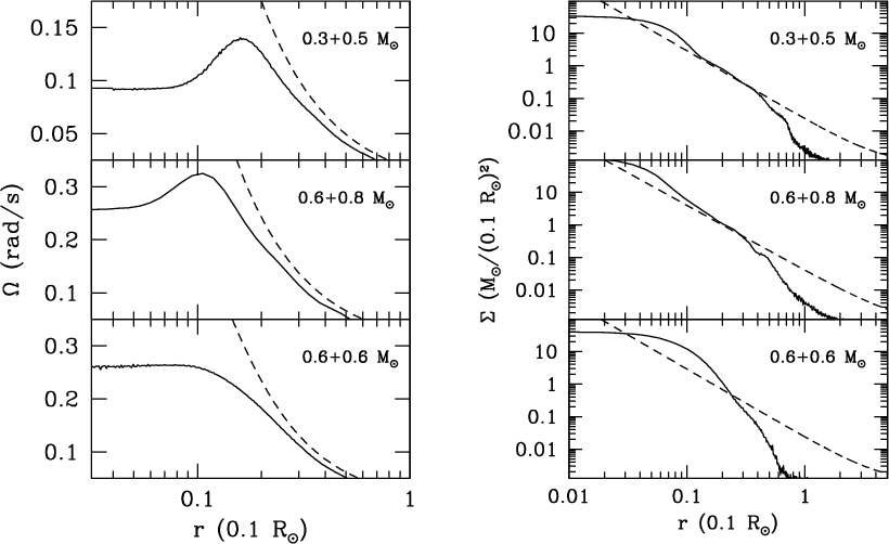 |
Figure 3: Left panels: rotational velocity of the merger products as a function of the radius. For the sake of comparison the Keplerian velocity is also shown as a dashed line. Right panels: surface density profiles compared with the theoretical thin disk model profiles (dashed lines). |
| Open with DEXTER | |
In Fig. 3 we explore the final characteristics of the merged
configuration. We start discussing the left panels of
Fig. 3, which show the rotational velocity of the merger as a
function of the distance to the center of the merged object. Clearly
in all the cases there is a central region that rotates as rigid solid
- see last column of Table 1. This behavior has
already been found in Guerrero et al. (2004) and Yoon et al. (2007)
and is a consequence of the conservation of angular momentum. A
differentially rotating layer is present on top of this region. This
rapidly rotating region is formed by material coming from the
disrupted secondary, which has been accumulated on top of the primary
and thus carries the original angular moment of the secondary.
Finally, a rotationally-supported disk is found for a large enough
radius. The exact location where the disk begins can be easily found
by looking at the left panels of Fig. 3, where the
Keplerian velocity is also shown. The change in the slope of the
profile of the rotational velocity clearly marks the outer edge of the
compact inner object and the beginning of the disk. All the disks
extend up to some solar radii - see column eight in
Table 1. The stratification of surface densities of these
disks can be seen in the left panels of Fig. 3, where we
have plotted the surface density as a function of the distance. For
the sake of comparison, the theoretical surface density of a thin disk
analytical model (Livio et al. 2005) is also shown. Within
this model the surface density of the disk should be of the form
![]() .
We used
.
We used ![]() to produce the
dashed lines in the right panels of Fig. 3, very close to
the value adopted by Livio et al. (2005),
to produce the
dashed lines in the right panels of Fig. 3, very close to
the value adopted by Livio et al. (2005), ![]() .
As can be
seen in this figure for the first two fiducial mergers studied here
there is a region where the analytical model and the numerical results
are in good agreement. However, at long enough distances, the SPH
density profile falls off more rapidly than that of the theoretical
model. The agreement is poor in the case of the merger of two
equal-mass
.
As can be
seen in this figure for the first two fiducial mergers studied here
there is a region where the analytical model and the numerical results
are in good agreement. However, at long enough distances, the SPH
density profile falls off more rapidly than that of the theoretical
model. The agreement is poor in the case of the merger of two
equal-mass
![]() white dwarfs. In this case, the symmetry
of the system avoids the formation of a clear disk structure, instead
giving rise to a rotating ellipsoid around the central compact object.
Moreover, it can be shown that the angular momentum of the disk can be
expressed in terms of the disk radius
white dwarfs. In this case, the symmetry
of the system avoids the formation of a clear disk structure, instead
giving rise to a rotating ellipsoid around the central compact object.
Moreover, it can be shown that the angular momentum of the disk can be
expressed in terms of the disk radius
![]() and the disk mass
and the disk mass
![]() as
as
![]() ,
where
,
where
![]() .
The
theoretical angular moments obtained using this equation agree very
well with the results of our SPH simulations.
.
The
theoretical angular moments obtained using this equation agree very
well with the results of our SPH simulations.
In Fig. 4 we show the temperature profiles at the end of
the simulations for some of the mergers studied here. We averaged the
temperatures of those particles close to the orbital plane. The
average was done using cylindrical shells, and the size of these
shells was chosen in such a way that each of them contains a
significative number of particles. As can be seen, for the
![]() and the
and the
![]() systems, the region of
maximum temperatures occurs off-center, at the edge of the original
primary, in the region of accreted and shocked material, whereas for
the merger in which two equal-mass
systems, the region of
maximum temperatures occurs off-center, at the edge of the original
primary, in the region of accreted and shocked material, whereas for
the merger in which two equal-mass
![]() white dwarfs
coalesce the maximum temperature occurs at the center of the merged
object, as should be expected. These maximum temperatures are listed
in the seventh column of Table 1. In fact, the
temperature profiles shown in this figure clearly show that the cores
of the primaries in the first two simulations almost remain intact
and, hence, are rather cold. These cores, in turn, are surrounded by
a hot envelope that corresponds to the shocked material coming from
the disrupted secondary. Nuclear reactions are responsible for the
observed heating of the accreted matter, initially triggered in the
shocked regions.
white dwarfs
coalesce the maximum temperature occurs at the center of the merged
object, as should be expected. These maximum temperatures are listed
in the seventh column of Table 1. In fact, the
temperature profiles shown in this figure clearly show that the cores
of the primaries in the first two simulations almost remain intact
and, hence, are rather cold. These cores, in turn, are surrounded by
a hot envelope that corresponds to the shocked material coming from
the disrupted secondary. Nuclear reactions are responsible for the
observed heating of the accreted matter, initially triggered in the
shocked regions.
The case in which two
![]() white dwarfs coalesce is
somewhat different. In this case there is no hot envelope around a
central object - although a local maximum of temperatures can indeed
be appreciated at the edge of the rapidly spinning central object, as
shown in the bottom panel of Fig. 4 - and, instead, the
central region of the compact object is formed by the cores of the
merging white dwarfs. Most of the temperature increase in this case
stems from viscous heating since nuclear reactions are negligible
because the increase in temperature of the shocked material is not
enough to ignite carbon. In all these cases, a sizeable dispersion of
temperatures in the outermost regions is apparent. This dispersion is
due in part to this region containing some of the particles that were
ejected during the first and most violent phases of the merging
process.
white dwarfs coalesce is
somewhat different. In this case there is no hot envelope around a
central object - although a local maximum of temperatures can indeed
be appreciated at the edge of the rapidly spinning central object, as
shown in the bottom panel of Fig. 4 - and, instead, the
central region of the compact object is formed by the cores of the
merging white dwarfs. Most of the temperature increase in this case
stems from viscous heating since nuclear reactions are negligible
because the increase in temperature of the shocked material is not
enough to ignite carbon. In all these cases, a sizeable dispersion of
temperatures in the outermost regions is apparent. This dispersion is
due in part to this region containing some of the particles that were
ejected during the first and most violent phases of the merging
process.
In summary, we find that the qualitative behavior of all the mergers studied here is similar. In particular the less massive component of the binary system is disrupted in a few orbital periods. Additionally, we find that nuclear reactions are only important in the cases in which the secondary is a He white dwarf or in the case in which the primary (the accretor) is an ONe white dwarf. The total ejected mass is very small in all these cases. Finally, the overall final configuration is very similar in all them but when two equal-mass white dwarfs coalesce.
4 Comparison with previous works
As previously discussed, all the mergers studied here coalesce on a
dynamical time scale, regardless of its mass ratio. In agreement with
previous calculations, the central regions of the remnant rotate as a
rigid body. On top of this rapidly spinning core, a hot corona forms
and, on top of that, a heavy Keplerian disk. The question is now how
the main characteristics of the merged configuration compare with
those obtained in previous works? Yoon et al. (2007) computed the
coalescence of a single
![]() binary system and the
comparison is not straightforward, but our
binary system and the
comparison is not straightforward, but our
![]() run is
similar. The first thing to be noted is that the duration of the
merger is very similar in both cases. We obtained a duration of 164 s
and Yoon et al. (2007) obtain
run is
similar. The first thing to be noted is that the duration of the
merger is very similar in both cases. We obtained a duration of 164 s
and Yoon et al. (2007) obtain ![]() 150 s. The central density of the
rapidly spinning core is in both cases
150 s. The central density of the
rapidly spinning core is in both cases
![]() g/cm3. The
temperature of the core is
g/cm3. The
temperature of the core is
![]() ,
whereas Yoon et al. (2007)
obtain
,
whereas Yoon et al. (2007)
obtain
![]() ,
but this is due to our choice of the initial
temperature of the coalescing white dwarfs, for which we adopted
T=107 K. The temperatures of the hot coronae are remarkably
similar in both cases,
,
but this is due to our choice of the initial
temperature of the coalescing white dwarfs, for which we adopted
T=107 K. The temperatures of the hot coronae are remarkably
similar in both cases,
![]() and 8.6, respectively. The
peak temperatures attained during the merger are also very similar -
and 8.6, respectively. The
peak temperatures attained during the merger are also very similar -
![]() K and
K and
![]() K, respectively. However, the
temperature of the hot coronae is considerably lower in their case
K, respectively. However, the
temperature of the hot coronae is considerably lower in their case
![]() K. This value has to be compared
with that shown in Table 1,
K. This value has to be compared
with that shown in Table 1,
![]() K. However, it should be taken into account that Yoon
et al. (2007) followed the evolution of the merger for much longer times.
The sizes of the resulting disk are also very similar. Yoon et al.
(2007) obtained
K. However, it should be taken into account that Yoon
et al. (2007) followed the evolution of the merger for much longer times.
The sizes of the resulting disk are also very similar. Yoon et al.
(2007) obtained
![]() cm, whereas we obtain
cm, whereas we obtain
![]() cm. Moreover, despite of the very different approaches for the
artificial viscosities adopted in the work of Yoon et al. (2007) and
in the present work, the rotational velocities of the central spinning
object are very close, 0.21 s-1 in the case of Yoon et al. (2007), whereas we obtain 0.26 s-1. However, we find that
the rotational velocities of the hot coronae are somewhat
different. In particular, Yoon et al. (2007) obtained
cm. Moreover, despite of the very different approaches for the
artificial viscosities adopted in the work of Yoon et al. (2007) and
in the present work, the rotational velocities of the central spinning
object are very close, 0.21 s-1 in the case of Yoon et al. (2007), whereas we obtain 0.26 s-1. However, we find that
the rotational velocities of the hot coronae are somewhat
different. In particular, Yoon et al. (2007) obtained
![]() s-1, while we obtain 0.33 s-1. This could stem from
the different treatment of the artificial viscosity and to the
different masses of the coalescing white dwarfs.
s-1, while we obtain 0.33 s-1. This could stem from
the different treatment of the artificial viscosity and to the
different masses of the coalescing white dwarfs.
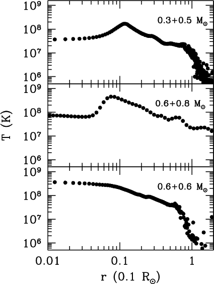 |
Figure 4: Radially averaged temperature profiles as a function of radius. |
| Open with DEXTER | |
The comparison with the results of Guerrero et al. (2004) also yields
interesting results. For instance, the angular velocity of the central
compact object of the
![]() merger in the calculations
of Guerrero et al. (2004) is 0.33 s-1, somewhat larger than that
obtained here. Consequently, the central density obtained in the
simulations of Guerrero et al. (2004) is lower (
merger in the calculations
of Guerrero et al. (2004) is 0.33 s-1, somewhat larger than that
obtained here. Consequently, the central density obtained in the
simulations of Guerrero et al. (2004) is lower (
![]() g/cm3), because of our improved treatment of the artificial
viscosity, which considerably reduces the excess of shear and, thus,
translates into weaker centrifugal forces. Also, the location of the
hot corona is different in the case of the simulations presented here.
Specifically, the hot corona is located at
g/cm3), because of our improved treatment of the artificial
viscosity, which considerably reduces the excess of shear and, thus,
translates into weaker centrifugal forces. Also, the location of the
hot corona is different in the case of the simulations presented here.
Specifically, the hot corona is located at
![]() in the
simulations discussed here, whereas in the case of Guerrero et al. (2004) it was located at
in the
simulations discussed here, whereas in the case of Guerrero et al. (2004) it was located at
![]() .
Also, the temperature
of the central object is smaller in our case (
.
Also, the temperature
of the central object is smaller in our case (
![]() K) than in the case of Guerrero et al. (2004) for which a central
temperature of
K) than in the case of Guerrero et al. (2004) for which a central
temperature of
![]() K was obtained, even though the
initial temperatures of the coalescing white dwarfs were the same in
both cases (107 K). Hence, our improved treatment of the artificial
viscosity results in a smaller overheating and in smaller shear.
K was obtained, even though the
initial temperatures of the coalescing white dwarfs were the same in
both cases (107 K). Hence, our improved treatment of the artificial
viscosity results in a smaller overheating and in smaller shear.
5 Discussion
5.1 Comparison with theory
To obtain a better understanding of the coalescence process and to
compare our results with those theoretically expected, we numerically
solved the equations of the evolution of the binary system during the
mass transfer phase. The evolution of a binary system during this
phase is determined by three basic physical processes, namely,
gravitational wave emission, tidal torques and mass transfer. There
is a wealth of literature dealing with this problem. We adopt as our
starting point the analysis of Marsh et al. (2004) and the more recent
formulation of Gokhale et al. (2007). Within this approach the
evolution of the orbital separation a is given by
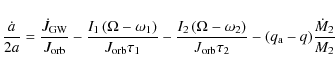
where M1 and M2 are, respectively, the masses of the accretor and of the donor,
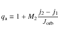 |
(5) |
with j1 the specific angular momentum of the matter arriving to the accretor and j2 the angular momentum of the matter leaving the donor. In the calculations presented here, we have adopted for j1 the expression for disk fed accretion:
 |
(6) |
whereas for j2 we have
 |
(7) |
The first term in Eq. (4) corresponds to the change in the orbital separation due to gravitational losses. Because of the short duration of the coalescing process, its contribution can be neglected. The second and third term describe the tidal couplings. Finally, the last term in Eq. (4) corresponds to the advected angular momentum.
The evolution of the Roche lobe radius ![]() is given by
is given by
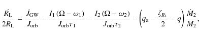
where
An expression for the mass-transfer rate is needed to solve the
previous equations. The mass-transfer rate is essentially determined
by the Roche lobe overfill factor, which is defined as
![]() .
For the Roche lobe radius we adopt the expression
of Eggleton (1983). In the case of a
.
For the Roche lobe radius we adopt the expression
of Eggleton (1983). In the case of a
![]() donor white
dwarf a polytropic equation of state with n=3/2 can be adopted and,
thus, we have (Paczynski & Sienkiewicz 1972):
donor white
dwarf a polytropic equation of state with n=3/2 can be adopted and,
thus, we have (Paczynski & Sienkiewicz 1972):
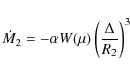
with
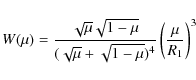 |
(10) |
where
 |
|||
 |
(11) |
where, again, the normalization factors
can be integrated. In doing so it has to be taken into account the logical limitations of the theoretical approach. In particular, the SPH results show that mass transfer is not perfectly conservative, although this assumption is fairly good - see Table 1. Moreover, stars are not point-like masses and, more important, we did not adopt an equilibrium mass-radius relationship in our analysis. These assumptions may produce marked differences between the SPH and the theoretical results. Perhaps the most critical assumption in determining the evolution of the system is assuming that an equilibrium mass-radius relation holds for both members of the binary system. In fact, at the beginning of the mass-transfer episode, stars are not in equilibrium. Consequently, we adopted a different approach. In particular, when integrating Eqs. (12) we have computed for each time step the actual moment of inertia of each star. In particular, in the case of the primary white dwarf for each computed model, we looked for location of the region with maximum temperature (see Fig. 2). We then computed the mass interior to this shell and the corresponding moment of inertia. For the donor white dwarf we looked for the region that still had an approximate spherical symmetry (see Fig. 1) and we followed the same procedure as adopted for the accretor.
 |
Figure 5:
A comparison of the SPH values for the orbital distance a and for the spin angular moments of the donor and the
accretor stars for the
|
| Open with DEXTER | |
In Fig. 5 we compare the theoretical results - shown
as a dashed line - and the SPH results - shown as dots - for the
time evolution of the orbital separation and of the spin angular
moment of the accretor (J1) and donor stars (J2). The three
adjustable parameters adopted in the theoretical calculations are,
respectively,
![]() ,
,
![]() yr and
yr and
![]() yr. As
can be seen, the agreement is excellent during the first phases of the
merger. However, we can only compare the SPH results with the
theoretical expectations, while the secondary still partially
preserves its initial shape. This is why we only show a reduced time
interval in Fig. 5, corresponding to the first five
panels in Figs. 1 and 2. For times
longer than
yr. As
can be seen, the agreement is excellent during the first phases of the
merger. However, we can only compare the SPH results with the
theoretical expectations, while the secondary still partially
preserves its initial shape. This is why we only show a reduced time
interval in Fig. 5, corresponding to the first five
panels in Figs. 1 and 2. For times
longer than ![]() 70 s, the secondary rapidly dissolves, hence, the
approach followed here is no longer valid. It is worth realizing that
70 s, the secondary rapidly dissolves, hence, the
approach followed here is no longer valid. It is worth realizing that
![]() .
This means that the synchronization timescale
of the primary is much larger than that of the secondary.
Accordingly, during this phase of the mass-transfer episode, the donor
rapidly synchronizes, whereas the primary does not. Consequently,
orbital angular moment is transferred from the orbit to the donor on a
short timescale, thus reducing the orbital separation. This, in turn,
increases the mass-transfer rate and the final result is that the
secondary is rapidly disrupted. Since the total angular momentum is
conserved, the material transferred to the primary must rotate
rapidly, thus producing the characteristic rotational profiles shown
in the left panels of Fig. 3. In summary, the results of
the hydrodynamic calculations can be accurately reproduced by a simple
model once all the weaknesses of the theoretical approach are
correctly taken into account.
.
This means that the synchronization timescale
of the primary is much larger than that of the secondary.
Accordingly, during this phase of the mass-transfer episode, the donor
rapidly synchronizes, whereas the primary does not. Consequently,
orbital angular moment is transferred from the orbit to the donor on a
short timescale, thus reducing the orbital separation. This, in turn,
increases the mass-transfer rate and the final result is that the
secondary is rapidly disrupted. Since the total angular momentum is
conserved, the material transferred to the primary must rotate
rapidly, thus producing the characteristic rotational profiles shown
in the left panels of Fig. 3. In summary, the results of
the hydrodynamic calculations can be accurately reproduced by a simple
model once all the weaknesses of the theoretical approach are
correctly taken into account.
5.2 Gravitational wave radiation
Gravitational wave radiation from Galactic close white dwarf binary
systems is expected to be the dominant contribution to the background
noise in the low frequency region, which ranges from ![]() 10-3 up
to
10-3 up
to ![]() 10-2 Hz (Bender et al. 1998). Moreover, since a
sizeable amount of mass is transferred from the donor star to the
primary at considerable speeds during the merging process, the
gravitational wave signal is expected to be detectable by LISA
(Guerrero et al. 2004; Lorén-Aguilar et al. 2005). It is thus
important to characterize which would be the gravitational wave
emission of the white dwarf mergers studied here and to assess the
feasibility of dectecting them.
10-2 Hz (Bender et al. 1998). Moreover, since a
sizeable amount of mass is transferred from the donor star to the
primary at considerable speeds during the merging process, the
gravitational wave signal is expected to be detectable by LISA
(Guerrero et al. 2004; Lorén-Aguilar et al. 2005). It is thus
important to characterize which would be the gravitational wave
emission of the white dwarf mergers studied here and to assess the
feasibility of dectecting them.
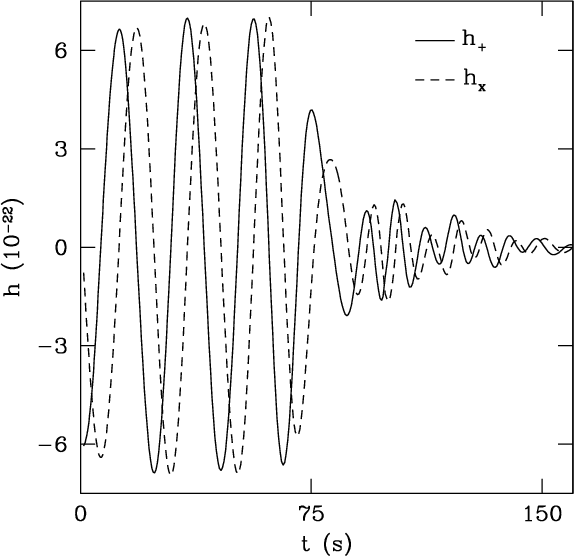 |
Figure 6:
Gravitational wave emission from the merger of a
|
| Open with DEXTER | |
To compute the gravitational wave pattern, we proceed as in
Lorén-Aguilar et al. (2005). In particular, we use the weak-field
quadrupole approximation (Misner et al. 1973):
where t-R=t-d/c is the retarded time, d the distance to the observer, and
To calculate the quadrupole moment of the mass distribution using SPH particles, Eq. (14) must be discretized according to the following expression
where
is the transverse-traceless projection operator onto the plane orthogonal to the outgoing wave direction,
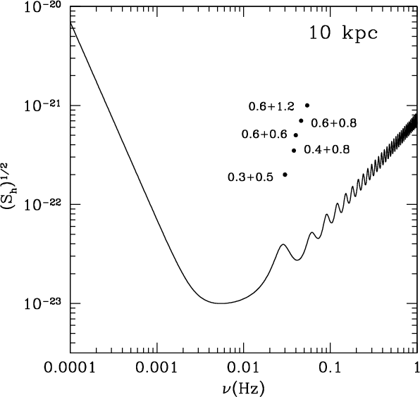 |
Figure 7:
A comparison of the signal produced by the close white dwarf
binary systems studied here when a distance of 10 kpc is
adopted, with the spectral distribution of noise of LISA. The
spectral distribution of noise of LISA is for a one-year
integration period. We have adopted a signal-to-noise ratio
|
| Open with DEXTER | |
Using this prescription, the corresponding strains for the
![]() ,
which is a representative case, are shown in
Fig. 6. As can be seen, the gravitational waveforms rapidly vanish
in a couple of orbital periods and the gravitational wave emission
during the coalescence phase does not have a noticeably strong
peak. Hence, the gravitational wave emission is dominated by the
chirping phase, in agreement with the findings of Lorén-Aguilar
et al. (2005). Moreover, the gravitational waveforms obtained here are
very similar to those computed by Lorén-Aguilar et al. (2005) and,
thus, do not depend appreciably on the number of particles used to
calculate them. This is because most of the emission of gravitational
waves comes from the regions in which the SPH particles change
appreciably their velocities, and these regions were well resolved in
both sets of simulations. Higher order terms of gravitational wave
emission could be included in calculating the strains. These terms
include the current-quadrupole and the mass octupole. It has been
shown (Schutz & Ricci 2001) that, for the first of these to be
relevant, an oscillating angular momentum distribution with a dipole
moment along the angular momentum axis is needed. Consequently, in
our calculations only the mass octupole should be considered in the
best of the cases. Within this approximation, a term close to
,
which is a representative case, are shown in
Fig. 6. As can be seen, the gravitational waveforms rapidly vanish
in a couple of orbital periods and the gravitational wave emission
during the coalescence phase does not have a noticeably strong
peak. Hence, the gravitational wave emission is dominated by the
chirping phase, in agreement with the findings of Lorén-Aguilar
et al. (2005). Moreover, the gravitational waveforms obtained here are
very similar to those computed by Lorén-Aguilar et al. (2005) and,
thus, do not depend appreciably on the number of particles used to
calculate them. This is because most of the emission of gravitational
waves comes from the regions in which the SPH particles change
appreciably their velocities, and these regions were well resolved in
both sets of simulations. Higher order terms of gravitational wave
emission could be included in calculating the strains. These terms
include the current-quadrupole and the mass octupole. It has been
shown (Schutz & Ricci 2001) that, for the first of these to be
relevant, an oscillating angular momentum distribution with a dipole
moment along the angular momentum axis is needed. Consequently, in
our calculations only the mass octupole should be considered in the
best of the cases. Within this approximation, a term close to
![]() would be added to the derived strains. We performed
a post-processing of our simulations and we find that the octupole
emission is
would be added to the derived strains. We performed
a post-processing of our simulations and we find that the octupole
emission is
![]() ,
just above the numerical noise (
,
just above the numerical noise (
![]() ), but in either case totally negligible. Since the
gravitational wave signal is dominated by that of the inspiralling
phase, to assess the feasibility of detecting it using gravitational
wave detectors, we assumed that the orbital separation of the binary
system is that of the last stable orbit. Furthermore, we also assumed
that the integration time of LISA will be one year. It is then
straightforward to demonstrate that, during this time interval, the
variation in the orbital separation is negligible. With these
assumptions the double white-dwarf binary system basically radiates a
monochromatic wave, and it is easy to assess the feasibility of
detecting the signal produced by the coalescence of close binary white
dwarf systems. This is done in Fig. 7 where we show the
strength of the resulting signals and compare them with the spectral
distribution of noise of LISA, when a distance of 10 kpc is adopted.
As can be seen in this figure, all the systems are well inside the
detectability region, hence, LISA should be able to distinguish them
from Galactic. However, the typical rate of white dwarf mergers is
rather small,
), but in either case totally negligible. Since the
gravitational wave signal is dominated by that of the inspiralling
phase, to assess the feasibility of detecting it using gravitational
wave detectors, we assumed that the orbital separation of the binary
system is that of the last stable orbit. Furthermore, we also assumed
that the integration time of LISA will be one year. It is then
straightforward to demonstrate that, during this time interval, the
variation in the orbital separation is negligible. With these
assumptions the double white-dwarf binary system basically radiates a
monochromatic wave, and it is easy to assess the feasibility of
detecting the signal produced by the coalescence of close binary white
dwarf systems. This is done in Fig. 7 where we show the
strength of the resulting signals and compare them with the spectral
distribution of noise of LISA, when a distance of 10 kpc is adopted.
As can be seen in this figure, all the systems are well inside the
detectability region, hence, LISA should be able to distinguish them
from Galactic. However, the typical rate of white dwarf mergers is
rather small, ![]()
![]() yr-1 (Nelemans 2003);
consequently, although there is an uncertainty of a factor of 5 in the
rate of white dwarf mergers, the expected detection rate is small as
well.
yr-1 (Nelemans 2003);
consequently, although there is an uncertainty of a factor of 5 in the
rate of white dwarf mergers, the expected detection rate is small as
well.
5.3 Fallback luminosities
Another potential observational signature of the mergers studied here is the emission of high-energy photons from the fallback material in the aftermath of the coalescence itself. We have already shown that, as a result of the merger of two white dwarfs of different masses, most of the SPH particles of the disrupted secondary form a Keplerian disk. These SPH particles have circularized orbits. However, as it occurs in the coalescence of double neutron stars, some material of the secondary is also found to be in highly eccentric orbits. After some time, this material will most likely interact with the recently formed disk. As discussed in Rosswog (2007), the timescale for this is not set by viscous dissipation but, instead, by the distribution of eccentrities. We followed the model proposed by Rosswog (2007) closely and calculated the accretion luminosity obtained from the interaction of the stellar material with high eccentricities with the newly formed disk by assuming that the kinetic energy of these particles is dissipated within the radius of the debris disk.
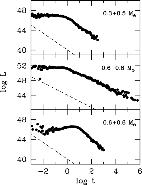 |
Figure 8: Fallback accretion luminosity for our three fiducial double white dwarf mergers. The units of time are seconds, whereas those of luminosities are erg/s. A straight line with slope 5/3 is shown for the sake of comparison. |
| Open with DEXTER | |
In Fig. 8 we have plotted the accretion luminosities as a
function of time for our three fiducial cases. We emphasize that these
luminosities were computed assuming that the highly eccentric
particles lose all their kinetic energy when interacting with the
disk, for which we adopt the radius obtained by the end of our SPH
simulations, which are those shown in Table 1.
Moreover, only a fraction of this energy will be released in the form
of high-energy photons. Thus, the results shown in Fig. 8
can be regarded as an upper limit for the actual luminosity of
high-energy photons. Although the luminosities are lower than those
typically obtained for the merger of double neutron stars - which
are typically ![]() 1052 erg/s - white-dwarf mergers predict a
very similar time dependence (
1052 erg/s - white-dwarf mergers predict a
very similar time dependence (![]() t5/3).
t5/3).
This is an important result because it shows that observations of high-energy photons can help in detecting the gravitational wave signal radiated by these systems. In fact, the detection of the gravitational waves arising from the merger of white dwarfs is a tough task because, as previously explained, the signal is dominated by the inspiralling phase and the waveforms do not have a prominent peak before the ringdown phase. Thus a combined strategy in which optical, UV, X-ray, and gravitational wave detectors are used could be very useful.
5.4 Long-term evolution
We have already shown that non-explosive nuclear burning takes place
during the merging phase. However, this does not necessarily mean that
such an explosion could not take place due to mass accretion from the
disk at late times. If mass acccretion occurs at rates less than
![]() ,
then central carbon ignition is
possible and a type Ia supernova (SNIa) is the most probable outcome.
On the other hand, if the accretion rates are higher than this value,
then off-center carbon ignition is the most probable outcome, giving
rise to an inward propagating burning flame and an ONe white dwarf is
likely to be formed (Nomoto & Iben 1986; García-Berro & Iben
1994; Ritossa et al. 1999) which might eventually form a neutron star
by accretion-induced collapse (Saio & Nomoto 1985; Woosley & Weaver
1986; Gutiérrez et al. 1996, 2005). However, once the disk has been
formed, angular momentum viscous transfer is relevant and the
hydrodynamical timescale of the disk becomes very large.
Consequently, the subsequent evolution of the disk cannot be followed
using an SPH code. However, some estimates of the accretion rate can
still be done by considering the typical viscous transport timescales.
,
then central carbon ignition is
possible and a type Ia supernova (SNIa) is the most probable outcome.
On the other hand, if the accretion rates are higher than this value,
then off-center carbon ignition is the most probable outcome, giving
rise to an inward propagating burning flame and an ONe white dwarf is
likely to be formed (Nomoto & Iben 1986; García-Berro & Iben
1994; Ritossa et al. 1999) which might eventually form a neutron star
by accretion-induced collapse (Saio & Nomoto 1985; Woosley & Weaver
1986; Gutiérrez et al. 1996, 2005). However, once the disk has been
formed, angular momentum viscous transfer is relevant and the
hydrodynamical timescale of the disk becomes very large.
Consequently, the subsequent evolution of the disk cannot be followed
using an SPH code. However, some estimates of the accretion rate can
still be done by considering the typical viscous transport timescales.
The typical viscous transport timescale is (Mochkovitch & Livio
1989,
1990)
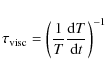
where T is the rotational kinetic energy and
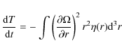 |
(18) |
is its rate of change. In this expression
 |
(19) |
where M* and R* are the mass and radius of the central object. If, instead, the disk is turbulent the classical approximation of Shakura & Sunyaev (1973) is valid. Within this approximation the viscous timescale is given by
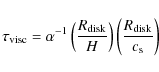 |
(20) |
where

In order to check that the disk is turbulent we have computed the Richardson number
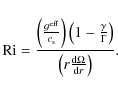 |
(22) |
In this expression
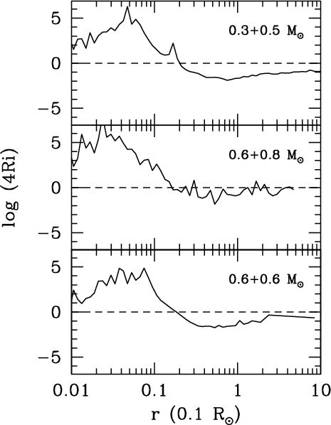 |
Figure 9: Richardson number as a function of the distance. When Ri > 1/4, the disk is turbulent. The horizontal dashed line corresponds to Ri = 1/4. |
| Open with DEXTER | |
Table 3:
Typical viscous timescales (in years), dissipated kinetic
energies (in erg/s), and accretion rates (in
![]() yr-1) when the laminar or the turbulent viscosity are
used.
yr-1) when the laminar or the turbulent viscosity are
used.
Yoon et al. (2007) have systematically explored the conditions for
avoiding off-center carbon ignition in the merged configurations
resulting from the coalescence of two CO white dwarfs. They computed
the evolution of the central remnant of the coalescence of a
![]() binary white dwarf, adopting a realistic initial
model, which includes the differentially rotating primary, the hot
envelope we also find in our simulations and the centrifugally
supported accretion disk. Our final configurations closely resemble
those found by these authors and, consequently, the same conclusions
obtained in this paper hold. In particular, since in our models the
maximum temperature of the hot envelope is lower than the carbon
ignition temperature and the mass-accretion rate from the Keplerian
disk is possibly smaller than the critical one (
binary white dwarf, adopting a realistic initial
model, which includes the differentially rotating primary, the hot
envelope we also find in our simulations and the centrifugally
supported accretion disk. Our final configurations closely resemble
those found by these authors and, consequently, the same conclusions
obtained in this paper hold. In particular, since in our models the
maximum temperature of the hot envelope is lower than the carbon
ignition temperature and the mass-accretion rate from the Keplerian
disk is possibly smaller than the critical one (
![]() ), it is probable that at
least some of the merged configurations with a total mass exceeding
Chandrasekhar's mass may be considered good candidates for Type Ia
supernovae progenitors.
), it is probable that at
least some of the merged configurations with a total mass exceeding
Chandrasekhar's mass may be considered good candidates for Type Ia
supernovae progenitors.
6 Conclusions
We have performed several high-resolution smoothed particle
hydrodynamics simulations of coalescing white dwarfs for a broad range
of masses and chemical compositions of the coalescing white dwarfs,
which includes He, CO, and ONe white dwarfs. Such a parametric study
using a large number of particles (
![]() SPH particles) had
never been done before. Previous works on the subject used a
considerably smaller number - by a factor of 10 - of SPH particles
(Guerrero et al. 2004), or did not explore the full range of masses
and chemical compositions of interest (Yoon et al. 2007) - only one
merger was computed, that of a
SPH particles) had
never been done before. Previous works on the subject used a
considerably smaller number - by a factor of 10 - of SPH particles
(Guerrero et al. 2004), or did not explore the full range of masses
and chemical compositions of interest (Yoon et al. 2007) - only one
merger was computed, that of a
![]() double white
dwarf. In addition, we included a refined treatment of the artificial
viscosity. In particular, we used an artificial viscosity formulation
that is oriented on Riemann-solvers (Monaghan 1997), together with an
additional switch to suppress the excess of viscosity (Balsara 1995).
With this treatment the dissipative terms are only applied in those
regions of the fluid in which they are really needed to resolve a
shock. This refined treatment of the artificial viscosity overcomes
some of the problems found in our previous simulations (Guerrero
et al. 2004).
double white
dwarf. In addition, we included a refined treatment of the artificial
viscosity. In particular, we used an artificial viscosity formulation
that is oriented on Riemann-solvers (Monaghan 1997), together with an
additional switch to suppress the excess of viscosity (Balsara 1995).
With this treatment the dissipative terms are only applied in those
regions of the fluid in which they are really needed to resolve a
shock. This refined treatment of the artificial viscosity overcomes
some of the problems found in our previous simulations (Guerrero
et al. 2004).
In all cases, the merged configuration consists of a compact central
object surrounded by a hot corona with spheroidal shape and a
self-gravitating Keplerian disk around it. For those cases in which
two white dwarfs of different masses are involved, the resulting disk
can be considered as a thin disk, whereas for the
![]() case, we found that the resulting final configuration resembles a
rotating ellipsoid around the central object with a much more modest
disk. The peak temperatures attained during the merging process are
lower than those found by Guerrero et al. (2004) and in line with that
found by Yoon et al. (2007) for the case of a
case, we found that the resulting final configuration resembles a
rotating ellipsoid around the central object with a much more modest
disk. The peak temperatures attained during the merging process are
lower than those found by Guerrero et al. (2004) and in line with that
found by Yoon et al. (2007) for the case of a
![]() merger. We also confirm the results obtained in previous works
(Guerrero et al. 2004: Lorén-Aguilar et al.
2005; Yoon et al. 2007) and find that, only when one of the merging white dwarfs is a He
white dwarf, nuclear reactions are relevant. However, none of the
cases studied here show any explosive behavior during the merging
phase. Furthermore, no essential differences are found when the
chemical abundances obtained here using an enhanced spatial resolution
and a refined prescription for the artificial viscosity and those
obtained in previous works (García-Berro et al.
2007) are
compared. The chemical composition of the disks formed by the
coalescence of a He white dwarf with CO white dwarfs shows an
enrichment in heavy elements like Ca, Mg, S, Si, and Fe and constitute
a natural environment where planets and asteroids can be formed. This
could explain the anomalous abundances of metals found in several
hydrogen-rich white dwarfs with dusty disks around them and that have
been attributed to the impact of asteroids (Jura 2003), since it is
quite unlikely that such asteroids could survive the red giant phase.
merger. We also confirm the results obtained in previous works
(Guerrero et al. 2004: Lorén-Aguilar et al.
2005; Yoon et al. 2007) and find that, only when one of the merging white dwarfs is a He
white dwarf, nuclear reactions are relevant. However, none of the
cases studied here show any explosive behavior during the merging
phase. Furthermore, no essential differences are found when the
chemical abundances obtained here using an enhanced spatial resolution
and a refined prescription for the artificial viscosity and those
obtained in previous works (García-Berro et al.
2007) are
compared. The chemical composition of the disks formed by the
coalescence of a He white dwarf with CO white dwarfs shows an
enrichment in heavy elements like Ca, Mg, S, Si, and Fe and constitute
a natural environment where planets and asteroids can be formed. This
could explain the anomalous abundances of metals found in several
hydrogen-rich white dwarfs with dusty disks around them and that have
been attributed to the impact of asteroids (Jura 2003), since it is
quite unlikely that such asteroids could survive the red giant phase.
We also compared the results of our hydrodynamical calculations with the theoretical expectations and found a satisfactory agreement when the synchronization timescale of the disrupted secondary is much shorter than that of the primary. In this case the rate of change of the orbital distance and the corresponding spins of both the donor star and of the accretor are reproduced with a high degree of accuracy. We have shown as well that the emission of gravitational waves from these kind of systems is strong enough to be obervable by LISA and that the corresponding waveforms do not depend much on the resolution employed in the hydrodynamical calculations and, thus, that these waveforms are robust.
We also computed the possible emission of high-energy photons produced
in the aftermath of the merger. This high-energy emission is a
consequence of the interaction of the material with highly eccentric
orbits, which are produced during the first and most violent phases of
the merger with the resulting disk, which is formed by particles with
circularized orbits, and found that the typical luminosities are ![]() 1049 erg/s, although the precise value of the peak luminosity
depends closely on the masses of the coalescing white dwarfs. The
time dependence of the high-energy emission is
1049 erg/s, although the precise value of the peak luminosity
depends closely on the masses of the coalescing white dwarfs. The
time dependence of the high-energy emission is ![]() t5/3, a
behavior also present in the coalescence of double neutron stars and
neutron stars and black holes (Rosswog 2007). The detection of this
high-energy burst would eventually help in detecting the gravitational
waves suposedly radiated during the merger.
t5/3, a
behavior also present in the coalescence of double neutron stars and
neutron stars and black holes (Rosswog 2007). The detection of this
high-energy burst would eventually help in detecting the gravitational
waves suposedly radiated during the merger.
With respect to the long-term evolution of the mergers, we have found that all the disks produced during the coalescence are potentially turbulent. This result implies that very high accretion rates are expected from the disk onto the primary. Despite our crude approximations, it is thus quite likely that these accretion rates would lead to an off-center carbon ignition, although an in-depth study remains to be done. However, since our final configurations closely resemble those found by Yoon et al. (2007), it is as probable that at least some of our merged configurations may be considered good Type Ia supernovae candidate progenitors. A detailed calculation of the evolution of the resulting disks, including an accurate description of the mechanisms of angular momentum transport, must therefore be done. Unfortunately this task is far beyond the current possibilities of SPH techniques.
Acknowledgements
Part of this work was supported by the MEC grants AYA2008-04211-C02-01, ESP2007-61593, and by the AGAUR.
References
- Balsara, D. S. 1995, J. Comp. Phys., 121, 357 [NASA ADS] [CrossRef] (In the text)
- Barnes, J., & Hut, P. 1986, Nature, 324, 446 [NASA ADS] [CrossRef] (In the text)
- Bender, P. L., et al. 2000, in LISA: a conerstone mission for the observation of gravitational waves, ESA-SCI(2000)11, System and Technology Study Report
- Benz, W. 1990, in The numerical modelling of nonlinear stellar pulsations: problems and prospects, ed. J. R. Buchler (Dordrecht: Kluwer Academic Publishers), 269 (In the text)
- Benz, W., Cameron, A. G. W., & Bowers, R. L. 1989a, in White Dwarfs, Proc. of the ed. G. Wegner, LNP 328 (Berlin: Springer-Verlag), IAU Coll., 114, 511 (In the text)
- Benz, W., Thielemann, F. K., & Hills, J. G. 1989b, ApJ, 342, 986 [NASA ADS] [CrossRef]
- Benz, W., Cameron, A. G. W., Press, W. H., & Bowers, R. L. 1990, A&A, 348, 647 [NASA ADS]
- Campbell, C. G. 1984, MNRAS, 207, 433 [NASA ADS] (In the text)
- Clayton, G. C., Geballe, T. R., Herwig, F., Fryer, C., & Asplund, M. 2007, ApJ, 662, 1220 [NASA ADS] [CrossRef] (In the text)
- Clement, M. J. 1974, ApJ, 194, 709 [NASA ADS] [CrossRef] (In the text)
- D'Souza, M. C. R.. Motl, P. M., Tohline, J. E., & Frank, J. 2006, ApJ, 643, 381 [NASA ADS] [CrossRef] (In the text)
- Durisen, R. H. 1973, ApJ, 183, 205 [NASA ADS] [CrossRef] (In the text)
- Eggleton, P. P. 1983, ApJ, 268, 368 [NASA ADS] [CrossRef] (In the text)
- García-Berro, E., & Iben, I. 1994, ApJ, 434, 306 [NASA ADS] [CrossRef] (In the text)
- García-Berro, E., Lorén-Aguilar, P., Pedemonte, A. G., et al. 2007, ApJ, 661, L179 [NASA ADS] [CrossRef] (In the text)
- Gingold, R. A., & Monaghan, J. J. 1977, MNRAS, 181, 375 [NASA ADS] (In the text)
- Gokhale, V., Peng, X. M., & Frank, J. 2007, ApJ, 655, 1010 [NASA ADS] [CrossRef] (In the text)
- Guerrero, J., García-Berro, E., & Isern, J. 2004, A&A, 257 (In the text)
- Gutiérrez, J., García-Berro, E., Iben, I., et al. 1996, 459, 701 (In the text)
- Gutiérrez, J., Canal, R., & García-Berro, E. 2005, A&A, 435, 231 [NASA ADS] [CrossRef] [EDP Sciences] (In the text)
- Iben, I., & Tutukov, A. V. 1984, ApJS, 54, 335 [NASA ADS] [CrossRef] (In the text)
- Itoh, N., Totsuji, H., Ichimaru, S., & Dewitt, H. E. 1979, ApJ, 234, 1079 [NASA ADS] [CrossRef] (In the text)
- Itoh, N., Kohyama, Y., & Takeuchi, H. 1987, ApJ, 317, 733 [NASA ADS] [CrossRef] (In the text)
- Itoh, N., Hayashi, H., Nishikawa, A., & Kohyama, Y. 1996, ApJS, 102, 411 [NASA ADS] [CrossRef] (In the text)
- Izzard, R. G., Jeffery, C. S., & Lattanzio, J. 2007, A&A, 470, 661 [NASA ADS] [CrossRef] [EDP Sciences] (In the text)
- Ji, H., Burin, M., Schartman, E., & Goodman, J. 2006, Nature, 444, 343 [NASA ADS] [CrossRef] (In the text)
- King, A. R., Pringle, J. E., & Wickramasinghe, D. T. 2001, MNRAS, 320, L45 [NASA ADS] [CrossRef] (In the text)
- Livio, M., Pringle, J. E., & Wood, K. 2005, ApJ, 632, 37L [NASA ADS] [CrossRef] (In the text)
- Lorén-Aguilar, P., Guerrero, J., Isern, J., Lobo, J. A., & García-Berro, E. 2005, MNRAS, 356, 627 [NASA ADS] [CrossRef] (In the text)
- Lucy, L. B. 1977, AJ, 82, 1013 [NASA ADS] [CrossRef] (In the text)
- Marsh, T. R., Nelemans, G., & Steeghs, D. 2004, MNRAS, 350, 113 [NASA ADS] [CrossRef] (In the text)
- Misner, C. W., Thorne, K. S., & Wheeler, J. A. 1973, Gravitation, ed. W. H. Freeman (New York) (In the text)
- Mochkovitch, R., & Livio, M. 1989, A&A, 209, 111 [NASA ADS] (In the text)
- Mochkovitch, R., & Livio, M. 1990, A&A, 236, 378 [NASA ADS] (In the text)
- Monaghan, J. J. 2005, Rep. Prog. Phys., 68, 1703 [NASA ADS] [CrossRef] (In the text)
- Monaghan, J. J. 1997, J. Comp. Phys., 136, 298 [NASA ADS] [CrossRef] (In the text)
- Monaghan, J. J., & Gingold, R. A. 1983, J. Comp. Phys., 52, 374 [NASA ADS] [CrossRef] (In the text)
- Monaghan, J. J., & Lattanzio, J. C. 1985, A&A, 149, 135 [NASA ADS] (In the text)
- Morris, J. P., & Monaghan, J. J. 1997, J. Comp. Phys., 136, 41 [NASA ADS] [CrossRef] (In the text)
- Motl, P. M., Frank, J., Tohline, J. E., & D'Souza, M. C. R. 2007, ApJ, 670, 1314 [NASA ADS] [CrossRef]
- Nelemans, G. 2003, in The Astrophysics of Gravitational Wave Sources, AIP Conf. Proc., 686, 263 (In the text)
- Nelemans, G., Portegies Zwart, S. F., Verbunt, F., & Yungelson, L. R. 2001a, A&A, 368, 939 [NASA ADS] [CrossRef] [EDP Sciences] (In the text)
- Nelemans, G., Yungelson, L. R., Portegies Zwart, S. F., & Verbunt, F. 2001b, A&A, 365, 491 [NASA ADS] [CrossRef] [EDP Sciences]
- Nomoto, K., & Iben, I. 1985, A&A, 297, 531 [NASA ADS]
- Paczynski, B., & Sienkiewicz, R. 1972,, Acta Astron., 22, 73 (In the text)
- Postnov, K. A., & Yungelson, L. R. 2006, Living Rev. in Relativity, 9(6) (In the text)
- Price, D. J. 2007, PASA, 24, 159 [NASA ADS] (In the text)
- Rasio, F. A., & Shapiro, S. L. 1995, ApJ, 438, 887 [NASA ADS] [CrossRef] (In the text)
- Rauscher, T., & Thielemann, F. K. 2000, Atom. and Nucl. Data Tabl., 75, 1 [NASA ADS] [CrossRef] (In the text)
- Ritossa, C., García-Berro, E., & Iben, I. 1996, ApJ, 460, 489 [NASA ADS] [CrossRef] (In the text)
- Ritossa, C., García-Berro, E., & Iben, I. 1999, ApJ, 515, 381 [NASA ADS] [CrossRef] (In the text)
- Rosswog, S. 2007, MNRAS, 376, L48 [NASA ADS] (In the text)
- Saio, H., & Nomoto, K. 1985, A&A, 150, L21 [NASA ADS] (In the text)
- Schmidt, G. D., Bergeron, P., Liebert, J., & Saffer, R. A. 1992, ApJ, 394, 603 [NASA ADS] [CrossRef] (In the text)
- Segretain, L., Chabrier, G., Hernanz, M., García-Berro, E., & Isern, J. 1994, ApJ, 434, 641 [NASA ADS] [CrossRef] (In the text)
- Segretain, L., Chabrier, G., & Mochkovitch, R. 1997, ApJ, 481, 355 [NASA ADS] [CrossRef] (In the text)
- Serna, A., Alimi, J. M., & Chieze, J. P. 1996, ApJ, 461, 884 [NASA ADS] [CrossRef] (In the text)
- Shakura, N. I., & Syunyaev, R. A. 1973, A&A, 24, 337 [NASA ADS] (In the text)
- Schutz, B. F., & Ricci, F. 2001, in Gravitational waves, ed. I. Ciufolini, V. Gorini, U. Moschella, & P. Fré, Institute of Physics (Bristol), 11 (In the text)
- Villaver, E., & Livio, M. 2007, ApJ, 661, 1192 [NASA ADS] [CrossRef] (In the text)
- Webbink, R. F. 1984, ApJ, 277, 355 [NASA ADS] [CrossRef] (In the text)
- Woosley, S. E., & Weaver, T. A. 1986, ARA&A, 24, 205 [NASA ADS] [CrossRef] (In the text)
- Yoon, S. C., Podsiadlowski, P., & Rosswog, S. 2007, MNRAS, 380, 933 [NASA ADS] [CrossRef] (In the text)
All Tables
Table 1: Summary of hydrodynamical results.
Table 2: Averaged chemical composition (mass fractions) of the heavy rotationally-supported disk and the hot corona obtained by the end of the coalescing process.
Table 3:
Typical viscous timescales (in years), dissipated kinetic
energies (in erg/s), and accretion rates (in
![]() yr-1) when the laminar or the turbulent viscosity are
used.
yr-1) when the laminar or the turbulent viscosity are
used.
All Figures
| |
Figure 1:
Temporal evolution of the density for the coalescence of the
|
| Open with DEXTER | |
| In the text | |
| |
Figure 2: Temporal evolution of the temperature (in units of 109 K) for the coalescence of the same binary system shown in Fig. 1. The positions of the particles have been projected onto the xy plane ( left panels) and on the xz plane ( right panels). These figures use the visualization tool SPLASH (Price 2007). (Color figure only available in the electronic version of the article). |
| Open with DEXTER | |
| In the text | |
| |
Figure 3: Left panels: rotational velocity of the merger products as a function of the radius. For the sake of comparison the Keplerian velocity is also shown as a dashed line. Right panels: surface density profiles compared with the theoretical thin disk model profiles (dashed lines). |
| Open with DEXTER | |
| In the text | |
| |
Figure 4: Radially averaged temperature profiles as a function of radius. |
| Open with DEXTER | |
| In the text | |
| |
Figure 5:
A comparison of the SPH values for the orbital distance a and for the spin angular moments of the donor and the
accretor stars for the
|
| Open with DEXTER | |
| In the text | |
| |
Figure 6:
Gravitational wave emission from the merger of a
|
| Open with DEXTER | |
| In the text | |
| |
Figure 7:
A comparison of the signal produced by the close white dwarf
binary systems studied here when a distance of 10 kpc is
adopted, with the spectral distribution of noise of LISA. The
spectral distribution of noise of LISA is for a one-year
integration period. We have adopted a signal-to-noise ratio
|
| Open with DEXTER | |
| In the text | |
| |
Figure 8: Fallback accretion luminosity for our three fiducial double white dwarf mergers. The units of time are seconds, whereas those of luminosities are erg/s. A straight line with slope 5/3 is shown for the sake of comparison. |
| Open with DEXTER | |
| In the text | |
| |
Figure 9: Richardson number as a function of the distance. When Ri > 1/4, the disk is turbulent. The horizontal dashed line corresponds to Ri = 1/4. |
| Open with DEXTER | |
| In the text | |
Copyright ESO 2009
Current usage metrics show cumulative count of Article Views (full-text article views including HTML views, PDF and ePub downloads, according to the available data) and Abstracts Views on Vision4Press platform.
Data correspond to usage on the plateform after 2015. The current usage metrics is available 48-96 hours after online publication and is updated daily on week days.
Initial download of the metrics may take a while.