| Issue |
A&A
Volume 500, Number 2, June III 2009
|
|
|---|---|---|
| Page(s) | 633 - 646 | |
| Section | Astrophysical processes | |
| DOI | https://doi.org/10.1051/0004-6361/200811498 | |
| Published online | 29 April 2009 | |
Alpha effect and turbulent diffusion from convection
P. J. Käpylä1 - M. J. Korpi1 - A. Brandenburg2
1 - Observatory, Tähtitorninmäki, PO Box 14, 00014
University of Helsinki, Finland
2 - NORDITA, AlbaNova University Center, Roslagstullsbacken
23, 10691 Stockholm, Sweden
Received 10 December 2008 / Accepted 18 March 2009
Abstract
Aims. We study turbulent transport coefficients that describe the evolution of large-scale magnetic fields in turbulent convection.
Methods. We use the test field method, together with three-dimensional numerical simulations of turbulent convection with shear and rotation, to compute turbulent transport coefficients describing the evolution of large-scale magnetic fields in mean-field theory in the kinematic regime. We employ one-dimensional mean-field models with the derived turbulent transport coefficients to examine whether they give results that are compatible with direct simulations.
Results. The results for the ![]() -effect as a function of rotation rate are consistent with earlier numerical studies, i.e. increasing magnitude as rotation increases and approximately
-effect as a function of rotation rate are consistent with earlier numerical studies, i.e. increasing magnitude as rotation increases and approximately
![]() latitude profile for moderate rotation. Turbulent diffusivity,
latitude profile for moderate rotation. Turbulent diffusivity,
![]() ,
is proportional to the square of the turbulent vertical velocity in all cases. Whereas
,
is proportional to the square of the turbulent vertical velocity in all cases. Whereas
![]() decreases approximately inversely proportional to the wavenumber of the field, the
decreases approximately inversely proportional to the wavenumber of the field, the ![]() -effect and turbulent pumping show a more complex behaviour with partial or full sign changes and the magnitude staying roughly constant. In the presence of shear and no rotation, a weak
-effect and turbulent pumping show a more complex behaviour with partial or full sign changes and the magnitude staying roughly constant. In the presence of shear and no rotation, a weak ![]() -effect is induced which does not seem to show any consistent trend as a function of shear rate. Provided that the shear is large enough, this small
-effect is induced which does not seem to show any consistent trend as a function of shear rate. Provided that the shear is large enough, this small ![]() -effect is able to excite a dynamo in the mean-field model. The coefficient responsible for driving the shear-current effect shows several sign changes as a function of depth but is also able to contribute to dynamo action in the mean-field model. The growth rates in these cases are, however, well below those in direct simulations, suggesting that an incoherent
-effect is able to excite a dynamo in the mean-field model. The coefficient responsible for driving the shear-current effect shows several sign changes as a function of depth but is also able to contribute to dynamo action in the mean-field model. The growth rates in these cases are, however, well below those in direct simulations, suggesting that an incoherent ![]() -shear dynamo may also act in the simulations. If both rotation and shear are present, the
-shear dynamo may also act in the simulations. If both rotation and shear are present, the ![]() -effect is more pronounced. At the same time, the combination of the shear-current and
-effect is more pronounced. At the same time, the combination of the shear-current and
![]() -effects is also stronger than in the case of shear alone, but subdominant to the
-effects is also stronger than in the case of shear alone, but subdominant to the ![]() -shear dynamo. The results of direct simulations are consistent with mean-field models where all of these effects are taken into account without the need to invoke incoherent effects.
-shear dynamo. The results of direct simulations are consistent with mean-field models where all of these effects are taken into account without the need to invoke incoherent effects.
Key words: magnetohydrodynamics (MHD) - convection - turbulence - Sun: magnetic fields - stars: magnetic fields
1 Introduction
The solar magnetic field is thought to arise from a complicated interplay of turbulence, rotation, and large-scale shear flows (e.g. Ossendrijver 2003, and references therein). Whilst numerical simulations of simple systems using fully periodic boxes and externally forced idealised flows exhibiting large-scale dynamos have been around for some time (e.g. Brandenburg 2001,2005a; Brandenburg et al. 2001; Mininni et al. 2005; Brandenburg & Käpylä 2007; Yousef et al. 2008a,b; Käpylä & Brandenburg 2009) and dynamos driven by the magnetorotational instability exhibit large-scale dynamos (e.g. Brandenburg et al. 1995; Hawley et al. 1996), convection simulations have not been able to produce appreciable large-scale magnetic fields until recently (Rotvig & Jones 2002; Browning et al. 2006; Brown et al. 2007; Käpylä et al. 2008, hereafter Paper I; Hughes & Proctor 2009). The main ingredient missing in many earlier simulations was a large-scale shear flow and boundary conditions which allow magnetic helicity fluxes out of the system. Indeed, the shear flow plays a dual role in dynamos: it not only generates new magnetic fields by stretching, but it also drives magnetic helicity fluxes along constant isocontours of shear which can allow efficient dynamo action (Vishniac & Cho 2001; Brandenburg & Subramanian 2005; Paper I). Recently, however, large-scale dynamos have also been found from rigidly rotating convection simulations without shear (Käpylä et al. 2009a).
Although large-scale magnetic fields can clearly be obtained from
simulations, the origin of these fields in many cases (e.g.
Yousef et al. 2008a,b; Paper I;
Hughes & Proctor 2009) is still uncertain. In the
mean-field framework (e.g. Moffatt 1978; Parker
1979; Krause & Rädler 1980; Rüdiger & Hollerbach 2004), the
dynamo process is described by turbulent transport coefficients that
govern the evolution of large-scale magnetic field.
The evolution equation for the large-scale part is obtained from the
standard induction equation by decomposing magnetic and velocity
fields into their mean and fluctuating parts, i.e.
![]() ,
,
![]() ,
which
leads to
,
which
leads to
where
where
Whilst mean-field models have been quite successful in
reproducing many aspects of the solar magnetism (e.g. Ossendrijver 2003), they have often been
hampered by the poor knowledge of the turbulent transport coefficients which could
only be computed analytically using unrealistic or unjustified
approximations, such as first order smoothing (FOSA).
More recently, numerical models of convection in local Cartesian
geometry have been employed to compute some of these coefficients in
more realistic setups (Brandenburg et al. 1990;
Ossendrijver et al. 2001, 2002;
Giesecke et al. 2005; Käpylä et al. 2006a;
Cattaneo & Hughes 2006; Hughes & Cattaneo 2008).
To date, however, only coefficients relevant for the
![]() term in Eq. (2)
have been determined from convection
simulations. This is due to the limitations of the method used where a
uniform magnetic field is imposed and the resulting electromotive force is
measured.
Furthermore, if the Lorentz force is retained in the simulations,
dynamo-generated magnetic fields may grow to saturation,
leading to quenching even if the imposed field is weak.
At large magnetic Reynolds numbers
such quenching can be very strong if there are no magnetic helicity fluxes,
suggesting therefore small values of
term in Eq. (2)
have been determined from convection
simulations. This is due to the limitations of the method used where a
uniform magnetic field is imposed and the resulting electromotive force is
measured.
Furthermore, if the Lorentz force is retained in the simulations,
dynamo-generated magnetic fields may grow to saturation,
leading to quenching even if the imposed field is weak.
At large magnetic Reynolds numbers
such quenching can be very strong if there are no magnetic helicity fluxes,
suggesting therefore small values of ![]() even for weak imposed fields.
even for weak imposed fields.
During recent years an improved scheme of extracting turbulent transport coefficients has appeared which is referred to as the test field method (Schrinner et al. 2005,2007). In the test field method the velocity field of the simulation is used in a number of induction equations, which all correspond to a given set of large-scale test fields which do neither evolve nor react back onto the velocity field. The test fields are orthogonal so the coefficients can be obtained by matrix inversion. This method has been used successfully in setups where the turbulence is due to isotropic forcing without shear (Sur et al. 2008, Brandenburg et al. 2008b) and with shear (Brandenburg et al. 2008a; Mitra et al. 2009), respectively. Moreover, the method has been used to extract dynamo coefficients from more realistic setups where the turbulence is driven by supernovae (Gressel et al. 2008) and the magnetorotational instability (Brandenburg 2005b,2008).
In the present paper we apply the method for the first time to
convection simulations. We also seek to understand the dynamos
reported in Paper I by applying the derived coefficients in a one-dimensional mean-field model.
In the case of convection with rigid rotation it is likely that
the large-scale fields are due to the turbulent ![]() -effect that
is present in helical flows (Käpylä et al.
2009a). However, when shear is present, there are various
mechanisms that can generate large-scale fields: in helical flows a
finite
-effect that
is present in helical flows (Käpylä et al.
2009a). However, when shear is present, there are various
mechanisms that can generate large-scale fields: in helical flows a
finite ![]() -effect (e.g. Rädler et al. 2003; Rädler & Stepanov 2006;
Rüdiger & Kitchatinov 2006)
with shear can excite a classical
-effect (e.g. Rädler et al. 2003; Rädler & Stepanov 2006;
Rüdiger & Kitchatinov 2006)
with shear can excite a classical
![]() or
or ![]() -shear-dynamo
(e.g. Brandenburg & Käpylä 2007;
Käpylä & Brandenburg 2009).
Even if the mean value of
-shear-dynamo
(e.g. Brandenburg & Käpylä 2007;
Käpylä & Brandenburg 2009).
Even if the mean value of ![]() is zero,
strong enough fluctuations about zero in combination with shear can
drive an incoherent
is zero,
strong enough fluctuations about zero in combination with shear can
drive an incoherent ![]() -shear dynamo (e.g. Vishniac &
Brandenburg 1997; Proctor 2007). Finally, the
shear-current (Rogachevskii & Kleeorin 2003,2004; Kleeorin & Rogachevskii 2008) and
-shear dynamo (e.g. Vishniac &
Brandenburg 1997; Proctor 2007). Finally, the
shear-current (Rogachevskii & Kleeorin 2003,2004; Kleeorin & Rogachevskii 2008) and
![]() (Rädler 1969; Rädler et
al. 2003; Pipin 2008) effects may operate even in
nonhelical turbulence.
If both rotation and shear are present in the system it is
not obvious how to distinguish between the shear-current and
(Rädler 1969; Rädler et
al. 2003; Pipin 2008) effects may operate even in
nonhelical turbulence.
If both rotation and shear are present in the system it is
not obvious how to distinguish between the shear-current and
![]() effects.
In the present paper we
are able to extract the relevant turbulent transport coefficients responsible for
most of these processes and determine which one of them is dominant in
the different cases
with the help of a one-dimensional mean-field model. In order to
facilitate comparisons between the mean-field models and the direct
simulations presented in Paper I, we use identical setups and
overlapping parameter regimes as those used in Paper I in the
determination of the transport coefficients.
effects.
In the present paper we
are able to extract the relevant turbulent transport coefficients responsible for
most of these processes and determine which one of them is dominant in
the different cases
with the help of a one-dimensional mean-field model. In order to
facilitate comparisons between the mean-field models and the direct
simulations presented in Paper I, we use identical setups and
overlapping parameter regimes as those used in Paper I in the
determination of the transport coefficients.
2 Model and methods
The setup is similar to that used by, e.g., Brandenburg et al. (1996), Ossendrijver et al. (2001, 2002), and Käpylä et al. (2004, 2006a) and in Paper I. A small rectangular portion of a star is modelled by a box situated at colatitude |
(3) |

where
 |
(6) |
The last term of Eq. (5) describes cooling at the top of the domain, where
The coordinates (z1, z2, z3, z4) = (-0.85, 0, 1, 1.15)d give the vertical positions of the bottom of the box, the bottom and top of the convectively unstable layer, and the top of the box, respectively. We use a K(z) profile such that the associated hydrostatic reference solution is piecewise polytropic with indices (m1, m2, m3)=(3, 1, 1). The cooling layer near the top makes that layer nearly isothermal and hence stably stratified. The bottom layer is also stably stratified, and the middle layer is convectively unstable.
Stress-free boundary conditions are used for the velocity,
| Ux,z = Uy,z = Uz = 0. | (7) |
In the absence of shear the x and y directions are periodic whereas if shear is present, shearing-periodic conditions are used in the x direction. A constant temperature gradient is maintained at the bottom of the box which leads to a steady influx of heat due to the constant heat conductivity. The simulations were made with the P ENCIL C ODE
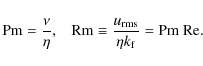
2.1 Units, nondimensional quantities, and parameters
Dimensionless quantities are obtained by setting
| (8) |
where
| [x] | = | ||
| [s] | = | (9) |
The simulations are then governed by the dimensionless numbers
 |
(10) |
where
 |
(11) |
with
The amount of stratification is determined by the parameter
 |
(12) |
where e0 is the internal energy at z4. We use
2.2 The test field method
We employ the test field method (Schrinner et al. 2005,2007), which is implemented into the P ENCIL C ODE, to determine turbulent transport coefficients. The uncurled induction equation in the shearing box approximation can be written in terms of the vector potential in the Weyl gauge as
where
 |
(14) |
In most cases we use
 |
(15) |
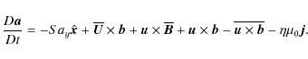
where the overbars denote a horizontal average and lowercase quantities denote fluctuations around these averages. The equation for the mean vector potential is then
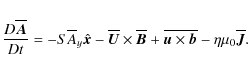
Subtracting (16) from (13) gives an equation for the fluctuating field which reads
Instead of using the actual mean fields
| (18) | |||
| (19) |
where k is the wavenumber of the test field. In most models we use k/k1=1, where
 |
(20) |
where
Owing to the use of periodic boundary conditions in the horizontal
directions, the z-component of the mean magnetic field is conserved
and equal to the initial value, i.e.
![]() .
Therefore the value of
.
Therefore the value of
![]() is here of no interest.
is here of no interest.
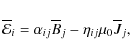
It is convenient to discuss the results in terms of the quantities
| |
= | (21) | |
| = | (22) | ||
| = | (23) |
Furthermore, the remaining or otherwise important coefficients are analyzed individually. The most important of these are the diagonal components of
Table 1:
Summary of the runs. The numbers are given for the statistically
saturated state. Here,
![]() ,
,
![]() ,
and
,
and
![]() .
.
To normalize our results, we use isotropic expressions of ![]() and
and
![]() as obtained from first order smoothing, i.e.
as obtained from first order smoothing, i.e.
 |
(24) |
where the root mean square velocity is a volume average and the Strouhal number,
| (25) |
has been assumed to be of the order of unity. In order to actually compare our results with those of FOSA, anisotropic expressions need to be used. Such expressions have been computed in the past (e.g. Rädler 1980; see also Käpylä et al. 2006a) and are given for the
where we have used integration by parts and assumed that
2.3 Averaging and error estimates
In the present study a mean quantity is considered to be a horizontal average, defined via
Except for special terms such as the shear terms in Eqs. (4) and (13), this formulation corresponds to simple horizontal averaging (for details see Brandenburg et al. 2008a). An additional time average over the statistically steady part of each simulations is also applied. The fluctuating magnetic fields bp,q are reset to zero after periodic time intervals in order to avoid the complications arising from the growth of these fields; see the more thorough discussions in Sur et al. (2008) and Mitra et al. (2009).
We estimate errors by computing the standard deviation ![]() for
each depth and dividing this by the square root of the number of
independent realizations N of the dynamo coefficients. We consider
the time series between two resets of the field
bp,q to
represent an independent realization. For a typical run, N is between five
and ten.
for
each depth and dividing this by the square root of the number of
independent realizations N of the dynamo coefficients. We consider
the time series between two resets of the field
bp,q to
represent an independent realization. For a typical run, N is between five
and ten.
2.4 Corresponding mean-field models
In order to determine how well the derived dynamo coefficients describe the dynamos seen in direct simulations of Paper I, we construct a one-dimensional mean-field model where the test field results can be used directly as inputs. We start from the mean-field induction equation, Eq. (1), which can be written using the vector potential |
(31) |
where the dot on
![\begin{figure}
\par\includegraphics[width=8cm,clip]{11498f01.eps}
\end{figure}](/articles/aa/full_html/2009/23/aa11498-08/img142.png) |
Figure 1:
The three topmost panels show the time-averaged vertical profiles of
kinetic helicity,
|
| Open with DEXTER | |
3 Results
In a similar fashion as in Paper I we perform four types of simulations which we label as follows: in set A neither rotation nor shear is present whereas in set B rotation is added. In set C only shear is present, and finally in set D both rotation and shear are used. Parameters such as the strengths of rotation and shear, as measured by
The fluid Reynolds numbers in our simulations are quite modest so we
cannot consider our flows to be highly turbulent. However, the flows are
irregular enough to remain time dependent in all cases, as can also
be seen from various animations![]() .
.
3.1 Set A: no rotation nor shear (Co = Sh = 0)
The simplest case we can consider with the present setup is one with no rotation and no shear. In that case no net helicity generation or
The horizontally and temporally averaged transport coefficients from
Run A with
![]() and
and
![]() are presented in
Fig. 1. The results show that the kinetic helicity
is small and that the mean values of the diagonal elements of
are presented in
Fig. 1. The results show that the kinetic helicity
is small and that the mean values of the diagonal elements of
![]() are of the order of
are of the order of
![]() with errors clearly larger than
the mean. Vanishing diagonal elements of
with errors clearly larger than
the mean. Vanishing diagonal elements of
![]() is
in accordance with expectations from symmetry arguments.
There is however a non-zero pumping effect directed upward (downward) in
the lower (upper) part of the convectively unstable layer. The sign of
the pumping is inconsistent with the diamagnetic effect, i.e.
is
in accordance with expectations from symmetry arguments.
There is however a non-zero pumping effect directed upward (downward) in
the lower (upper) part of the convectively unstable layer. The sign of
the pumping is inconsistent with the diamagnetic effect, i.e.
![]() (e.g. Rädler 1968) and differs from earlier results from convection
simulations using the imposed field method (Ossendrijver et al.
2002; Käpylä et al. 2006a)
and other diagnostics (e.g. Nordlund et al. 1992;
Tobias et al. 1998,2001; Ziegler & Rüdiger 2003).
However, this result is obtained for test fields for which k/k1=1,
whereas the imposed field results use a uniform field with
k/k1=0. For a uniform test field the pumping effect indeed changes
sign and is thus consistent with the earlier numerical studies and the
diamagnetic effect (see the upper panel
of Fig. 2).
The FOSA-prediction, Eq. (28) for the turbulent pumping is in qualitative
agreement with the simulation result for k/k1=0 but opposite to
the results for k/k1 greater than that.
(e.g. Rädler 1968) and differs from earlier results from convection
simulations using the imposed field method (Ossendrijver et al.
2002; Käpylä et al. 2006a)
and other diagnostics (e.g. Nordlund et al. 1992;
Tobias et al. 1998,2001; Ziegler & Rüdiger 2003).
However, this result is obtained for test fields for which k/k1=1,
whereas the imposed field results use a uniform field with
k/k1=0. For a uniform test field the pumping effect indeed changes
sign and is thus consistent with the earlier numerical studies and the
diamagnetic effect (see the upper panel
of Fig. 2).
The FOSA-prediction, Eq. (28) for the turbulent pumping is in qualitative
agreement with the simulation result for k/k1=0 but opposite to
the results for k/k1 greater than that.
![\begin{figure}
\par\includegraphics[width=7.2cm,clip]{11498f02.eps}
\par\end{figure}](/articles/aa/full_html/2009/23/aa11498-08/img145.png) |
Figure 2:
Coefficients |
| Open with DEXTER | |
At first glance the magnitude of the turbulent diffusivity seems quite high: the
maximum value is more than six times the isotropic reference value
![]() suggesting that
suggesting that
![]() .
However, the high value of
.
However, the high value of
![]() turns out to be related to the
normalization: if an anisotropic expression, i.e. Eq. (29), is plotted alongside
turns out to be related to the
normalization: if an anisotropic expression, i.e. Eq. (29), is plotted alongside
![]() the Strouhal
number is roughly 1.6, not six, for our standard case k/k1=1,
see the lower panel of
Fig. 2. The profile of the turbulent diffusivity
coincides with that of the vertical velocity squared as predicted by
Eq. (29).
When k is increased, the profile of
the Strouhal
number is roughly 1.6, not six, for our standard case k/k1=1,
see the lower panel of
Fig. 2. The profile of the turbulent diffusivity
coincides with that of the vertical velocity squared as predicted by
Eq. (29).
When k is increased, the profile of
![]() stays roughly the same
and the magnitude diminishes roughly in proportion to k-1.
The quantities
stays roughly the same
and the magnitude diminishes roughly in proportion to k-1.
The quantities
![]() ,
,
![]() ,
,
![]() ,
,
![]() ,
and
,
and ![]() are compatible with zero in all runs in set A.
are compatible with zero in all runs in set A.
![\begin{figure}
\par\includegraphics[width=8cm,clip]{11498f03.eps}
\end{figure}](/articles/aa/full_html/2009/23/aa11498-08/img149.png) |
Figure 3:
Same as Fig. 1, but for Run B;
|
| Open with DEXTER | |
![\begin{figure}
\par\includegraphics[width=7.8cm,clip]{11498f04.eps}
\end{figure}](/articles/aa/full_html/2009/23/aa11498-08/img150.png) |
Figure 4:
From top to bottom: kinetic helicity,
|
| Open with DEXTER | |
![\begin{figure}
\par\includegraphics[width=8cm,clip]{11498f05.eps}
\end{figure}](/articles/aa/full_html/2009/23/aa11498-08/img151.png) |
Figure 5:
From top to bottom: kinetic helicity,
|
| Open with DEXTER | |
![\begin{figure}
\par\includegraphics[width=8cm,clip]{11498f06.eps}
\end{figure}](/articles/aa/full_html/2009/23/aa11498-08/img152.png) |
Figure 6:
From top to bottom: |
| Open with DEXTER | |
![\begin{figure}
\par\includegraphics[width=8cm,clip]{11498f07.eps}
\end{figure}](/articles/aa/full_html/2009/23/aa11498-08/img154.png) |
Figure 7:
From top to bottom: kinetic helicity, |
| Open with DEXTER | |
3.2 Set B: only rotation (Co  0, Sh = 0)
When rotation (corresponding to the north pole,
In comparison to Run A,
the pumping coefficient ![]() shows a deeper maximum in the upper
half of the convection zone and somewhat decreased value in the lower
half. The profile and magnitude of the turbulent diffusivity are
similar to those in the nonrotating case. The
coefficients
shows a deeper maximum in the upper
half of the convection zone and somewhat decreased value in the lower
half. The profile and magnitude of the turbulent diffusivity are
similar to those in the nonrotating case. The
coefficients ![]() and
and ![]() are equal in magnitude and of
opposite sign. This leads to a positive (negative)
are equal in magnitude and of
opposite sign. This leads to a positive (negative) ![]() in the
convection zone (overshoot layer) with magnitude peaking close to twice
in the
convection zone (overshoot layer) with magnitude peaking close to twice
![]() .
The quantities
.
The quantities
![]() and
and
![]() are small, as expected from symmetry arguments
are small, as expected from symmetry arguments
3.2.1 Dependence on horizontal system size
The profiles and magnitudes of the two diagonal components of
3.2.2 Dependence on Rm
One of the basic expected properties of turbulent dynamos is that they should be ``fast'', i.e. the growth rate of the dynamo, and thus the transport coefficients, should not depend on the molecular magnetic diffusion provided that
3.2.3 Dependence on wavenumber k
The results for nonrotating convection (see Fig. 2) indicate that at least the pumping effect can experience not only a change in magnitude but also a qualitative change when the wavenumber of the test field is varied (for corresponding details see Brandenburg et al. 2008b). It is of great interest to study whether similar effects can occur for the
3.2.4 Dependence on Co
The
Interestingly, the turbulent diffusivity shows a
marked decrease for rapid rotation.
The coefficient ![]() is positive in the convection zone and
negative in the overshoot layer for slow rotation. The magnitude increases
rapidly until
is positive in the convection zone and
negative in the overshoot layer for slow rotation. The magnitude increases
rapidly until
![]() ,
after which
,
after which ![]() changes sign near
the top. This negative region increases with rotation. Similar
results, i.e. monotonically decreasing
changes sign near
the top. This negative region increases with rotation. Similar
results, i.e. monotonically decreasing
![]() and a first increasing
and then decreasing
and a first increasing
and then decreasing ![]() were obtained from forced turbulence
simulations by Brandenburg et al. (2008a).
were obtained from forced turbulence
simulations by Brandenburg et al. (2008a).
The combined effect of increasing ![]() and decreasing
and decreasing
![]() suggests that the large-scale dynamo was possibly subcritical in the
runs with only rotation in Paper I and other earlier studies (e.g.
Nordlund et al. 1992; Brandenburg et al. 1996;
Cattaneo & Hughes 2006; Tobias et al. 2008),
but that it could be excited for
more rapid rotation. The validity of this conjecture is given some
credibility by Käpylä et al. (2009a) who find clear
large-scale dynamo action for
suggests that the large-scale dynamo was possibly subcritical in the
runs with only rotation in Paper I and other earlier studies (e.g.
Nordlund et al. 1992; Brandenburg et al. 1996;
Cattaneo & Hughes 2006; Tobias et al. 2008),
but that it could be excited for
more rapid rotation. The validity of this conjecture is given some
credibility by Käpylä et al. (2009a) who find clear
large-scale dynamo action for
![]() for a similar setup as used here
and in Paper I. More detailed discussion of these results can be found
in the aforementioned reference.
for a similar setup as used here
and in Paper I. More detailed discussion of these results can be found
in the aforementioned reference.
3.2.5 Dependence on 
The latitude dependence of the coefficients for
![\begin{figure}
\par\includegraphics[width=8cm,clip]{11498f08.eps}
\end{figure}](/articles/aa/full_html/2009/23/aa11498-08/img170.png) |
Figure 8:
From top to bottom: kinetic helicity,
|
| Open with DEXTER | |
![\begin{figure}
\par\includegraphics[width=8.2cm,clip]{11498f09.eps}
\end{figure}](/articles/aa/full_html/2009/23/aa11498-08/img171.png) |
Figure 9:
Same as Fig. 1, but for Run C with no rotation
and just shear;
|
| Open with DEXTER | |
![\begin{figure}
\par\includegraphics[width=8.2cm,clip]{11498f10.eps}
\end{figure}](/articles/aa/full_html/2009/23/aa11498-08/img172.png) |
Figure 10:
From top to bottom: kinetic helicity,
|
| Open with DEXTER | |
3.3 Set C: only shear (Co = 0, Sh
0)
3.3.1 Simulation results
The next case to consider is that of shear only. We use uniform shear of the form
The turbulent pumping in Run C has a similar profile as in the cases with
![]() (Run A) and
(Run A) and
![]() (Run B) with k/k1=1 with
downward pumping near the surface and
upward pumping in the lower part of the convectively unstable region.
The profile and magnitude of the turbulent diffusivity is also very
similar to previous cases.
The pumping effect and turbulent diffusivity are
decreased when the magnitude of
(Run B) with k/k1=1 with
downward pumping near the surface and
upward pumping in the lower part of the convectively unstable region.
The profile and magnitude of the turbulent diffusivity is also very
similar to previous cases.
The pumping effect and turbulent diffusivity are
decreased when the magnitude of ![]() is greater than 0.06. The
results for increasing
is greater than 0.06. The
results for increasing ![]() and decreasing
and decreasing
![]() as functions of
shear are opposite to those obtained from helically forced turbulence
with shear (Mitra et al. 2009).
However, the comparison for the
as functions of
shear are opposite to those obtained from helically forced turbulence
with shear (Mitra et al. 2009).
However, the comparison for the ![]() -effect should be done with
caution because in Mitra et al. (2009)
-effect should be done with
caution because in Mitra et al. (2009) ![]() arises
essentially due to the external forcing and is only modified by the
action of shear whereas in the present case
arises
essentially due to the external forcing and is only modified by the
action of shear whereas in the present case ![]() is due to the
interaction of shear, stratification, and turbulence themselves.
is due to the
interaction of shear, stratification, and turbulence themselves.
The ![]() component, which can drive a mean-field shear-current
dynamo for
component, which can drive a mean-field shear-current
dynamo for
![]() ,
is of interest because it can
provide an explanation for the dynamos seen in recent dynamo
simulations (Paper I; Hughes & Proctor 2009). In the present
case where S<0,
,
is of interest because it can
provide an explanation for the dynamos seen in recent dynamo
simulations (Paper I; Hughes & Proctor 2009). In the present
case where S<0, ![]() should be negative to excite the
shear-current dynamo. There appear to be consistently negative regions
of
should be negative to excite the
shear-current dynamo. There appear to be consistently negative regions
of ![]() at the interface of the convectively unstable region
and the overshoot layer, and in the upper layers of the convection
zone. The upper negative region is more pronounced for
at the interface of the convectively unstable region
and the overshoot layer, and in the upper layers of the convection
zone. The upper negative region is more pronounced for
![]() and
and
![]() .
However, the errors of these quantities are of the
same order of magnitude as the mean value, cf. the bottom panel of
Fig. 9. These results tend to agree with earlier
findings from forced turbulence (Brandenburg et al. 2008a;
Mitra et al. 2009)
where
.
However, the errors of these quantities are of the
same order of magnitude as the mean value, cf. the bottom panel of
Fig. 9. These results tend to agree with earlier
findings from forced turbulence (Brandenburg et al. 2008a;
Mitra et al. 2009)
where ![]() for the most part was positive or compatible with
zero.
for the most part was positive or compatible with
zero.
![\begin{figure}
\par\includegraphics[width=8cm,clip]{11498f11.eps}
\end{figure}](/articles/aa/full_html/2009/23/aa11498-08/img180.png) |
Figure 11:
Growth rates |
| Open with DEXTER | |
3.3.2 Mean-field dynamo models
In Paper I clear large-scale dynamo action was found from a simulation with
Using the full test field results for
![]() and
and ![]() in the
corresponding mean-field model indicates that a dynamo is excited for
in the
corresponding mean-field model indicates that a dynamo is excited for
![]() ,
see the growth rates of the large-scale field presented Fig. 11.
It is interesting to study what are the relative importances of the
different effects: first we turn off the off-diagonal components of
,
see the growth rates of the large-scale field presented Fig. 11.
It is interesting to study what are the relative importances of the
different effects: first we turn off the off-diagonal components of
![]() in which case the magnetic field is generated by the
in which case the magnetic field is generated by the
![]() -effect and the shear-current effect is absent. We find that
the growth rate decreases but is still positive for the same cases as
before. On the other hand, a ``pure'' shear-current dynamo, i.e. where
-effect and the shear-current effect is absent. We find that
the growth rate decreases but is still positive for the same cases as
before. On the other hand, a ``pure'' shear-current dynamo, i.e. where
![]() ,
is also excited
for the same runs with a very similar
,
is also excited
for the same runs with a very similar ![]() as in the
as in the
![]() -shear case. In comparison to the simulations of Paper I, we
find that the growth rates from the mean-field model are consistently
significantly smaller. These results and the fact that no dynamo was
found for
-shear case. In comparison to the simulations of Paper I, we
find that the growth rates from the mean-field model are consistently
significantly smaller. These results and the fact that no dynamo was
found for
![]() would seem to indicate that an incoherent
would seem to indicate that an incoherent
![]() -shear dynamo (e.g. Vishniac & Brandenburg 1997) is
also operating in the full simulations. However, we should remain
cautious when comparing the direct simulations and the mean-field model
because the transport coefficients were determined for a single value
of k whereas many other wavenumbers are available in the
simulations.
-shear dynamo (e.g. Vishniac & Brandenburg 1997) is
also operating in the full simulations. However, we should remain
cautious when comparing the direct simulations and the mean-field model
because the transport coefficients were determined for a single value
of k whereas many other wavenumbers are available in the
simulations.
![\begin{figure}
\par\includegraphics[width=8cm,clip]{11498f12.eps}
\end{figure}](/articles/aa/full_html/2009/23/aa11498-08/img187.png) |
Figure 12:
Same as Fig. 1, but for Run D with both rotation
and shear;
|
| Open with DEXTER | |
3.4 Set D: rotation and shear (Co
0, Sh
0)
3.4.1 Simulation results
When rotation is added to the system where a large-scale shear is already imposed, the vorticity generation is suppressed (e.g. Yousef et al. 2008b; Paper I) and it is possible to study higher values of
We note that in a recent paper, Hughes & Proctor (2009) found that the
![]() -effect is virtually unchanged when shear is added to a
rotating system. In their case the shear profile is proportional to
-effect is virtually unchanged when shear is added to a
rotating system. In their case the shear profile is proportional to
![]() .
The resulting large-scale vorticity is then
.
The resulting large-scale vorticity is then
![]() which leads to
which leads to
![]() (e.g. Rädler &
Stepanov 2006) where G symbolically denotes the
inhomogeneity of the turbulence. However, Hughes & Proctor
(2009) show a volume average of
(e.g. Rädler &
Stepanov 2006) where G symbolically denotes the
inhomogeneity of the turbulence. However, Hughes & Proctor
(2009) show a volume average of ![]() over the full upper half
of the domain in which case the contribution of
over the full upper half
of the domain in which case the contribution of
![]() cancels out.
This explains the absence of any modifications of
cancels out.
This explains the absence of any modifications of ![]() due to shear in their case, but for us this is not the case because for
our shear profile
due to shear in their case, but for us this is not the case because for
our shear profile
![]() .
.
The profile of ![]() is quite similar to the rotating case, i.e. Run B; see Fig. 3, with the exception that the
off-diagonal components of
is quite similar to the rotating case, i.e. Run B; see Fig. 3, with the exception that the
off-diagonal components of
![]() show considerable anisotropy
as manifested by the parameter
show considerable anisotropy
as manifested by the parameter
![]() .
The turbulent
diffusion shows a profile common to all the other simulations, but
here the diagonal components of
.
The turbulent
diffusion shows a profile common to all the other simulations, but
here the diagonal components of ![]() show evidence of mild anisotropy with
show evidence of mild anisotropy with
![]() peaking near the middle of the convectively unstable
region with a maximum value of
peaking near the middle of the convectively unstable
region with a maximum value of
![]() .
The
quantity
.
The
quantity ![]() is compatible with zero whereas
is compatible with zero whereas ![]() exhibits
a similar profile and magnitude as
exhibits
a similar profile and magnitude as ![]() does in the rotating
case, cf. Fig. 3, which indicates that
does in the rotating
case, cf. Fig. 3, which indicates that
![]() ,
as opposed to
,
as opposed to
![]() in Run B.
in Run B.
The kinetic helicity and the turbulent transport coefficients as functions of
![]() ,
keeping the ratio
,
keeping the ratio
![]() constant, are shown in
Fig. 13. The helicity is increasing in a similar
fashion as, albeit slower than, in the absence of shear, compare with
Fig. 7. The components of the
constant, are shown in
Fig. 13. The helicity is increasing in a similar
fashion as, albeit slower than, in the absence of shear, compare with
Fig. 7. The components of the ![]() -effect are
highly anisotropic with the main contribution of
-effect are
highly anisotropic with the main contribution of
![]() being
due to shear and that of
being
due to shear and that of
![]() due to rotation (compare with
Figs. 7 and 10). The value of
due to rotation (compare with
Figs. 7 and 10). The value of
![]() is somewhat decreased in comparison to the cases with
shear only whereas
is somewhat decreased in comparison to the cases with
shear only whereas
![]() is almost unaffected. This is in
qualitative agreement with adding the contributions of runs
from Sets B and C with corresponding
is almost unaffected. This is in
qualitative agreement with adding the contributions of runs
from Sets B and C with corresponding ![]() and
and ![]() ,
respectively.
,
respectively.
![\begin{figure}
\par\includegraphics[width=8cm,clip]{11498f13.eps}
\end{figure}](/articles/aa/full_html/2009/23/aa11498-08/img197.png) |
Figure 13:
From top to bottom: kinetic helicity,
|
| Open with DEXTER | |
The profiles of ![]() and
and
![]() are similar to those
with only
rotation. The differences of
are similar to those
with only
rotation. The differences of ![]() and
and
![]() as a function of
as a function of
![]() are small and for the most part fall within the error bars.
The profile of
are small and for the most part fall within the error bars.
The profile of ![]() is very similar to
is very similar to ![]() in the case of only
rotation with negative values near the base and top of the
convectively unstable region with positive values in between.
The profile and magnitude of
in the case of only
rotation with negative values near the base and top of the
convectively unstable region with positive values in between.
The profile and magnitude of ![]() remains essentially fixed for
remains essentially fixed for
![]() .
We note that in the simulations with shear and rotation the
.
We note that in the simulations with shear and rotation the
![]() -effect may also contribute to the
generation of large-scale magnetic fields (e.g. Rädler 1969;
Rädler et al. 2003; Pipin et al. 2008). It is,
however, not altogether clear how to disentangle the transport
coefficients responsible for the shear-current and
-effect may also contribute to the
generation of large-scale magnetic fields (e.g. Rädler 1969;
Rädler et al. 2003; Pipin et al. 2008). It is,
however, not altogether clear how to disentangle the transport
coefficients responsible for the shear-current and
![]() -dynamos in the present case. Thus the
off-diagonal components of
-dynamos in the present case. Thus the
off-diagonal components of ![]() contain contributions from
both effects in Set D.
contain contributions from
both effects in Set D.
3.4.2 Mean-field dynamo models
We follow here the same procedure as in Sect. 3.3.2 to study dynamo excitation for the Runs D1-D5. Using the full
![\begin{figure}
\par\includegraphics[width=8cm,clip]{11498f14.eps}
\end{figure}](/articles/aa/full_html/2009/23/aa11498-08/img202.png) |
Figure 14: |
| Open with DEXTER | |
4 Conclusions
We obtain turbulent transport coefficients governing the evolution of large-scale magnetic fields from turbulent convection simulations with the test field method. We study the system size and magnetic Reynolds number dependences of the coefficients. This is important because spurious results can be expected for small Reynolds numbers or when the aspect ratio of the domain is too small (Hughes & Cattaneo 2008). We find that for our standard system size,
The earlier determinations of transport coefficients from convection
simulations have used the imposed field method (e.g. Ossendrijver et al. 2001,2002; Käpylä et al. 2006a) which
yields the components of
![]() but does not deliver
but does not deliver
![]() because the imposed field is uniform. The test field
method does not suffer from this restriction and
because the imposed field is uniform. The test field
method does not suffer from this restriction and ![]() and the
k-dependence of the coefficients can be extracted. We find that for
k/k1=0, i.e. for a uniform field, the results for
and the
k-dependence of the coefficients can be extracted. We find that for
k/k1=0, i.e. for a uniform field, the results for ![]() and
and
![]() are consistent with those obtained from imposed field
calculations, provided the magnetic field is reset before it grows
too large and substantial gradients develop.
As k is increased, however, the qualitative behaviour
of the coefficients changes. This is indicated by a partial
sign change of
are consistent with those obtained from imposed field
calculations, provided the magnetic field is reset before it grows
too large and substantial gradients develop.
As k is increased, however, the qualitative behaviour
of the coefficients changes. This is indicated by a partial
sign change of ![]() and a complete sign change of
and a complete sign change of ![]() ;
see
Figs. 2 and 6.
;
see
Figs. 2 and 6.
The turbulent diffusivity shows a robust behaviour regardless of
the parameters of the simulations: the profile is proportional to the
vertical velocity squared,
![]() ,
as predicted by FOSA (e.g. Rädler 1980). The value of
,
as predicted by FOSA (e.g. Rädler 1980). The value of
![]() decreases almost
proportional to k-1, and shows a declining trend as a function
of rotation and shear.
decreases almost
proportional to k-1, and shows a declining trend as a function
of rotation and shear.
For the present parameters,
the ![]() -effect increases monotonically as rotation is increased.
As a function of latitude, the diagonal components of
-effect increases monotonically as rotation is increased.
As a function of latitude, the diagonal components of
![]() have a similar magnitude and peak near the pole with declining values
towards the equator. The
have a similar magnitude and peak near the pole with declining values
towards the equator. The ![]() -effect induced by shear is highly
anisotropic: the
-effect induced by shear is highly
anisotropic: the
![]() component has a similar profile and
magnitude, but opposite sign, as
component has a similar profile and
magnitude, but opposite sign, as
![]() and
and
![]() in the case of only
rotation. This component also increases monotonically as a function of
shear, whereas the shear-induced
in the case of only
rotation. This component also increases monotonically as a function of
shear, whereas the shear-induced
![]() remains small
regardless of the strength of the shear. In the runs where rotation
and shear are present, the diagonal components of
remains small
regardless of the strength of the shear. In the runs where rotation
and shear are present, the diagonal components of
![]() are
roughly the sums of the corresponding coefficients in the cases with
rotation and shear alone.
are
roughly the sums of the corresponding coefficients in the cases with
rotation and shear alone.
In addition to the ![]() -effect, the
-effect, the ![]() component can contribute
to a shear-current dynamo when
component can contribute
to a shear-current dynamo when
![]() .
In our case, where S<0,
such dynamo action is possible if
.
In our case, where S<0,
such dynamo action is possible if
![]() .
We find that this
coefficient shows negative regions near the base and near the top of the
convectively unstable region, but the errors are of the same order
of magnitude as the negative mean values in most cases.
.
We find that this
coefficient shows negative regions near the base and near the top of the
convectively unstable region, but the errors are of the same order
of magnitude as the negative mean values in most cases.
In order to connect to earlier work, we use the test field results in
a one-dimensional mean-field model in order to understand the
excitation of dynamos using identical setups as in direct simulations
(Paper I). We study here only the cases with shear and
consider large-scale dynamos in the rigidly rotating case elsewhere
(Käpylä et al. 2009a).
The presently used dynamo model ignores k-dependence and is therefore
likely to be too simple to fully describe the large-scale fields in the
direct simulations. Nevertheless, the present results, taken at face value,
seem to indicate that in the case with shear alone the derived dynamo
coefficients are not sufficient to explain the dynamo but that an
additional incoherent ![]() -shear dynamo might be needed. This
conjecture is based on the fact that mean-field
-shear dynamo might be needed. This
conjecture is based on the fact that mean-field ![]() -shear and
shear-current dynamos are both excited with similar growth rates
which, however, are significantly smaller than those obtained from
direct simulations in Paper I.
Furthermore, a large-scale dynamo was marginal for
-shear and
shear-current dynamos are both excited with similar growth rates
which, however, are significantly smaller than those obtained from
direct simulations in Paper I.
Furthermore, a large-scale dynamo was marginal for
![]() in
Paper I, whereas for
in
Paper I, whereas for
![]() it was found to be slightly subcritical in the
present study.
On the other hand, for the case with both shear and rotation, no
additional incoherent effects seem to be needed. We find that in this
case the regular
it was found to be slightly subcritical in the
present study.
On the other hand, for the case with both shear and rotation, no
additional incoherent effects seem to be needed. We find that in this
case the regular ![]() -shear dynamo produces larger growth rates
than the combined shear-current and
-shear dynamo produces larger growth rates
than the combined shear-current and
![]() dynamo but neither effect alone seems to be
strong enough to explain the dynamos in Paper I.
dynamo but neither effect alone seems to be
strong enough to explain the dynamos in Paper I.
On a more general level, mean-field dynamo models of the Sun and other
stars rely on parameterisations of turbulent transport
coefficients. Even today, the majority of solar dynamo models bypass
this problem and ignore most of the turbulent effects and rely on
phenomenological descriptions of the ![]() -effect and turbulent
diffusion that are not without problems theoretically. On the other
hand, some attempts have been made to incorporate the results for the
transport coefficients from imposed field studies in mean-field models
of the solar magnetism (e.g. Käpylä et al. 2006b;
Guerrero & de Gouveia Dal Pino 2008) and
models employing more general turbulence models have recently appeared
(e.g. Pipin & Seehafer 2009). We feel that this is a worthy cause to
follow further with the present results.
-effect and turbulent
diffusion that are not without problems theoretically. On the other
hand, some attempts have been made to incorporate the results for the
transport coefficients from imposed field studies in mean-field models
of the solar magnetism (e.g. Käpylä et al. 2006b;
Guerrero & de Gouveia Dal Pino 2008) and
models employing more general turbulence models have recently appeared
(e.g. Pipin & Seehafer 2009). We feel that this is a worthy cause to
follow further with the present results.
Acknowledgements
The authors wish to acknowledge the anonymous referee and Prof. Gunther Rüdiger for their helpful comments on the manuscript. The computations were performed on the facilities hosted by CSC - IT Center for Science in Espoo, Finland, who are administered by the Finnish ministry of education. This research has greatly benefitted from the computational resources granted by the CSC to the grand challenge project ``Dynamo08''. Financial support from the Academy of Finland grants No. 121431 (PJK) and 112020 (MJK) and the Swedish Research Council grant 621-2007-4064 (AB) is acknowledged, The authors acknowledge the hospitality of Nordita during the program ``Turbulence and Dynamos'' during which this work was initiated.
References
- Brandenburg, A. 2001, ApJ, 550, 824 [NASA ADS] [CrossRef] (In the text)
- Brandenburg, A. 2005a, ApJ, 625, 539 [NASA ADS] [CrossRef]
- Brandenburg, A. 2005b, AN, 326, 787 [NASA ADS] (In the text)
- Brandenburg, A. 2008, AN, 329, 725 [NASA ADS]
- Brandenburg, A., & Käpylä, P. J. 2007, NJP, 9, 305 [NASA ADS] [CrossRef] (In the text)
- Brandenburg, A., & Subramanian, K. 2005, Phys. Rep., 417, 1 [NASA ADS] [CrossRef] (In the text)
- Brandenburg, A., Tuominen, I., Nordlund, Å., et al. 1990, A&A, 232, 277 [NASA ADS] (In the text)
- Brandenburg, A., Nordlund, Å., Stein, R. F., & Torkelsson, U. 1995, ApJ, 446, 741 [NASA ADS] [CrossRef] (In the text)
- Brandenburg, A., Jennings, R. L., Nordlund, Å., et al. 1996, JFM, 306, 325 [NASA ADS] [CrossRef] (In the text)
- Brandenburg, A., Bigazzi, A., & Subramanian, K. 2001, MNRAS, 325, 685 [NASA ADS] [CrossRef] (In the text)
- Brandenburg, A., Rädler, K.-H., Rheinhardt, M., & Käpylä, P. J. 2008a, ApJ, 676, 740 [NASA ADS] [CrossRef] (In the text)
- Brandenburg, A., Rädler, K.-H., & Schrinner, M. 2008b, A&A, 482, 739 [NASA ADS] [CrossRef] [EDP Sciences] (In the text)
- Brown, B. P., Browning, M. K., Brun, A. S., et al. 2007, AIPC, 948, 271 [NASA ADS] (In the text)
- Browning, M. K., Miesch, M. S., Brun, A. S., & Toomre, J. 2006, ApJ, 648, L157 [NASA ADS] [CrossRef] (In the text)
- Cattaneo, F., & Hughes, D. W. 2006, JFM, 553, 401 [NASA ADS] [CrossRef] (In the text)
- Elperin, T., Kleeorin, N., & Rogachevskii, I. 2003, PhRvE, 68, 016311 [NASA ADS] (In the text)
- Giesecke, A., Ziegler, U., & Rüdiger, G. 2005, Phys. Earth Planet. Interiors, 152, 90 [NASA ADS] [CrossRef] (In the text)
- Gressel, O., Ziegler, U., Elstner, D., & Rüdiger, G. 2008, AN, 329, 619 [NASA ADS] 401 (In the text)
- Guerrero, G., & de Gouveia Dal Pino, E. M. 2008, A&A, 485, 267 [NASA ADS] [CrossRef] [EDP Sciences] (In the text)
- Hughes, D. W., & Cattaneo, F. 2008, JFM, 594, 445 (In the text)
- Hughes, D. W., & Proctor, M. R. E. 2009, PhRvL, 102, 044501 [NASA ADS] (In the text)
- Hawley, J. F., Gammie, C. F., & Balbus, S.A. 1996, ApJ, 464, 690 [NASA ADS] [CrossRef] (In the text)
- Käpylä, P. J., & Brandenburg, A. 2009, ApJ, in press [arXiv:0810.2298] (In the text)
- Käpylä, P. J., Korpi, M. J., & Tuominen, I. 2004, A&A, 422, 793 [NASA ADS] [CrossRef] [EDP Sciences] (In the text)
- Käpylä, P. J., Korpi, M. J., Ossendrijver, M., & Stix, M. 2006a, A&A, 455, 401 [NASA ADS] [CrossRef] [EDP Sciences] (In the text)
- Käpylä, P. J., Korpi, M. J., & Tuominen, I. 2006b, AN, 327, 884 [NASA ADS] (In the text)
- Käpylä, P. J., Korpi, M. J., & Brandenburg, A. 2008, A&A, 491, 353 [NASA ADS] [CrossRef] [EDP Sciences] (Paper I) (In the text)
- Käpylä, P. J., Korpi, M. J., & Brandenburg, A. 2009a, ApJ, 697, 1153 [NASA ADS] [CrossRef] (In the text)
- Käpylä, P. J., Mitra, D., & Brandenburg, A. 2009b, PhRvE, 79, 016302 [NASA ADS] (In the text)
- Kleeorin, N., & Rogachevskii, I. 2008, PhRvE, 77, 036307 [NASA ADS] (In the text)
- Krause, F., & Rädler, K.-H. 1980, Mean-field Magnetohydrodynamics and Dynamo Theory (Oxford: Pergamon Press) (In the text)
- Mininni, P. D., Gómez, D. O., & Mahajan, S. M. 2005, ApJ, 619, 1019 [NASA ADS] [CrossRef] (In the text)
- Mitra, D., Käpylä, P. J., Tavakol, R., & Brandenburg, A. 2009, A&A, 495, 1 [NASA ADS] [CrossRef] [EDP Sciences] (In the text)
- Moffatt, H. K. 1978, Magnetic field generation in electrically conducting fluids (Cambridge: Cambridge Univ. Press) (In the text)
- Nordlund, Å, Brandenburg, A., Jennings, R. L., et al. 1992, ApJ, 392, 647 [NASA ADS] [CrossRef] (In the text)
- Ossendrijver, M. 2003, A&AR, 11, 287 [NASA ADS] (In the text)
- Ossendrijver, M., Stix, M., & Brandenburg, A. 2001, A&A, 376, 726 [NASA ADS] [CrossRef] (In the text)
- Ossendrijver, M., Stix, M., Rüdiger, G., & Brandenburg, A. 2002, A&A, 394, 735 [NASA ADS] [CrossRef] [EDP Sciences] (In the text)
- Parker, E. N. 1979, Cosmical Magnetic Fields: Their Origin and Their Activity (Oxford, NY: Clarendon Press) (In the text)
- Pipin, V. V. 2008, GAFD, 102, 21 [CrossRef] (In the text)
- Pipin, V. V., & Seehafer, N. 2009, A&A, 493, 819 [NASA ADS] [CrossRef] [EDP Sciences] (In the text)
- Proctor, M. R. E. 2007, MNRAS, 382, 39 [NASA ADS] (In the text)
- Rädler, K.-H. 1968, Z. Naturforsch., 23a, 1851 [NASA ADS] (In the text)
- Rädler, K.-H. 1969, Monatsber. Dtsch. Akad. Wiss. Berlin, 11, 194 (In the text)
- Rädler, K.-H. 1980, AN, 301, 101 [NASA ADS] (In the text)
- Rädler, K.-H., & Stepanov, R. 2006, PhRvE, 73, 056311 [NASA ADS] (In the text)
- Rädler, K.-H., Kleeorin, N., & Rogachevskii, I. 2003, GAFD, 97, 249 [CrossRef] (In the text)
- Rogachevskii, I., & Kleeorin, N. 2003, PhRvE, 68, 036301 [NASA ADS] (In the text)
- Rogachevskii, I., & Kleeorin, N. 2004, PhRvE, 70, 046310 [NASA ADS]
- Rotvig, J., & Jones, C. A. 2002, PhRvE, 66, 056308 [NASA ADS] (In the text)
- Rüdiger, G., & Hollerbach, R. 2004, The magnetic Universe (Weinheim: Wiley-VCH) (In the text)
- Rüdiger, G., & Kitchatinov, L. L. 2006, AN, 327, 298 [NASA ADS] (In the text)
- Schrinner, M., Rädler, K.-H., Schmitt, D., et al. 2005, AN, 326, 245 [NASA ADS] (In the text)
- Schrinner, M., Rädler, K.-H., Schmitt, D., et al. 2007, GAFD, 101, 81 [CrossRef]
- Sur, S., Brandenburg, A., & Subramanian, K. 2008, MNRAS, 385, L15 [NASA ADS] (In the text)
- Tobias, S. M., Brummell, N. H., Clune, Th. L., & Toomre, J. 1998, ApJ, 502, L177 [NASA ADS] [CrossRef] (In the text)
- Tobias, S. M., Brummell, N. H., Clune, Th. L., & Toomre, J. 2001, ApJ, 549, 1183 [NASA ADS] [CrossRef]
- Tobias, S. M., Cattaneo, F., & Brummell, N. H. 2008, ApJ, 685, 596 [NASA ADS] [CrossRef] (In the text)
- Vainshtein, S. I., & Cattaneo, F. 1992, ApJ, 393, 165 [NASA ADS] [CrossRef] (In the text)
- Vishniac, E. T., & Brandenburg, A. 1997, ApJ, 475, 263 [NASA ADS] [CrossRef] (In the text)
- Vishniac, E. T., & Cho, J. 2001, ApJ, 550, 752 [NASA ADS] [CrossRef] (In the text)
- Yousef, T. A., Heinemann, T., Schekochihin, A. A., et al. 2008a, PhRvL, 100, 184501 [NASA ADS] (In the text)
- Yousef, T. A., Heinemann, T., Rincon, F., et al. 2008b, AN, 329, 737 [NASA ADS] (In the text)
- Ziegler, U., & Rüdiger, G. 2003, A&A, 401, 433 [NASA ADS] [CrossRef] [EDP Sciences] (In the text)
Footnotes
- ... ODE
![[*]](/icons/foot_motif.png)
- http://www.nordita.org/software/pencil-code/
- ... animations
- http://www.helsinki.fi/kapyla/movies.html
- ... number
- The
definition of Coriolis number in the present study is smaller by a factor of
 in comparison to previous studies.
All Tables
Table 1:
Summary of the runs. The numbers are given for the statistically
saturated state. Here,
![]() ,
,
![]() ,
and
,
and
![]() .
.
All Figures
| |
Figure 1:
The three topmost panels show the time-averaged vertical profiles of
kinetic helicity,
|
| Open with DEXTER | |
| In the text | |
| |
Figure 2:
Coefficients |
| Open with DEXTER | |
| In the text | |
| |
Figure 3:
Same as Fig. 1, but for Run B;
|
| Open with DEXTER | |
| In the text | |
| |
Figure 4:
From top to bottom: kinetic helicity,
|
| Open with DEXTER | |
| In the text | |
| |
Figure 5:
From top to bottom: kinetic helicity,
|
| Open with DEXTER | |
| In the text | |
| |
Figure 6:
From top to bottom: |
| Open with DEXTER | |
| In the text | |
| |
Figure 7:
From top to bottom: kinetic helicity, |
| Open with DEXTER | |
| In the text | |
| |
Figure 8:
From top to bottom: kinetic helicity,
|
| Open with DEXTER | |
| In the text | |
| |
Figure 9:
Same as Fig. 1, but for Run C with no rotation
and just shear;
|
| Open with DEXTER | |
| In the text | |
| |
Figure 10:
From top to bottom: kinetic helicity,
|
| Open with DEXTER | |
| In the text | |
| |
Figure 11:
Growth rates |
| Open with DEXTER | |
| In the text | |
| |
Figure 12:
Same as Fig. 1, but for Run D with both rotation
and shear;
|
| Open with DEXTER | |
| In the text | |
| |
Figure 13:
From top to bottom: kinetic helicity,
|
| Open with DEXTER | |
| In the text | |
| |
Figure 14: |
| Open with DEXTER | |
| In the text | |
Copyright ESO 2009
Current usage metrics show cumulative count of Article Views (full-text article views including HTML views, PDF and ePub downloads, according to the available data) and Abstracts Views on Vision4Press platform.
Data correspond to usage on the plateform after 2015. The current usage metrics is available 48-96 hours after online publication and is updated daily on week days.
Initial download of the metrics may take a while.