| Issue |
A&A
Volume 500, Number 2, June III 2009
|
|
|---|---|---|
| Page(s) | 781 - 784 | |
| Section | Galactic structure, stellar clusters, and populations | |
| DOI | https://doi.org/10.1051/0004-6361/200809404 | |
| Published online | 01 April 2009 | |
Potential-density pairs and vertical tilt of the stellar velocity ellipsoid
O. Bienaymé
Université de Strasbourg, CNRS, Observatoire Astronomique, France
Received 16 January 2008 / Accepted 9 March 2009
Abstract
We define new potential-density pairs and examine the
impact of the potential flattening on the vertical velocity ellipsoid
tilt, ![]() .
By means of numerical integrations and analytical
calculations, we estimate
.
By means of numerical integrations and analytical
calculations, we estimate ![]() in a variety of galactic
potentials. We show that at 1 kpc above the Galactic plane at the
solar radius,
in a variety of galactic
potentials. We show that at 1 kpc above the Galactic plane at the
solar radius, ![]() can differ by 5 degrees, depending on whether
the dark matter halo is flat or spherical. This result excludes the
possibility of an extremely flattened Galactic dark halo.
can differ by 5 degrees, depending on whether
the dark matter halo is flat or spherical. This result excludes the
possibility of an extremely flattened Galactic dark halo.
Key words: gravitation - Galaxy: kinematics and dynamics - Galaxy: structure - stars: kinematics
1 Introduction
The velocity ellipsoid shape can be determined from the stellar kinematics in our Galaxy, see for instance Chereul et al. (1998) from Hipparcos data, Soubiran et al. (2008) from distant red giants or Siebert et al. (2008) from Rave data. It is known that the vertical tilt of the velocity ellipsoid is related to the galactic gravitational potential and that, in the peculiar case of the Stäckel potentials, it only depends on the gravitational potential. Probably because of the lack of data, very few works have examined this question since the pioneering work of Ollongren (1962). We can note the work by Kuijken & Gilmore (1989) that proposes an approximate determination of the inclination at the solar position above the galactic plane and that points out the necessity to consider this inclination to determine the Kz force out of the galactic plane. There are also the analytical studies by Cuddeford & Amendt (1991) of the Jeans equations to the fourth order and their analytical approximation of the vertical tilt. Many other studies concern Stäckel potentials for which the ellipsoid orientation is easily obtained.
Thus for realistic galactic potentials and from orbit integration, both Kuijken & Gilmore (1989) and Binney & Spergel (1983) show that at 1 kpc out of the galactic plane above the Sun, the velocity ellipsoid points towards a point located at 5 to 10 kpc behind the galactic center (see also Kent & de Zeeuw 1991; and Shapiro et al. 2003).
In Sect. 2, we define a new potential-density pair to measure (Sect. 3) the vertical tilt of the velocity ellipsoid numerically within a spheroidal potential by varying its flattening. In Sect. 4, we generalize the potential-density pair to a three-parameter family with properties similar to the Miyamoto & Nagai potentials, but with flat circular velocity curves at large radii. In Sect. 5, we define a simple expression to estimate the tilt and examine its accuracy.
2 A new potential-density pair
We make the definition of the Mestel disk more general by utilizing
the scale-free axisymmetric potential
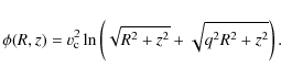
It generates, within the plane of symmetry z=0, a constant circular velocity curve of amplitude
Figures 1, 2 show the isodensity and isopotential contours for some values of q. The axis ratio of isodensity contours is q3/2 and for the isopotentials it is (1+q)/2, never less than 1/2. It can be shown (Toomre 1982) that any scale-free potential at the spherical limit (obtained here with q=1) is the potential of the singular isothermal sphere, while the flat disk limit (q=0) is the Mestel flat disk. With q >1, the Eq. (1) potential is prolate and at the limit
3 Velocity ellipsoid tilt
Since the Eq. (1) potential is scale-free we simply need to
determine the velocity ellipsoid orientation versus z at some given
radius R. We build the velocity ellipsoid numerically from orbit
integrations (
![]() orbits with
orbits with
![]() at
z=0). The velocity ellipsoid orientation for these distribution
functions is shown (Fig. 3), for R=1, versus z within
the meridional plane for potentials with flattenings q=0.3, 0.7.
Other approaches could be tried: see for instance, the analysis by
Evans et al. (1997) from the Jeans equations for scale-free
potentials with a flat rotation curve by applying an approximate third
integral (see also for scale-free potentials: Qian et al.
1995; Evans & de Zeeuw 1992; Qian 1992;
Hunter et al. 1984; de Zeeuw et al. 1996; Evans et al. 1997).
at
z=0). The velocity ellipsoid orientation for these distribution
functions is shown (Fig. 3), for R=1, versus z within
the meridional plane for potentials with flattenings q=0.3, 0.7.
Other approaches could be tried: see for instance, the analysis by
Evans et al. (1997) from the Jeans equations for scale-free
potentials with a flat rotation curve by applying an approximate third
integral (see also for scale-free potentials: Qian et al.
1995; Evans & de Zeeuw 1992; Qian 1992;
Hunter et al. 1984; de Zeeuw et al. 1996; Evans et al. 1997).
| |
Figure 1: Contours of isopotentials with q=0.8 and 0.2. |
| Open with DEXTER | |
| |
Figure 2: Contours of isodensities with q=0.8 and 0.2. |
| Open with DEXTER | |
Figure 4 shows the variation in the tilt angle ![]() at
R=8 and z=1 above the mid-plane versus the coefficient q.
at
R=8 and z=1 above the mid-plane versus the coefficient q.
![]() varies by 5 degrees from 2.2 to 7.1 degrees depending on
whether the density distribution is flat or spherical. This may be
compared with the recent determination by Siebert et al. (2008)
of the inclination of the velocity ellipsoid at 1 kpc below the
Galactic plane. From RAVE data (Zwitter et al. 2008), they
find an inclination
varies by 5 degrees from 2.2 to 7.1 degrees depending on
whether the density distribution is flat or spherical. This may be
compared with the recent determination by Siebert et al. (2008)
of the inclination of the velocity ellipsoid at 1 kpc below the
Galactic plane. From RAVE data (Zwitter et al. 2008), they
find an inclination
![]() degrees towards the Galactic
plane. They show it implies a moderate flattening of the dark halo by
exploring the velocity ellipsoid tilt within various galactic
potentials (Dehnen & Binney 1998). Within the potential of
the Besançon galactic model (Robin et al. 2003) (probably
the best current Galactic baryonic mass model) that includes a
spherical dark halo, we also determine the velocity ellispoid tilt
from numerical orbit integration and obtain
degrees towards the Galactic
plane. They show it implies a moderate flattening of the dark halo by
exploring the velocity ellipsoid tilt within various galactic
potentials (Dehnen & Binney 1998). Within the potential of
the Besançon galactic model (Robin et al. 2003) (probably
the best current Galactic baryonic mass model) that includes a
spherical dark halo, we also determine the velocity ellispoid tilt
from numerical orbit integration and obtain
![]() degrees
(Bienaymé et al. 2009). To summarize, within a spherical
Galactic potential, the tilt at 1 kpc above the plane at the solar
radius is about 7 degrees, and an extreme flattening of the dark
matter component is excluded, since the tilt would be close to 2 or 3
degrees (Fig. 4).
degrees
(Bienaymé et al. 2009). To summarize, within a spherical
Galactic potential, the tilt at 1 kpc above the plane at the solar
radius is about 7 degrees, and an extreme flattening of the dark
matter component is excluded, since the tilt would be close to 2 or 3
degrees (Fig. 4).
4 Other potential-density pairs
The Mestel disk potential can be generalized by introducing a core radius
a. It gives (Evans & Collett 1993; and quoted references
Rybicki 1974; and Zang 1976)

with the resulting surface density

and the rotation curve

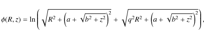
We generalize these Mestel disks with a core by applying the Miyamoto & Nagai (1975) method to generalize the Plummer spheroid and Kuzmin disk (see also Baes 2009). Thus we define the potential
It can be verified that this potential generates a positive spheroidal density distribution. With b=0 it may generate both a flat disk and a spheroid. The sum (a+b) constrains the size of the core, and bthe thickness of the disky part of the spheroid.
| |
Figure 3:
Vertical tilt of the velocity ellipsoid |
| Open with DEXTER | |
![\begin{figure}
\par\resizebox{8cm}{!}{
\includegraphics[angle=-90,width=8cm,clip]{9404fg4.ps}}
\end{figure}](/articles/aa/full_html/2009/23/aa09404-08/img17.png) |
Figure 4: Velocity ellipsoid inclination in degrees versus potential flattening q at R=8 and z=1. Dotted line: the expected inclination from Sect. 5, crosses: numerical determinations from orbit integration. |
| Open with DEXTER | |
![\begin{figure}
\par\resizebox{17cm}{!}{
\includegraphics[angle=0,width=5.4cm,cli...
...ace*{5mm}
\includegraphics[angle=0,width=5.4cm,clip]{9404fg5c.eps}}
\end{figure}](/articles/aa/full_html/2009/23/aa09404-08/img18.png) |
Figure 5: Isolevels for the density distribution resulting from the potential given by Eq. (4) with (a,b,q)=(5, 2, 1.3), (5, 2, 0.7), (0, 5, 0.5) from left to right. |
| Open with DEXTER | |
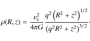
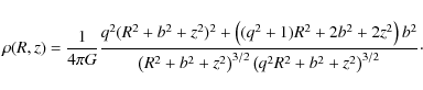
Potentials given by Eqs. (1) and (3) are peculiar cases (q=0 or a=b=0) of the more general potential
and the corresponding density is (if ![]() )
)
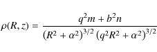
with
| (6) |
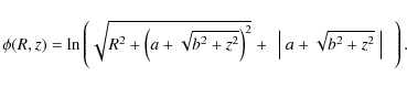
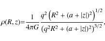
If a=0, it may be shortly written as
 |
(7) |
When b=0 and
 |
(8) |
 |
(9) |
With q=1, this is the potential-density pair defined by Brada & Milgrom (1995).
More generally, we obtain a spheroid potential producing a rising velocity curve, flat at large radii, the core radius depending only on q and on a+b. The parameter q modifies the flattening at large R and b the thickness of the disky part of the density distribution.
Thus, this generalization introduces a new family of potential-density pairs with general properties similar to the Miyamoto & Nagai potentials, but with flat circular velocity curves at large radii. Figures 5 illustrate isodensity contours for three such potentials. To conclude, we recall another three-parameter family of potential-density pairs obtained by Zhao (1996).
5 Anaytical estimate of the vertical velocity ellipsoid tilt
We examine the reliability of the Cuddeford & Amendt formulae (1991, Eqs. (90), (91) and (E10)) and Amendt & Cuddeford (1991, Eq. (104)) that predict the vertical tilt of the velocity ellipsoid within an axisymmetric potential, and we propose another formula that is more accurate at greater distances from the plane of symmetry z=0. For various potentials, we compare the expected tilt from these two expressions with the tilt obtained from numerical orbit integrations.
Cuddeford & Amendt (1991) analyze the consecutive moments of
the Boltzmann equation up to the 4th order by expanding these moments
in Taylor series assuming that
![]() is
small. Combining these moment equations, they derive expressions for
the velocity moments and obtain an approximate expression for the
tilt angle,
is
small. Combining these moment equations, they derive expressions for
the velocity moments and obtain an approximate expression for the
tilt angle,
![]() ,
which only depends on the
gravitational potential. They show that their expression is exact in
the case of axisymmetric Stäckel potentials, peculiar potentials
for which the tilt only depends on the potentials but not on the
exact distribution function. According to their initial hypothesis,
the formula must be generally valid when the considered distribution
of stellar orbits covers a sufficiently small domain (expecting that
the covered domain can be approximated with a Stäckel potential).
This should be the case of nearly circular orbits with small vertical
or radial oscillations.
,
which only depends on the
gravitational potential. They show that their expression is exact in
the case of axisymmetric Stäckel potentials, peculiar potentials
for which the tilt only depends on the potentials but not on the
exact distribution function. According to their initial hypothesis,
the formula must be generally valid when the considered distribution
of stellar orbits covers a sufficiently small domain (expecting that
the covered domain can be approximated with a Stäckel potential).
This should be the case of nearly circular orbits with small vertical
or radial oscillations.
The simplicity of the result obtained by Cuddeford & Amendt (1991) makes it extremely attractive. For instance Vallenari et al. (2006) use it to improve their recent galactic model of star counts and kinematics, which is dynamically self-consistent locally.
Inspired by their work, we propose a more direct expression derivated
from the generic equation (Ollongren 1962, Eq. (7.2)) that
defines axisymmetric Stäckel potentials:
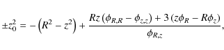
with a positive sign for prolate spheroidal coordinates, and a negative one for oblate ones (see de Zeeuw 1985, for a detailed description).
For a given potential ![]() ,
we substitute z0 from Eq. (10) in
the expression for the velocity ellipsoid tilt
,
we substitute z0 from Eq. (10) in
the expression for the velocity ellipsoid tilt ![]() given by Hori
& Liu (1963), which is exact in the case of Stäckel
potentials:
given by Hori
& Liu (1963), which is exact in the case of Stäckel
potentials:
Combining Eqs. (10) and (11) gives an estimate of the velocity ellipsoid inclination within axisymmetric potentials. We note that the Amendt & Cuddeford (1991) formula could have been obtained in the same way, just by differentiating the Ollongren equation with respect to z and replacing it within Eq. (11).
A noticeable difference between their expression and ours is that their formula is defined at z=0 and is exact for the Stäckel potential only at z=0, while our expression remains exact (for Stäckel potentials) at any z. This may be why our formula is in better agreement with the results of the numerical explorations described below.
Now, to verify the reliability of the estimated tilt angle ![]() given by Eqs. (10), (11), and the one given by Amendt &
Cuddeford (1991) formulae, we measure the tilt numerically
within a series of potentials. For this purpose, we build stationary
distribution functions with a library of
given by Eqs. (10), (11), and the one given by Amendt &
Cuddeford (1991) formulae, we measure the tilt numerically
within a series of potentials. For this purpose, we build stationary
distribution functions with a library of
![]() orbits for each
model using a 7th-order Runge-Kutta (Fehlberg 1968) with a
relative accuracy
orbits for each
model using a 7th-order Runge-Kutta (Fehlberg 1968) with a
relative accuracy
![]() .
Each orbit is integrated for
80 rotations, the initial conditions being drawn from a Shu
distribution function (we also tried a Dehnen disk distribution
function) with
.
Each orbit is integrated for
80 rotations, the initial conditions being drawn from a Shu
distribution function (we also tried a Dehnen disk distribution
function) with
![]() and
and
![]() (we also consider the 0.2-0.1 and 0.6-0.3 pairs). One
point is selected per orbit in the last 40 rotations.
(we also consider the 0.2-0.1 and 0.6-0.3 pairs). One
point is selected per orbit in the last 40 rotations.
Figures 6 show the inclination ![]() versus the distance
z from the plane of symmetry in the case of the Brada & Milgrom
(1995) disk+halo potential with a core radius a=3. The
tilt
versus the distance
z from the plane of symmetry in the case of the Brada & Milgrom
(1995) disk+halo potential with a core radius a=3. The
tilt ![]() is plotted versus z at four different galactic radii
R=1.5, 4.5, 7.5, and 10.5. The dark line is the analytical
estimate from Eqs. (10), (11), while the red line is the
result of numerical orbit integrations. The agreement between
numerical measures and the analytical estimate is satisfying in the
range of considered positions R and z. The estimated vertical
tilt is also shown in Fig. 4: at position R=8 and
z=1,
is plotted versus z at four different galactic radii
R=1.5, 4.5, 7.5, and 10.5. The dark line is the analytical
estimate from Eqs. (10), (11), while the red line is the
result of numerical orbit integrations. The agreement between
numerical measures and the analytical estimate is satisfying in the
range of considered positions R and z. The estimated vertical
tilt is also shown in Fig. 4: at position R=8 and
z=1, ![]() is plotted versus the flattening q of the
Eq. (1) potential. The agreement is satisfying for q between 0 and 1.
is plotted versus the flattening q of the
Eq. (1) potential. The agreement is satisfying for q between 0 and 1.
![\begin{figure}
\par\includegraphics[angle=270,width=4.3cm,clip]{9404fg6a.ps}\hsp...
...ace*{3mm}
\includegraphics[angle=270,width=4.3cm,clip]{9404fg6d.ps}
\end{figure}](/articles/aa/full_html/2009/23/aa09404-08/img38.png) |
Figure 6: Velocity ellipsoid tilt angles in degrees versus z within the Brada & Milgrom (1995) Disk+Halo potential at four galactic radii R=1.5, 4.5, 7.5 and 10.5 (from top left to bottom right). Red irregular line: numerical determination. Dark continuous line: analytical estimate. Dotted line: tilt within a spherical potential. |
| Open with DEXTER | |
We explored other potentials: a Kuzmin disk (a Stäckel potential to test our numerical process), the Mestel disk, the Brada & Milgrom potential, a logarithmic flattened potential, combined Kuzmin+logarithmic halo potentials. For these potentials our analytical estimate give excellent results in agreement with numerical determinations at a precision better than 1 degree at z/R=0.15.
With the slightly flattened spherical logarithmic potentials, the Amendt & Cuddeford (1991) formula is also an excellent estimate for the tilt (1 percent difference at z/R=0.15 with a potential axis ratio q=0.9). However, with the Mestel potential, it fails at any z (a null tilt is predicted), while it works correctly with the Brada and Milgrom potential, but only at radius close to or smaller than the core radius.
In conclusion, our analytical estimate of the vertical tilt of the
stellar velocity ellipsoid is accurate for various potentials and
vertical distances less than 0.15R. It also shows that at 1 kpc
above the Galactic plane at the solar radius, ![]() varies by 5 degrees depending on whether the potential is spherical or the dark
matter component is flat.
varies by 5 degrees depending on whether the potential is spherical or the dark
matter component is flat.
However, for an exponential disk, this estimate fails in the range R<2 or >4, in units of the scale length. The situation is similar for the potential given by Eq. (1) for ``flattening'' of q=2and neighboring values. An explanation for this deficiency is that the denominator of the r.h.s. of Eq. (11) is zero. In that case, the resulting value for z0 varies strongly with R or z. Since Eq. (10) is not a Stäckel fit, its domain of validity is determined by the condition that the estimate for z0 from Eq. (11) does not vary strongly over the considered (R,z)-domain. For deviations from this limit, more sophisticated methods of fitting potentials with Stäckel potentials are required (see for instance de Bruyne et al. 2000) to obtain more reliable estimates of the vertical tilt angle.
References
- Amendt, P., & Cuddeford, P. 1991, ApJ, 368, 79 [NASA ADS] [CrossRef] (In the text)
- Baes, M. 2009, MNRAS, 392, 1503 [NASA ADS] [CrossRef] (In the text)
- Bienaymé, O., Famaey, B., Wu, X., Zhao, H. S., & Aubert, D. 2009, A&A, 500, 801 [CrossRef] [EDP Sciences] (In the text)
- Binney, J., & Spergel, D. 1983, The nearby stars and the stellar luminosity, ed. A.G.D. Philip, & U. Schenectady (N.Y.: Davis Press), IAU Col., 76, 259 (In the text)
- Brada, R., & Milgrom, M. 1995, MNRAS, 276, 453 [NASA ADS] (In the text)
- Cuddeford, P., & Amendt, P. 1991, MNRAS, 253, 427 [NASA ADS] (In the text)
- Chereul, E., Crézé, M., & Bienaymé, O. 1998, A&A, 340, 384 [NASA ADS] (In the text)
- de Bruyne, V., Leeuwin, F., & Dejonghe, H. 2000, MNRAS, 311, 297 [NASA ADS] [CrossRef] (In the text)
- Dehnen, W., & Binney, J. 1998, MNRAS, 294, 429 [NASA ADS] [CrossRef] (In the text)
- de Zeeuw, P. T. 1985, MNRAS, 216, 273 [NASA ADS] (In the text)
- de Zeeuw, P. T., Evans, N. W., & Schwarzschild, M. 1996, MNRAS, 280, 903 [NASA ADS] (In the text)
- Evans, N. W., & Collett, J. L. 1993, MNRAS, 264 353 (In the text)
- Evans, N. W., & de Zeeuw, P. T. 1992, MNRAS, 257, 152 [NASA ADS] (In the text)
- Evans, N. W., van Häfner, R. M., & de Zeeuw, P. T. 1997, MNRAS, 286, 315 [NASA ADS] (In the text)
- Fehlberg E. 1968, NASA Technical Report, R-287 (In the text)
- Hori, L., & Liu, T. 1963, PASJ, 15, 100 [NASA ADS] (In the text)
- Hunter, J. H., Ball, R., & Gottesman, S. T. 1984, MNRAS, 208, 1 [NASA ADS] (In the text)
- Kent, S., & de Zeew, T. 1991, AJ, 102, 1994 [NASA ADS] [CrossRef] (In the text)
- Kuijken, K., & Gilmore, G. 1989, MNRAS, 239, 571 [NASA ADS] (In the text)
- Miyamoto, M., & Nagai, R. 1975, PASJ, 27, 533 [NASA ADS] (In the text)
- Ollongren, A. 1962, B.A.N., 16, 241 [NASA ADS] (In the text)
- Qian, E. 1992, MNRAS, 257, 581 [NASA ADS] (In the text)
- Qian, E., de Zeeuw, P. T., van der Marel, R. P., & Hunter, C. 1995, MNRAS, 274, 602 [NASA ADS] (In the text)
- Robin, A. C., Reylé, C., Derrière, S., & Picaud, S. 2003, A&A, 409, 523 [NASA ADS] [CrossRef] [EDP Sciences] (In the text)
- Shapiro, K., Gerssen, J., & van der Marel, R. 2003, ApJ, 126, 2707 [NASA ADS] (In the text)
- Siebert, A., Bienaymé, O., Binney, J., et al. 2008, MNRAS, 391, 793 [NASA ADS] [CrossRef] (In the text)
- Soubiran, C., Bienaymé, O., Mishenina, T. V., & Kovtyukh, V. V. 2008, A&A, 480, 91 [NASA ADS] [CrossRef] [EDP Sciences] (In the text)
- Toomre, A. 1982, ApJ, 259, 535 [NASA ADS] [CrossRef] (In the text)
- Vallenari, A., Pasetto, S., Bertelli, G., et al. 2006, A&A, 451, 125 [NASA ADS] [CrossRef] [EDP Sciences]
- Zang, T. A. 1976, Ph.D. Thesis, Massachusetts Institute of Technology (In the text)
- Zhao, H. S. 1996, MNRAS, 278, 488 [NASA ADS] (In the text)
- Zwitter, T., Siebert, A., Munari, U., et al. 2008, AJ, 136, 421 [NASA ADS] [CrossRef] (In the text)
All Figures
| |
Figure 1: Contours of isopotentials with q=0.8 and 0.2. |
| Open with DEXTER | |
| In the text | |
| |
Figure 2: Contours of isodensities with q=0.8 and 0.2. |
| Open with DEXTER | |
| In the text | |
| |
Figure 3:
Vertical tilt of the velocity ellipsoid |
| Open with DEXTER | |
| In the text | |
| |
Figure 4: Velocity ellipsoid inclination in degrees versus potential flattening q at R=8 and z=1. Dotted line: the expected inclination from Sect. 5, crosses: numerical determinations from orbit integration. |
| Open with DEXTER | |
| In the text | |
| |
Figure 5: Isolevels for the density distribution resulting from the potential given by Eq. (4) with (a,b,q)=(5, 2, 1.3), (5, 2, 0.7), (0, 5, 0.5) from left to right. |
| Open with DEXTER | |
| In the text | |
| |
Figure 6: Velocity ellipsoid tilt angles in degrees versus z within the Brada & Milgrom (1995) Disk+Halo potential at four galactic radii R=1.5, 4.5, 7.5 and 10.5 (from top left to bottom right). Red irregular line: numerical determination. Dark continuous line: analytical estimate. Dotted line: tilt within a spherical potential. |
| Open with DEXTER | |
| In the text | |
Copyright ESO 2009
Current usage metrics show cumulative count of Article Views (full-text article views including HTML views, PDF and ePub downloads, according to the available data) and Abstracts Views on Vision4Press platform.
Data correspond to usage on the plateform after 2015. The current usage metrics is available 48-96 hours after online publication and is updated daily on week days.
Initial download of the metrics may take a while.