| Issue |
A&A
Volume 499, Number 3, June I 2009
|
|
|---|---|---|
| Page(s) | 711 - 722 | |
| Section | Extragalactic astronomy | |
| DOI | https://doi.org/10.1051/0004-6361/200811472 | |
| Published online | 27 March 2009 | |
The chemical evolution of galaxies within the IGIMF theory:
the [ /Fe] ratios and downsizing
S. Recchi1,2 - F. Calura3 - P. Kroupa4
1 - Institute of Astronomy, Vienna University,
Türkenschanzstrasse 17, 1180 Vienna, Austria
2 -
INAF - Osservatorio Astronomico di Trieste,
via G.B. Tiepolo 11, 34143 Trieste, Italy
3 -
Astronomy Department, Trieste University,
via G.B. Tiepolo 11, 34143 Trieste, Italy
4 -
Argelander Institute for Astronomy, Bonn University,
Auf dem Hügel 71, 53121 Bonn, Germany
Received 4 December 2008 / Accepted 9 March 2009
Abstract
Context. The chemical evolution of galaxies is investigated within the framework of the star formation rate (SFR) dependent integrated galactic initial mass function (IGIMF).
Aims. We study how the global chemical evolution of a galaxy and in particular how [![]() /Fe] abundance ratios are affected by the predicted steepening of the IGIMF with decreasing SFR.
/Fe] abundance ratios are affected by the predicted steepening of the IGIMF with decreasing SFR.
Methods. We use analytical and semi-analytical calculations to evaluate the mass-weighted and luminosity-weighted [![]() /Fe] ratios in early-type galaxies of different masses.
/Fe] ratios in early-type galaxies of different masses.
Results. The models with variable IGIMF produce an [![]() /Fe] vs. velocity dispersion relation which has the same slope as the observations of massive galaxies, irrespective of the model parameters, provided that the star formation duration inversely correlates with the mass of the galaxy (downsizing). These models also produce steeper [
/Fe] vs. velocity dispersion relation which has the same slope as the observations of massive galaxies, irrespective of the model parameters, provided that the star formation duration inversely correlates with the mass of the galaxy (downsizing). These models also produce steeper [![]() /Fe] vs.
/Fe] vs. ![]() relations in low-mass early-type galaxies and this trend is consistent with the observations. Constant IMF models are able to reproduce the [
relations in low-mass early-type galaxies and this trend is consistent with the observations. Constant IMF models are able to reproduce the [![]() /Fe] ratios in large elliptical galaxies as well, but they do not predict this change of slope for small galaxies. In order to obtain the best fit between our results and observations, the downsizing effect (i.e. the shorter duration of the star formation in larger galaxies) must be milder than previously thought.
/Fe] ratios in large elliptical galaxies as well, but they do not predict this change of slope for small galaxies. In order to obtain the best fit between our results and observations, the downsizing effect (i.e. the shorter duration of the star formation in larger galaxies) must be milder than previously thought.
Key words: stars: abundances - supernovae: general - galaxies: evolution - galaxies: elliptical and lenticular, cD - galaxies: star clusters
1 Introduction
It is nowadays widely accepted that most stars in galaxies form in star
clusters (Tutukov 1978; Lada & Lada 2003). This has been
observed in a number of different galaxies, from the Milky Way to the dwarf
galaxies of the Local Group (Wyse et al. 2002; Massey 2003;
Piskunov et al. 2004). Within each star cluster, the initial mass
function (IMF) can be well approximated by the canonical two-part power-law
form
![]() (e.g. Pflamm-Altenburg et al.
2007, hereafter PWK07). Massey & Hunter (1998) have shown
that for stellar masses m> a few
(e.g. Pflamm-Altenburg et al.
2007, hereafter PWK07). Massey & Hunter (1998) have shown
that for stellar masses m> a few ![]() a slope similar to the Salpeter (1955) index (i.e.
a slope similar to the Salpeter (1955) index (i.e.
![]() )
can approximate well the IMF in
clusters and OB associations for a wide range of metallicities, whereas many
studies have shown that the IMF flattens out below
)
can approximate well the IMF in
clusters and OB associations for a wide range of metallicities, whereas many
studies have shown that the IMF flattens out below
![]() (Kroupa et al. 1993; Chabrier 2001).
(Kroupa et al. 1993; Chabrier 2001).
On the other hand, star clusters are also apparently distributed according to
a single-slope power law,
![]() ,
where
,
where
![]() is the stellar mass of the embedded star cluster. There is a
general consensus that this slope
is the stellar mass of the embedded star cluster. There is a
general consensus that this slope ![]() should be of the order of
should be of the order of ![]() 2
(Zhang & Fall 1999; Lada & Lada 2003; Hunter et al. 2003), although a
2
(Zhang & Fall 1999; Lada & Lada 2003; Hunter et al. 2003), although a ![]() as high as 2.4 can also be realistic
(Weidner et al. 2004). According to this correlation,
small embedded clusters are more numerous in galaxies. They provide therefore
most of the stars but not most of the massive ones, since these are
preferentially formed in massive clusters (Weidner & Kroupa 2006). As
a consequence of this mass distribution of embedded clusters, the integrated
IMF in galaxies, the IGIMF, can be steeper than the stellar IMF within each
single star cluster (Kroupa & Weidner 2003; Weidner & Kroupa 2005).
as high as 2.4 can also be realistic
(Weidner et al. 2004). According to this correlation,
small embedded clusters are more numerous in galaxies. They provide therefore
most of the stars but not most of the massive ones, since these are
preferentially formed in massive clusters (Weidner & Kroupa 2006). As
a consequence of this mass distribution of embedded clusters, the integrated
IMF in galaxies, the IGIMF, can be steeper than the stellar IMF within each
single star cluster (Kroupa & Weidner 2003; Weidner & Kroupa 2005).
The Salpeter IMF slope has been used in a very wide range of modelling,
providing good fits with observations concerning the cosmic star formation
history (Calura et al. 2004), the X-ray properties of
elliptical galaxies (Pipino et al. 2005), the chemical evolution of
dwarf galaxies (Larsen et al. 2001) and of the Milky
Way (Pilyugin & Edmunds 1996; but see also Romano et al. 2005). Broadly speaking, a flatter than Salpeter IMF produces a
larger fraction of massive stars. The high level of production of oxygen (and
of ![]() -elements in general) leads to lower [Z/O] metallicity ratios. A
steep IMF slope would instead be biased towards low- and intermediate-mass
stars, underproducing oxygen and therefore resulting in larger [N/O] and [C/O]
abundance ratios. On the other hand, iron will also be overproduced compared
to
-elements in general) leads to lower [Z/O] metallicity ratios. A
steep IMF slope would instead be biased towards low- and intermediate-mass
stars, underproducing oxygen and therefore resulting in larger [N/O] and [C/O]
abundance ratios. On the other hand, iron will also be overproduced compared
to ![]() -elements, since it comes mainly from type Ia SNe which originate
from C-O deflagration of binary systems of intermediate mass. Therefore,
galaxies characterized by a steep IMF will tend to have [
-elements, since it comes mainly from type Ia SNe which originate
from C-O deflagration of binary systems of intermediate mass. Therefore,
galaxies characterized by a steep IMF will tend to have [![]() /Fe] ratios
lower than models in which the IMF is flat.
/Fe] ratios
lower than models in which the IMF is flat.
The scenario of a variable integrated galactic initial mass function (IGIMF)
has been applied in models of chemical evolution (Köppen et al. 2007), producing an excellent agreement with the mass-metallicity
relation found by Tremonti et al. (2004). However, these authors
consider only the effect of the IGIMF on the global metallicity and the
evolution of abundance ratios has not yet been explored in the literature. In
a series of papers we plan to study the impact of the IGIMF on the abundance
ratios in different classes of galaxies, using different methodologies. In
this paper we study, by means of simple analytical and semi-analytical models,
the evolution of [![]() /Fe] ratios in galaxies, in particular in early-type
ones. It is now well established that the [
/Fe] ratios in galaxies, in particular in early-type
ones. It is now well established that the [![]() /Fe] ratios in the cores
of elliptical galaxies increase with galactic mass (Weiss et al. 1995; Kuntschner et al. 2001) and this poses
serious problems to the current paradigm of hierarchical build-up of galaxies
(see e.g. Thomas et al. 2005, hereafter THOM05; Nagashima et al. 2005; Pipino et al. 2009; Calura & Menci, in
preparation). In fact, in the classical hierarchical models the most massive
ellipticals take a longer time to assemble and therefore form stars for a
longer time than less massive galaxies, thus producing a a trend of
[
/Fe] ratios in the cores
of elliptical galaxies increase with galactic mass (Weiss et al. 1995; Kuntschner et al. 2001) and this poses
serious problems to the current paradigm of hierarchical build-up of galaxies
(see e.g. Thomas et al. 2005, hereafter THOM05; Nagashima et al. 2005; Pipino et al. 2009; Calura & Menci, in
preparation). In fact, in the classical hierarchical models the most massive
ellipticals take a longer time to assemble and therefore form stars for a
longer time than less massive galaxies, thus producing a a trend of
[![]() /Fe] vs. mass which is opposite to what is observed (see Thomas et al. 2002; Matteucci 2007).
/Fe] vs. mass which is opposite to what is observed (see Thomas et al. 2002; Matteucci 2007).
We will show in this paper that the trend of increasing [![]() /Fe]
vs. galaxy mass is naturally accounted for in models of elliptical galaxies in
which the IGIMF is implemented. The second paper of this series will be
devoted to the study of the chemical evolution of the Solar Neighborhood and
of the local dwarf galaxies and in this case we will make use of detailed
chemical evolution models. Another paper of this series will study the
evolution of galaxies by means of chemodynamical models, in order to analyze
how the IGIMF changes the feedback of the ongoing star formation in galaxies
and how this affects the chemical evolution.
/Fe]
vs. galaxy mass is naturally accounted for in models of elliptical galaxies in
which the IGIMF is implemented. The second paper of this series will be
devoted to the study of the chemical evolution of the Solar Neighborhood and
of the local dwarf galaxies and in this case we will make use of detailed
chemical evolution models. Another paper of this series will study the
evolution of galaxies by means of chemodynamical models, in order to analyze
how the IGIMF changes the feedback of the ongoing star formation in galaxies
and how this affects the chemical evolution.
The plan of the present paper is as follows. In Sect. 2 we summarize the IGIMF
theory and the formulations we adopt. In Sect. 3 we describe how we calculate
the type Ia and type II SN rates in galaxies in which the SFR is given. Once
we know the type Ia and type II SN rates, it is possible to calculate the
[![]() /Fe] ratios. This has been done in Sect. 4 for ellipticals and
early-type galaxies in general. A discussion and the main conclusions are
presented in Sect. 5.
/Fe] ratios. This has been done in Sect. 4 for ellipticals and
early-type galaxies in general. A discussion and the main conclusions are
presented in Sect. 5.
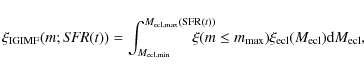
2 The determination of the integrated galactic initial mass function
The determination of the IGIMF has been described previously (Kroupa &
Weidner 2003; Weidner & Kroupa 2005; PWK07). The IGIMF theory
is based on the assumption that all the stars in a galaxy form in star
clusters. Surveys of star-formation in the local Milky Way disk have shown
that 70 to 90% of all stars appear to form in embedded clusters (Lada &
Lada 2003; Evans et al. 2009). The remaining 10-30% of the
apparently distributed population may stem from a large number of short-lived
small clusters that evolve rapidly by dissolving through energy equipartition
and residual gas expulsion. It is therefore reasonable to assume that star
formation occurs in embedded clusters with masses ranging from a few ![]() upwards. The IGIMF, integrated over the whole population of embedded clusters
forming in a galaxy, becomes
upwards. The IGIMF, integrated over the whole population of embedded clusters
forming in a galaxy, becomes
 |
(1) |
where
where
The stellar IMF (i.e. the IMF within each embedded cluster) has the canonical
form
![]() ,
with
,
with
![]() for 0.08
for 0.08
![]()
![]() and
and
![]() (i.e. the Salpeter slope) for
(i.e. the Salpeter slope) for
![]()
![]() ,
where
,
where
![]() depends on the mass of
the embedded cluster. In order to determine
depends on the mass of
the embedded cluster. In order to determine
![]() and the
proportionality constant k we have to solve the following two equations
(Kroupa & Weidner 2003):
and the
proportionality constant k we have to solve the following two equations
(Kroupa & Weidner 2003):
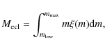
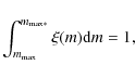
where
The last ingredient we need is the distribution function of embedded clusters,
![]() ,
which, as we have mentioned in the
Introduction, we can assume proportional to
,
which, as we have mentioned in the
Introduction, we can assume proportional to
![]() .
In this
work we have assumed 3 possible values of
.
In this
work we have assumed 3 possible values of ![]() :
1.00 (model BETA100), 2.00
(model BETA200) and 2.35 (model BETA235). In Fig. 1 we have
plotted the resulting IGIMFs for different values of the SFR. In particular,
we have tested 20 SFRs, ranging from 10-4 to
:
1.00 (model BETA100), 2.00
(model BETA200) and 2.35 (model BETA235). In Fig. 1 we have
plotted the resulting IGIMFs for different values of the SFR. In particular,
we have tested 20 SFRs, ranging from 10-4 to
![]() yr-1,
equally spaced in logarithm. To appreciate better the differences between
various models, we have plotted in Fig. 2 IGIMFs for 3 different values of the SFR:
yr-1,
equally spaced in logarithm. To appreciate better the differences between
various models, we have plotted in Fig. 2 IGIMFs for 3 different values of the SFR:
![]() yr-1 (heavy
lines),
yr-1 (heavy
lines),
![]() yr-1 (middle lines),
yr-1 (middle lines),
![]() yr-1 (light lines). We have considered all the
possible values of
yr-1 (light lines). We have considered all the
possible values of ![]() :
model BETA100 (dashed lines), BETA200 (dotted
lines), BETA235 (solid lines). For clarity, we have plotted the IGIMFs only
for masses larger than
:
model BETA100 (dashed lines), BETA200 (dotted
lines), BETA235 (solid lines). For clarity, we have plotted the IGIMFs only
for masses larger than ![]() 2
2 ![]() ,
since in the range of low mass
stars the IGIMFs do not vary. As expected, the model with the steepest
distribution of embedded clusters (model BETA235) produces also the steepest
IGIMFs. This is due to the fact that model BETA235 is biased towards embedded
clusters of low mass, therefore the probability of finding high mass stars in
this cluster population is lower.
,
since in the range of low mass
stars the IGIMFs do not vary. As expected, the model with the steepest
distribution of embedded clusters (model BETA235) produces also the steepest
IGIMFs. This is due to the fact that model BETA235 is biased towards embedded
clusters of low mass, therefore the probability of finding high mass stars in
this cluster population is lower.
![\begin{figure}
\par\includegraphics[width=8.5cm,clip]{1472fig1.eps}
\end{figure}](/articles/aa/full_html/2009/21/aa11472-08/img60.png) |
Figure 1:
IGIMFs for different distributions of embedded
clusters (e.g. different values of |
| Open with DEXTER | |
![\begin{figure}
\par\includegraphics[width=8.5cm,clip]{1472fig2.eps}
\end{figure}](/articles/aa/full_html/2009/21/aa11472-08/img64.png) |
Figure 2:
IGIMFs for different SFRs: |
| Open with DEXTER | |
We can also notice from Fig. 2 that the differences between
IGIMFs with
![]() yr-1 (middle lines) and
yr-1 (middle lines) and
![]() yr-1 (light lines) are not very pronounced. This is
due to the fact that for both these SFRs, the maximum possible mass of the
embedded cluster is very high (see Eq. (2)), therefore in both
cases the upper possible stellar mass of the whole galaxy is very close to the
theoretical limit of
yr-1 (light lines) are not very pronounced. This is
due to the fact that for both these SFRs, the maximum possible mass of the
embedded cluster is very high (see Eq. (2)), therefore in both
cases the upper possible stellar mass of the whole galaxy is very close to the
theoretical limit of
![]() .
This can be seen in Fig. 3
(lower panel) in which we plot the variation of
.
This can be seen in Fig. 3
(lower panel) in which we plot the variation of
![]() as a function of
SFR as deduced from Eqs. (4) and (3). This
correlation is valid for all the possible values of
as a function of
SFR as deduced from Eqs. (4) and (3). This
correlation is valid for all the possible values of ![]() because it is
determined by
because it is
determined by ![]() and not by
and not by
![]() .
As we can
see from Figs. 1 and 2, the IGIMFs are
characterized by a nearly uniform decline, which follows approximately a power
law, and a sharp cutoff when m gets close to
.
As we can
see from Figs. 1 and 2, the IGIMFs are
characterized by a nearly uniform decline, which follows approximately a power
law, and a sharp cutoff when m gets close to
![]() .
In
Fig. 3 (upper panel) we therefore also plot the slope that better
approximates the IGIMF in the range 3-16
.
In
Fig. 3 (upper panel) we therefore also plot the slope that better
approximates the IGIMF in the range 3-16 ![]() .
This is the range of
masses where most of the progenitors of SNeII and SNeIa originate (see
Sect. 3). Of course, the steeper the distribution of embedded clusters, the
steeper the corresponding IGIMFs. Figure 3 shows also what we have
noticed before, namely that the various IGIMFs saturate for
.
This is the range of
masses where most of the progenitors of SNeII and SNeIa originate (see
Sect. 3). Of course, the steeper the distribution of embedded clusters, the
steeper the corresponding IGIMFs. Figure 3 shows also what we have
noticed before, namely that the various IGIMFs saturate for
![]() yr-1. Finally, in Fig. 3 (middle panel)
yr-1. Finally, in Fig. 3 (middle panel)
![]() is shown as a function of the SFR for the various models.
is shown as a function of the SFR for the various models.
![]() is the
number of stars per unit mass in one stellar generation (see e.g. Greggio 2005) and its value is given by
is the
number of stars per unit mass in one stellar generation (see e.g. Greggio 2005) and its value is given by
 |
(5) |
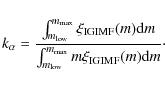
This parameter is useful to calculate the SNII rates (see Sect. 3).
![\begin{figure}
\par\includegraphics[width=8.5cm,clip]{1472fig3.eps}
\end{figure}](/articles/aa/full_html/2009/21/aa11472-08/img69.png) |
Figure 3:
Lower panel:
|
| Open with DEXTER | |
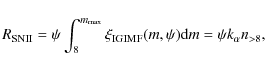
3 The determination of type Ia and type II SN rates
3.1 Type II SN rates
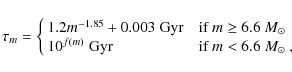
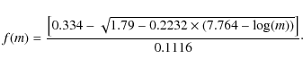
Stars in the range
![]() (where
(where
![]() is the
mass limit for the formation of a degenerate C-O core) are generally supposed
to end their lives as core-collapse SNe. These SNe are divided into
SNeII, SNeIb and SNeIc according to their spectra. For our purposes, this
distinction is not useful and we will suppose that all the core-collapse
supernovae are indeed SNeII. These SNe produce the bulk of
is the
mass limit for the formation of a degenerate C-O core) are generally supposed
to end their lives as core-collapse SNe. These SNe are divided into
SNeII, SNeIb and SNeIc according to their spectra. For our purposes, this
distinction is not useful and we will suppose that all the core-collapse
supernovae are indeed SNeII. These SNe produce the bulk of ![]() -elements
and some iron (one third approximately). The standard value of
-elements
and some iron (one third approximately). The standard value of
![]() is
is ![]() but stellar models with overshooting predict lower values
(e.g. Marigo 2001). However, stars more massive than
but stellar models with overshooting predict lower values
(e.g. Marigo 2001). However, stars more massive than
![]() can still develop a degenerate O-Ne core and end their lives as
electron-capture SNe (Siess 2007). We will assume for simplicity
that all the stars with masses larger than
can still develop a degenerate O-Ne core and end their lives as
electron-capture SNe (Siess 2007). We will assume for simplicity
that all the stars with masses larger than ![]() end their lives as
SNeII, therefore the SNII rate is simply given by the rate at which massive
stars die, namely:
end their lives as
SNeII, therefore the SNII rate is simply given by the rate at which massive
stars die, namely:
![\begin{displaymath}R_{\rm SNII} (t) = \int_8^{m_{\rm max}} \psi (t - \tau_m) \xi_{\rm IGIMF} [m, \psi
(t - \tau_m)] {\rm d}m,
\end{displaymath}](/articles/aa/full_html/2009/21/aa11472-08/img73.png)
where
 |
(7) |
where
 |
(8) |
In Eq. (6) the IGIMF is calculated by considering the SFR at the time
![\begin{figure}
\par\includegraphics[width=8.8cm,clip]{1472fig4.eps}
\end{figure}](/articles/aa/full_html/2009/21/aa11472-08/img78.png) |
Figure 4:
Lower panel:
|
| Open with DEXTER | |
![\begin{figure}
\par\includegraphics[width=8.5cm,clip]{1472fig5.eps}
\end{figure}](/articles/aa/full_html/2009/21/aa11472-08/img81.png) |
Figure 5:
|
| Open with DEXTER | |
It is instructive to analyze models in which SFR is constant during the whole
evolution of the galaxy. In this way, Eq. (6) simplifies into
where, as we have seen in Sect. 2,
It is nowadays popular to consider SN rates normalized to the stellar mass of
the considered galaxy. The usually chosen unit of measure is the SNuM (1 SNuM
= 1 SN cen-1
10-10 M*-1, where M* is the current stellar
mass of the galaxy). In this case, models in which the SFR is constant cannot
attain a constant Type II SN rate in SNuM since the stellar mass of the galaxy
increases with time. We therefore calculated
![]() in SNuM as a function
of time for the various models. The stellar mass of the galaxy at each time
t is given by
in SNuM as a function
of time for the various models. The stellar mass of the galaxy at each time
t is given by
![]() ,
where
f< m (t) is
the mass fraction of stars, born until the time t, that have not yet died.
,
where
f< m (t) is
the mass fraction of stars, born until the time t, that have not yet died.
Figure 5 shows the evolution with time of the Type II SN rate for different models and different SFRs, assuming a constant SFR for 14 Gyr. These results are compared with the average SNeII rates (in SNuM), observationally derived by Mannucci et al. (2005) in S0a/b galaxies (solid boxes), Sbc/d galaxies (dotted boxes) and irregular ones (dashed boxes). We can notice that, for the models BETA100 and BETA200 only the mildest SFRs can reproduce the final SNII rates in S0a/b galaxies, whereas model BETA235 can fit the final SNII rate of S0a/b galaxies for a wide range of SFRs. On the other hand, all the models predict final SNII rates significantly below the observations of irregular galaxies and the final values for model BETA235 fail also to fit the observed rates in Sbc/d galaxies. It is important to note, however, that the stellar mass in galaxies is usually calculated assuming some (constant) IMF. Under the assumption that the IMF changes with the SFR, the determinations of the stellar masses must be revisited. PWK07 showed that the IGIMF effect (i.e. the suppression of the number of massive stars with respect of low-mass stars) can be very significant in dwarf galaxies, whereas in large galaxies it tends to be very small. Moreover, a constant SFR for 14 Gyr is not a reasonable description of the star formation history of irregular (and Sbc/d) galaxies which often experience an increase of the SFR in the last Gyrs of their evolution (see e.g. Calura & Matteucci 2006). For this reason, the calculated SNII rates of late type galaxies tend to fit the observations at younger ages.
3.2 Type Ia SN rates
In order to calculate the SNIa rates, we assume the so-called Single
Degenerate Scenario of SNIa formation. It is commonly assumed that a SNIa
explodes when a C-O white dwarf in a binary system reaches the Chandrasekhar
mass after mass accretion from a companion star. According to the Single
Degenerate channel of SNIa explosion, the accretion of matter occurs via mass
transfer from a non-degenerate companion (a red giant or a main sequence star)
filling its Roche lobe (Whelan & Iben 1973). In this way, the SNIa
rate depends on the number distribution of C-O white dwarfs, but also on the
mass ratio between primary and secondary stars in a binary system. The SNIa
rate in the framework of the Single Degenerate Scenario has been calculated
analytically by a number of authors assuming a universal IMF (see Valiante 2009, and references therein). Here we follow the formulation of
Greggio & Renzini (1983) and Matteucci & Recchi (2001) but we
modify it to take into account that, in the framework of the IGIMF, the IMF
changes according to the SFR. The SNIa rate in this case turns out to be:
![$\displaystyle R_{\rm Ia} (t)= A \int_{m_{\rm B, inf}}^{m_{\rm B, sup}}
\int_{\m...
...\xi_{\rm IGIMF} [m_{\rm B}, \psi
(t - \tau_{m_2})]{\rm d}\mu~ {\rm d}m_{\rm B},$](/articles/aa/full_html/2009/21/aa11472-08/img86.png)
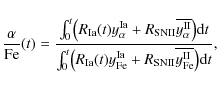
where A is a normalization constant (assumed to be 0.09 in the following). Although theoretical arguments demonstrate that A should be small (e.g. Maoz 2008) its value is usually calibrated with the Milky Way. Unfortunately, our analytical approach does not allow us to simulate the Milky Way within the IGIMF theory, therefore we take 0.09 as a reference value and postpone a more careful discussion about it to the follow-up numerical paper (but see also Sect. 4 for a study of the variation of A for early-type galaxies).
| (11) |
| (12) |
![\begin{displaymath}\mu_{\rm min} = {\rm max} \biggl[{m_2 (t) \over m_{\rm B}},
{{m_{\rm B} - 8~M_{\odot}}\over m_{\rm B}}\biggr]\cdot
\end{displaymath}](/articles/aa/full_html/2009/21/aa11472-08/img94.png) |
(13) |
The distribution function of mass ratios is generally described as a power law (
Figure 6 shows the evolution with time of the type Ia SN rate for
different models and different SFRs, analogously to Fig. 5 for
SNeII rates. Also shown (dashed lines) for comparison are SNIa rates obtained
for a model with fixed (i.e. not SFR-dependent) IMF. We assume the canonical
stellar IMF (i.e. the IMF within each embedded cluster) which, as mentioned in
Sect. 2, has the form
![]() ,
with
,
with
![]() for
for
![]() and
and
![]() above
above
![]() .
As we can see, at large SFRs model BETA100 produces rates almost
indistinguishable from the ones obtained with the fixed canonical IMF (see
also Kroupa & Weidner 2003). In this figure
.
As we can see, at large SFRs model BETA100 produces rates almost
indistinguishable from the ones obtained with the fixed canonical IMF (see
also Kroupa & Weidner 2003). In this figure ![]() is assumed to be
2 (Tutukov & Yungelson 1980). This large value of
is assumed to be
2 (Tutukov & Yungelson 1980). This large value of ![]() favors the
occurrence of SNeIa in binary systems with similar masses. Such a steep mass
ratio distribution that favors equal-mass binaries may result from dynamical
evolution of stellar populations in long-lived star clusters (Shara & Hurley
2002). We can notice again that only model BETA235 at very low SFRs
seems able to reproduce the SNIa rates in S0a/b and E/S0 galaxies. However,
we point out that the comparison with the observed SNIa rates in elliptical
galaxies is meaningless because they stopped forming stars several Gyr ago and
they have evolved passively since then. For them we cannot therefore assume a
constant SFR for 14 Gyr (see Sect. 4). On the other hand,
model BETA235 produces SNIa rates that only match the observed rates in dwarf
irregular galaxies at their peak. Therefore, assuming
favors the
occurrence of SNeIa in binary systems with similar masses. Such a steep mass
ratio distribution that favors equal-mass binaries may result from dynamical
evolution of stellar populations in long-lived star clusters (Shara & Hurley
2002). We can notice again that only model BETA235 at very low SFRs
seems able to reproduce the SNIa rates in S0a/b and E/S0 galaxies. However,
we point out that the comparison with the observed SNIa rates in elliptical
galaxies is meaningless because they stopped forming stars several Gyr ago and
they have evolved passively since then. For them we cannot therefore assume a
constant SFR for 14 Gyr (see Sect. 4). On the other hand,
model BETA235 produces SNIa rates that only match the observed rates in dwarf
irregular galaxies at their peak. Therefore, assuming
![]() ,
the best
value for
,
the best
value for ![]() seems to be 2 (but see the comment in Sect. 3.1
about the possible inconsistency of the published determination of stellar
masses, at least for irregular galaxies). To show the dependence of the
results on
seems to be 2 (but see the comment in Sect. 3.1
about the possible inconsistency of the published determination of stellar
masses, at least for irregular galaxies). To show the dependence of the
results on ![]() we show in Fig. 7 the SNeIa rates
obtained assuming
we show in Fig. 7 the SNeIa rates
obtained assuming
![]() .
This flatter distribution function implies
that a larger fraction of binary systems with small mass ratios end up as
SNeIa. We can notice from this figure that the observed SNIa rates in spiral
galaxies are reproduced by a larger range of SFRs, whereas the disagreement
with the observed rates in irregular galaxies worsens.
.
This flatter distribution function implies
that a larger fraction of binary systems with small mass ratios end up as
SNeIa. We can notice from this figure that the observed SNIa rates in spiral
galaxies are reproduced by a larger range of SFRs, whereas the disagreement
with the observed rates in irregular galaxies worsens.
![\begin{figure}
\par\includegraphics[width=8.5cm,clip]{1472fig6.eps}
\end{figure}](/articles/aa/full_html/2009/21/aa11472-08/img100.png) |
Figure 6:
|
| Open with DEXTER | |
![\begin{figure}
\par\includegraphics[width=8.5cm,clip]{1472fig7.eps}
\end{figure}](/articles/aa/full_html/2009/21/aa11472-08/img101.png) |
Figure 7:
As in Fig. 6 but for
|
| Open with DEXTER | |
4 A test of the IGIMF: [/Fe] ratios in early-type
galaxies
The study of the average stellar [![]() /Fe] ratio in galaxies represents an
important constraint for our models, since this quantity depends both on the
adopted galactic star formation history and on the stellar IMF (Matteucci 2001). In local ellipticals, the observed correlation between the
central velocity dispersion
/Fe] ratio in galaxies represents an
important constraint for our models, since this quantity depends both on the
adopted galactic star formation history and on the stellar IMF (Matteucci 2001). In local ellipticals, the observed correlation between the
central velocity dispersion ![]() ,
which reflects the total stellar mass,
and the stellar [
,
which reflects the total stellar mass,
and the stellar [![]() /Fe] is interpreted as due to the shorter star
formation timescales in the most massive galaxies (Pipino & Mattuecci
2004; THOM05) which in turn implies also that the most massive galaxies
experience the most intense episodes of star formation. For this reason, the
average stellar [
/Fe] is interpreted as due to the shorter star
formation timescales in the most massive galaxies (Pipino & Mattuecci
2004; THOM05) which in turn implies also that the most massive galaxies
experience the most intense episodes of star formation. For this reason, the
average stellar [![]() /Fe] vs.
/Fe] vs. ![]() relation represents a valuable test
for the IGIMF, since the IGIMF is a function of the galactic star formation
rate. The issue of a variable IMF among elliptical galaxies to explain the
[
relation represents a valuable test
for the IGIMF, since the IGIMF is a function of the galactic star formation
rate. The issue of a variable IMF among elliptical galaxies to explain the
[![]() /Fe] vs.
/Fe] vs. ![]() relation has already been explored with success by
Matteucci (1994) but assuming ad hoc variations of the IMF slope. In
this section we test, using well-established and observationally constrained
star formation histories of early-type galaxies of various masses, if the
physically motivated IGIMF can equally well reproduce this correlation.
relation has already been explored with success by
Matteucci (1994) but assuming ad hoc variations of the IMF slope. In
this section we test, using well-established and observationally constrained
star formation histories of early-type galaxies of various masses, if the
physically motivated IGIMF can equally well reproduce this correlation.
To simplify the calculations, the SFR is assumed to be constant over a period
of time ![]() .
We have numerically tested that this crude approximation
of the star formation history does not significantly affect the results. The
value of
.
We have numerically tested that this crude approximation
of the star formation history does not significantly affect the results. The
value of ![]() as a function of galaxy luminous mass is adopted from the
work of THOM05, who, on the basis of the observational relation between
[
as a function of galaxy luminous mass is adopted from the
work of THOM05, who, on the basis of the observational relation between
[![]() /Fe] and
/Fe] and ![]() ,
showed the existence of a downsizing pattern
for elliptical galaxies, according to which the smaller ellipticals form over
longer timescales (see also Matteucci 1994; Cowie et al. 1996; Kodama et al. 2004). Since the present-day
stellar mass is given in this case by
,
showed the existence of a downsizing pattern
for elliptical galaxies, according to which the smaller ellipticals form over
longer timescales (see also Matteucci 1994; Cowie et al. 1996; Kodama et al. 2004). Since the present-day
stellar mass is given in this case by
![]()
![]() (where
(where
![]() is the fraction of long-living stars,
namely the stars, born at the time t, that are still living now), it is
possible to derive a relation between the SFR and the duration of the star
formation activity
is the fraction of long-living stars,
namely the stars, born at the time t, that are still living now), it is
possible to derive a relation between the SFR and the duration of the star
formation activity ![]() ,
which we show in Fig. 8. This
relation saturates at 14 Gyr since this is assumed to be the age of the
Universe. A similar relation can be recovered from the work of Pipino &
Matteucci (2004) assuming that the star formation occurs only until the
onset of the galactic wind, however the two SFR-
,
which we show in Fig. 8. This
relation saturates at 14 Gyr since this is assumed to be the age of the
Universe. A similar relation can be recovered from the work of Pipino &
Matteucci (2004) assuming that the star formation occurs only until the
onset of the galactic wind, however the two SFR-![]() relations do not
significantly differ.
relations do not
significantly differ.
![\begin{figure}
\par\includegraphics[width=8.5cm,clip]{1472fig8.eps}
\end{figure}](/articles/aa/full_html/2009/21/aa11472-08/img105.png) |
Figure 8:
Duration |
| Open with DEXTER | |
For each galaxy (characterized by a specific SFR over a period ![]() )
we calculate the average yield from SNeII of a chemical element i,
)
we calculate the average yield from SNeII of a chemical element i,
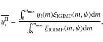 |
(14) |
where yi (m) is the yield of chemical element i produced by a single star of mass m (see also Goodwin & Pagel 2005 for a similar approach). The nucleosynthetic prescriptions are taken from Woosley & Weaver (1995). We have however halved the iron yields, in accordance with Timmes et al. (1995) and Chiappini et al. (1997), because it is known that only in this way it is possible to reproduce the [
![\begin{figure}
\par\includegraphics[width=8.5cm,clip]{1472fig9.eps}
\end{figure}](/articles/aa/full_html/2009/21/aa11472-08/img109.png) |
Figure 9:
IGIMF-averaged SNII yields of oxygen (solid
lines), iron (dotted lines) and magnesium (dashed lines) as a function
of SFR (in |
| Open with DEXTER | |
Once we know the SNIa yields and the IGIMF-averaged SNII yields for
each galaxy, we can calculate the mass fraction
![]() (where
(where ![]() is O or Mg) produced until the time t by using
the formula:
is O or Mg) produced until the time t by using
the formula:
where
At this point, we can compute the theoretical average stellar
abundances by means of:
![\begin{displaymath}[\alpha/{\rm Fe}]= \log_{10} \frac{\psi \cdot \int_{0}^{\Delt...
...}{M_{\rm tot}} - \log_{10}{\alpha_\odot
\over {\rm Fe}_\odot},
\end{displaymath}](/articles/aa/full_html/2009/21/aa11472-08/img114.png) |
(16) |
where
The observable in elliptical galaxies is the velocity dispersion instead of
the mass, so in order to properly compare our results with observations we
need to assume a correlation between the stellar mass and the velocity
dispersion of galaxies (Faber-Jackson relation). We assume:
 |
(17) |
(Burstein et al. 1997), where
In Fig. 10 we show our results for
![]() comparing our models with observations taken from THOM05 and references
therein (filled squares). We can first notice that, as expected, the model
BETA100 (heavy dashed lines), giving rise to flatter IGIMFs (see
Fig. 1), produces larger [
comparing our models with observations taken from THOM05 and references
therein (filled squares). We can first notice that, as expected, the model
BETA100 (heavy dashed lines), giving rise to flatter IGIMFs (see
Fig. 1), produces larger [![]() /Fe] ratios. In fact, flatter
IGIMFs result in a larger fraction of massive stars and, therefore, a larger
production of
/Fe] ratios. In fact, flatter
IGIMFs result in a larger fraction of massive stars and, therefore, a larger
production of ![]() -elements. We can also see that the models reproduce
quite well the [
-elements. We can also see that the models reproduce
quite well the [![]() /Fe] (both [O/Fe] and [Mg/Fe]) ratios in elliptical
galaxies, at least for the models BETA200 and BETA235. To appreciate the
effect of the IGIMF approach, we plot (long-dashed line) a model with the
fixed canonical IMF which, as mentioned in Sects. 2 and 3.2, has the form
/Fe] (both [O/Fe] and [Mg/Fe]) ratios in elliptical
galaxies, at least for the models BETA200 and BETA235. To appreciate the
effect of the IGIMF approach, we plot (long-dashed line) a model with the
fixed canonical IMF which, as mentioned in Sects. 2 and 3.2, has the form
![]() ,
with
,
with
![]() for
for
![]() and
and
![]() above
above
![]() .
The curves obtained with the IGIMF tend to flatten out at large
.
The curves obtained with the IGIMF tend to flatten out at large
![]() ,
whereas the curve obtained with a constant IMF shows a constant
slope. This demonstrates once more that the adoption of the IGIMF is
particularly remarkable in the low-mass (and low-
,
whereas the curve obtained with a constant IMF shows a constant
slope. This demonstrates once more that the adoption of the IGIMF is
particularly remarkable in the low-mass (and low-![]() )
galaxies. The
curve with a constant IMF asymptotically approaches the model BETA100 since
this model at large SFRs produces the flattest IMFs (see
Fig. 1). Besides a small shift of a few tenths of a dex (which
can be removed by increasing the parameter A in Eq. 10), the curve
with a constant IMF reproduces well the trend of [
)
galaxies. The
curve with a constant IMF asymptotically approaches the model BETA100 since
this model at large SFRs produces the flattest IMFs (see
Fig. 1). Besides a small shift of a few tenths of a dex (which
can be removed by increasing the parameter A in Eq. 10), the curve
with a constant IMF reproduces well the trend of [![]() /Fe] vs.
/Fe] vs. ![]() of
the THOM05 sample, demonstrating that the downsizing (or inverse-wind) models
(Matteucci 1994; Pipino & Matteucci 2004) are also able to
explain this trend in large elliptical galaxies. However, evidence is
mounting that [
of
the THOM05 sample, demonstrating that the downsizing (or inverse-wind) models
(Matteucci 1994; Pipino & Matteucci 2004) are also able to
explain this trend in large elliptical galaxies. However, evidence is
mounting that [![]() /Fe] ratios in early-type dwarf galaxies are solar or
sub-solar. For instance, van Zee et al. (2004) showed
that [
/Fe] ratios in early-type dwarf galaxies are solar or
sub-solar. For instance, van Zee et al. (2004) showed
that [![]() /Fe] ratios (derived from Lick indices) of a sample of Virgo
dwarf irregular galaxies range between -0.3 and solar. Also in the cluster
Abell 496 the smallest galaxies show [Mg/Fe] to be solar or sub-solar
(Chilingarian et al. 2008). To show this, we have also plotted in
Fig. 10 (open triangles) the data of a sample of low-mass
early-type galaxies by Sansom & Northeast (2008). These data confirm
that the [
/Fe] ratios (derived from Lick indices) of a sample of Virgo
dwarf irregular galaxies range between -0.3 and solar. Also in the cluster
Abell 496 the smallest galaxies show [Mg/Fe] to be solar or sub-solar
(Chilingarian et al. 2008). To show this, we have also plotted in
Fig. 10 (open triangles) the data of a sample of low-mass
early-type galaxies by Sansom & Northeast (2008). These data confirm
that the [![]() /Fe] vs.
/Fe] vs. ![]() relation is probably steeper in the
low-mass regime and that our IGIMF results can naturally predict this
behavior. However, in order to properly test our results in the low-mass
regime more data are needed.
relation is probably steeper in the
low-mass regime and that our IGIMF results can naturally predict this
behavior. However, in order to properly test our results in the low-mass
regime more data are needed.
In this figure (and in the following ones) we have considered only model
galaxies for which the SFR is lower than
![]() yr-1. This is the
reason why the data points reach larger
yr-1. This is the
reason why the data points reach larger ![]() than the results of our
model. In extreme starbursts the IMF might become top-heavy as shown by the
mass-to-light ratios in ultra-compact dwarf galaxies, which are ultra-massive
``star clusters'' that form when the SFR is very high (Dabringhausen et al. 2009); this will need to be incorporated in the IGIMF
calculations (work in preparation).
than the results of our
model. In extreme starbursts the IMF might become top-heavy as shown by the
mass-to-light ratios in ultra-compact dwarf galaxies, which are ultra-massive
``star clusters'' that form when the SFR is very high (Dabringhausen et al. 2009); this will need to be incorporated in the IGIMF
calculations (work in preparation).
![\begin{figure}
\par\includegraphics[width=12cm,clip]{1472fg10.eps}
\end{figure}](/articles/aa/full_html/2009/21/aa11472-08/img119.png) |
Figure 10:
Mass-weighted [Mg/Fe] ( upper panel) and
[O/Fe] ( lower panel) vs. |
| Open with DEXTER | |
In general, in local early-type galaxies the stellar abundances are measured
by means of various absorption-line Lick indices, such as Mg b and
![]() (THOM05). To properly compare predictions to
observational abundance data obtained for local ellipticals, in general one
should derive the luminosity-weighted average abundances. The real abundances
averaged by mass are larger than the luminosity-averaged ones, owing to the
fact that, at constant age, metal-poor stars are brighter (Greggio
1997). To calculate the luminosities we have made use of the
Starburst99 package (Leitherer et al. 1999; Vázquez & Leitherer
2005), producing L (t) for each value of SFR and
(THOM05). To properly compare predictions to
observational abundance data obtained for local ellipticals, in general one
should derive the luminosity-weighted average abundances. The real abundances
averaged by mass are larger than the luminosity-averaged ones, owing to the
fact that, at constant age, metal-poor stars are brighter (Greggio
1997). To calculate the luminosities we have made use of the
Starburst99 package (Leitherer et al. 1999; Vázquez & Leitherer
2005), producing L (t) for each value of SFR and ![]() .
The
results are shown in Fig. 11 for the first 100 Myr (the luminosities
remain almost constant after 100 Myr). As expected, since model BETA100 is
characterized by the flattest IGIMFs, it also produces the highest
luminosities. We then calculated luminosity-weighted mass ratios by using the
formula:
.
The
results are shown in Fig. 11 for the first 100 Myr (the luminosities
remain almost constant after 100 Myr). As expected, since model BETA100 is
characterized by the flattest IGIMFs, it also produces the highest
luminosities. We then calculated luminosity-weighted mass ratios by using the
formula:
![\begin{displaymath}[\alpha/{\rm Fe}]= \log_{10} \frac{\int_{0}^{\Delta t} {\alph...
... {\rm d}t} - \log_{10}{\alpha_\odot
\over {\rm Fe}_\odot}\cdot
\end{displaymath}](/articles/aa/full_html/2009/21/aa11472-08/img121.png)
The results are shown in Fig. 12. As we can see, the results differ very little (by a few hundredths of a dex at most) compared to the mass-averaged abundance ratios. We have checked these results using the spectro-photometric code of Jimenez et al. (1998; see also Calura & Matteucci 2003) but the results do not differ appreciably compared with the ones obtained with the Starburst99 package. Indeed, it has been already shown in the literature (but for constant IMFs) that the discrepancy in the [Mg/Fe] ratio computed by averaging by mass and by luminosity is very small, with typical values of 0.01 dex (Matteucci et al. 1998; Thomas et al. 1999). We have confirmed this finding in the case of the IGIMF.
![\begin{figure}
\par\includegraphics[width=8.5cm,clip]{1472fg11.eps}
\end{figure}](/articles/aa/full_html/2009/21/aa11472-08/img122.png) |
Figure 11:
Stellar luminosities (in |
| Open with DEXTER | |
![\begin{figure}
\par\includegraphics[width=8.5cm,clip]{1472fg12.eps}
\end{figure}](/articles/aa/full_html/2009/21/aa11472-08/img123.png) |
Figure 12:
As in Fig. 10 but with
luminosity-weighted [ |
| Open with DEXTER | |
To check how much our results depend on the assumption of a variable ![]() with stellar mass, we plot in Fig. 13 the [
with stellar mass, we plot in Fig. 13 the [![]() /Fe]
obtained assuming a constant value of
/Fe]
obtained assuming a constant value of
![]() Gyr. The agreement with
observations is still quite good; in particular the models maintain an
increasing trend of [
Gyr. The agreement with
observations is still quite good; in particular the models maintain an
increasing trend of [![]() /Fe] with
/Fe] with ![]() .
However, the curves tend to
flatten out too much at larger
.
However, the curves tend to
flatten out too much at larger ![]() ,
at variance with the trend shown by
the observations. This is due to the fact that, as pointed out in
Sect. 2, the various IGIMFs for rates of star formation larger
than
,
at variance with the trend shown by
the observations. This is due to the fact that, as pointed out in
Sect. 2, the various IGIMFs for rates of star formation larger
than ![]() yr-1 do not show very large differences. Therefore, the
assumption of a star formation duration inversely proportional to the stellar
mass of the galaxy (or in other words the downsizing) is a key ingredient to
understand the chemical properties of large elliptical galaxies.
yr-1 do not show very large differences. Therefore, the
assumption of a star formation duration inversely proportional to the stellar
mass of the galaxy (or in other words the downsizing) is a key ingredient to
understand the chemical properties of large elliptical galaxies.
![\begin{figure}
\par\includegraphics[width=8.5cm,clip]{1472fg13.eps}
\end{figure}](/articles/aa/full_html/2009/21/aa11472-08/img124.png) |
Figure 13:
As in Fig. 10 but with
|
| Open with DEXTER | |
To appreciate the dependence on the distribution function of mass ratios in
binary stars (the parameter ![]() introduced in Sect. 3.2) we
plot in Figs. 14 and 15 the results
of models with
introduced in Sect. 3.2) we
plot in Figs. 14 and 15 the results
of models with
![]() and
and
![]() ,
respectively. The curves
obtained with
,
respectively. The curves
obtained with
![]() tend to be slightly steeper than the ones shown
in Fig. 10 (and slightly steeper than the observations)
but the agreement still remains good, in particular for the models BETA100 and
BETA200. If we assume
tend to be slightly steeper than the ones shown
in Fig. 10 (and slightly steeper than the observations)
but the agreement still remains good, in particular for the models BETA100 and
BETA200. If we assume
![]() ,
an excellent match to the observations
is instead provided by the model BETA235. Models BETA100 and BETA200 show the
same slope of the observational data but shifted by a few tenths of a dex. A
slight increase of the parameter A in Eq. (10) would make these
models perfectly compatible with the observations.
,
an excellent match to the observations
is instead provided by the model BETA235. Models BETA100 and BETA200 show the
same slope of the observational data but shifted by a few tenths of a dex. A
slight increase of the parameter A in Eq. (10) would make these
models perfectly compatible with the observations.
It is particularly remarkable that the trend of [![]() /Fe] ratios
vs.
/Fe] ratios
vs. ![]() (namely an increase of [
(namely an increase of [![]() /Fe] with
/Fe] with ![]() )
is naturally
reproduced using the IGIMF approach, without any further assumption or
fine-tuning of parameters. This is for instance at variance with what
hierarchical clustering models of structure formation would tend to produce,
since in this case larger elliptical galaxies are formed later, out of
building blocks in which the [
)
is naturally
reproduced using the IGIMF approach, without any further assumption or
fine-tuning of parameters. This is for instance at variance with what
hierarchical clustering models of structure formation would tend to produce,
since in this case larger elliptical galaxies are formed later, out of
building blocks in which the [![]() /Fe] ratio has already dropped (e.g.
Thomas et al. 2002). De Lucia et al. (2006), by means of a
semi-analytical model adopting the concordance
/Fe] ratio has already dropped (e.g.
Thomas et al. 2002). De Lucia et al. (2006), by means of a
semi-analytical model adopting the concordance ![]() CDM cosmology,
suggested that more massive ellipticals should have shorter star formation
timescales, but lower assembly (by dry mergers) redshift than less luminous
systems. This is one of the first works based on the hierarchical paradigm
for galaxy formation producing downsizing in the star formation histories of
early-type galaxies through the inclusion of AGN feedback (see also Bower et al. 2006; Cattaneo et al. 2006), although they did not
compute the [
CDM cosmology,
suggested that more massive ellipticals should have shorter star formation
timescales, but lower assembly (by dry mergers) redshift than less luminous
systems. This is one of the first works based on the hierarchical paradigm
for galaxy formation producing downsizing in the star formation histories of
early-type galaxies through the inclusion of AGN feedback (see also Bower et al. 2006; Cattaneo et al. 2006), although they did not
compute the [![]() /Fe]-
/Fe]-![]() relation for ellipticals. However, the
lower assembly redshift for the most massive system is still in contrast to
what is concluded by Cimatti et al. (2006), who show that
the downsizing trend should be extended also to the mass assembly, in the
sense that the most massive ellipticals should have assembled before the less
massive ones. Very recently, Pipino et al. (2008) showed that even in
semi-analytical models able to account for the downsizing, the [
relation for ellipticals. However, the
lower assembly redshift for the most massive system is still in contrast to
what is concluded by Cimatti et al. (2006), who show that
the downsizing trend should be extended also to the mass assembly, in the
sense that the most massive ellipticals should have assembled before the less
massive ones. Very recently, Pipino et al. (2008) showed that even in
semi-analytical models able to account for the downsizing, the [![]() /Fe]
vs.
/Fe]
vs. ![]() relation is not reproduced.
relation is not reproduced.
![\begin{figure}
\par\includegraphics[width=8.5cm,clip]{1472fg14.eps}
\end{figure}](/articles/aa/full_html/2009/21/aa11472-08/img126.png) |
Figure 14:
As in Fig. 10 but with
|
| Open with DEXTER | |
![\begin{figure}
\par\includegraphics[width=8.5cm,clip]{1472fg15.eps}
\end{figure}](/articles/aa/full_html/2009/21/aa11472-08/img127.png) |
Figure 15:
As in Fig. 10 but
with
|
| Open with DEXTER | |
Although the agreement between our results and the observations is good, none
of the models presented so far fits perfectly the data at low and high
![]() simultaneously. In order to work out an overall best model, for each
value of
simultaneously. In order to work out an overall best model, for each
value of ![]() and
and ![]() we checked, by means of a minimization of the
normalized chi square, which normalization constant A better fits the data.
The results are shown in Fig. 16. As we can see, model BETA235 seems
to be preferable and the best agreement between data and models is obtained
for the model BETA235 with
we checked, by means of a minimization of the
normalized chi square, which normalization constant A better fits the data.
The results are shown in Fig. 16. As we can see, model BETA235 seems
to be preferable and the best agreement between data and models is obtained
for the model BETA235 with
![]() and A = 0.036. In general, the
best fits are obtained with large values of
and A = 0.036. In general, the
best fits are obtained with large values of ![]() ,
although that requires
low values of A. A large value of
,
although that requires
low values of A. A large value of ![]() ,
favoring equal-mass binary
systems, is consistent with the results of Shara & Hurley (2002),
although observational surveys cited in Sect. 3.2 seem to indicate
lower values of
,
favoring equal-mass binary
systems, is consistent with the results of Shara & Hurley (2002),
although observational surveys cited in Sect. 3.2 seem to indicate
lower values of ![]() .
.
![\begin{figure}
\par\includegraphics[width=8.5cm,clip]{1472fg16.eps}
\end{figure}](/articles/aa/full_html/2009/21/aa11472-08/img128.png) |
Figure 16:
Normalization constant A to adopt in order to
obtain the best fit with the observational data as a function of |
| Open with DEXTER | |
However we should not forget that the ![]() -luminous mass relation we
have used in this work has been obtained by THOM05 assuming a constant
IMF. We have therefore checked, starting from our best model, namely a
model with
-luminous mass relation we
have used in this work has been obtained by THOM05 assuming a constant
IMF. We have therefore checked, starting from our best model, namely a
model with
![]() ,
,
![]() and A = 0.036, how this relation
should change in order to best fit the data. It turns out that, within the
IGIMF theory, the best
and A = 0.036, how this relation
should change in order to best fit the data. It turns out that, within the
IGIMF theory, the best ![]() -luminous mass relation is given by:
-luminous mass relation is given by:
where
![\begin{figure}
\par\includegraphics[width=8.5cm,clip]{1472fg17.eps}
\end{figure}](/articles/aa/full_html/2009/21/aa11472-08/img131.png) |
Figure 17:
Mass-weighted [Mg/Fe] ( upper panel) and [O/Fe]
( lower panel) vs. |
| Open with DEXTER | |
![\begin{figure}
\par\includegraphics[width=8.5cm,clip]{1472fg18.eps}
\end{figure}](/articles/aa/full_html/2009/21/aa11472-08/img132.png) |
Figure 18:
|
| Open with DEXTER | |
5 Discussion and conclusions
In this paper we have studied, by means of analytical and semi-analytical
calculations, the evolution of [![]() /Fe] ratios in early-type galaxies and
in particular their dependence on the luminous mass (or equivalently on the
velocity dispersion
/Fe] ratios in early-type galaxies and
in particular their dependence on the luminous mass (or equivalently on the
velocity dispersion ![]() ). We have applied the so-called integrated
galactic initial mass function (IGIMF, Kroupa & Weidner 2003; Weidner
& Kroupa 2005) theory, namely we have assumed that the IMF depends on
the star formation rate (SFR) of the galaxy, in the sense that the larger the
SFR, the flatter the resulting slope of the IGIMF. This kind of behavior
would naturally tend to form more massive stars (and therefore more SNeII) in
large galaxies, which are characterized by more intense star formation
episodes. Therefore, it is expected that, since
). We have applied the so-called integrated
galactic initial mass function (IGIMF, Kroupa & Weidner 2003; Weidner
& Kroupa 2005) theory, namely we have assumed that the IMF depends on
the star formation rate (SFR) of the galaxy, in the sense that the larger the
SFR, the flatter the resulting slope of the IGIMF. This kind of behavior
would naturally tend to form more massive stars (and therefore more SNeII) in
large galaxies, which are characterized by more intense star formation
episodes. Therefore, it is expected that, since ![]() -elements are mostly
formed by SNeII, the most massive galaxies are also the ones which attain the
largest [
-elements are mostly
formed by SNeII, the most massive galaxies are also the ones which attain the
largest [![]() /Fe] ratios, in agreement with the observations. One of the
main aims of this paper was to quantitatively check whether the chemical
evolution of galaxies within the IGIMF theory is able to accurately fit the
observed [
/Fe] ratios, in agreement with the observations. One of the
main aims of this paper was to quantitatively check whether the chemical
evolution of galaxies within the IGIMF theory is able to accurately fit the
observed [![]() /Fe] vs.
/Fe] vs. ![]() relation.
relation.
We have analytically calculated the SNII and SNIa rates with the IGIMF
assuming 3 possible slopes of the distribution function of embedded clusters,
![]() ,
where
,
where
![]() is the
stellar mass of the embedded star cluster; in particular we have considered
is the
stellar mass of the embedded star cluster; in particular we have considered
![]() (model BETA100);
(model BETA100);
![]() (model BETA200);
(model BETA200);
![]() (model BETA235). We have seen that, if we consider constant SFRs over the
whole Hubble time, the final SNIa and SNII rates agree quite well with the
observations of spiral galaxies (in particular the S0a/b ones). The agreement
with the observed rates in irregular galaxies is not good, but a constant SFR
over the whole Hubble time is not likely in irregular galaxies, which probably
have experienced an increase of the SFR in the last Gyrs of their evolution.
(model BETA235). We have seen that, if we consider constant SFRs over the
whole Hubble time, the final SNIa and SNII rates agree quite well with the
observations of spiral galaxies (in particular the S0a/b ones). The agreement
with the observed rates in irregular galaxies is not good, but a constant SFR
over the whole Hubble time is not likely in irregular galaxies, which probably
have experienced an increase of the SFR in the last Gyrs of their evolution.
To calculate the [![]() /Fe] ratios with the IGIMF we assumed that
early-type galaxies form stars at a constant rate over a period of time
/Fe] ratios with the IGIMF we assumed that
early-type galaxies form stars at a constant rate over a period of time
![]() which depends on the total luminous mass of the considered galaxy.
This hypothesis is based on the work of THOM05 who, on the basis of
observational grounds, showed the existence of a downsizing pattern for
elliptical galaxies, i.e. that the most massive galaxies are the ones with the
shortest
which depends on the total luminous mass of the considered galaxy.
This hypothesis is based on the work of THOM05 who, on the basis of
observational grounds, showed the existence of a downsizing pattern for
elliptical galaxies, i.e. that the most massive galaxies are the ones with the
shortest ![]() .
We then calculated the production of
.
We then calculated the production of ![]() -elements
and Fe by SNeII (in particular we calculated IGIMF-averaged SNII yields) and
by SNeIa and we calculated mass-weighted and luminosity-weighted [
-elements
and Fe by SNeII (in particular we calculated IGIMF-averaged SNII yields) and
by SNeIa and we calculated mass-weighted and luminosity-weighted [![]() /Fe]
ratios for each model galaxy, characterized by different SFRs and
/Fe]
ratios for each model galaxy, characterized by different SFRs and ![]() .
.
The resulting mass-averaged [![]() /Fe] vs.
/Fe] vs. ![]() relations show the same
slope as the observations in massive galaxies as reported by THOM05,
irrespective of the value of
relations show the same
slope as the observations in massive galaxies as reported by THOM05,
irrespective of the value of ![]() and of the distribution function of mass
ratios in binaries
and of the distribution function of mass
ratios in binaries
![]() (which affects the SNIa
rates), although models with
(which affects the SNIa
rates), although models with
![]() and large values of
and large values of ![]() seem
to be preferable. Some models show a shift (of a few tenths of a dex)
compared with the observations but this can be fixed increasing (or
decreasing) the fraction, A, of binary systems giving rise to SNeIa, which
is an almost unconstrained parameter. It is however remarkable that all the
models we have calculated show the same trend of the observations because if,
as commonly argued, large elliptical galaxies form out of mergers of smaller
sub-structures (hierarchical clustering), it would be natural to expect that
they are the ones with the lowest [
seem
to be preferable. Some models show a shift (of a few tenths of a dex)
compared with the observations but this can be fixed increasing (or
decreasing) the fraction, A, of binary systems giving rise to SNeIa, which
is an almost unconstrained parameter. It is however remarkable that all the
models we have calculated show the same trend of the observations because if,
as commonly argued, large elliptical galaxies form out of mergers of smaller
sub-structures (hierarchical clustering), it would be natural to expect that
they are the ones with the lowest [![]() /Fe] ratios because they form
later, out of building blocks where [
/Fe] ratios because they form
later, out of building blocks where [![]() /Fe] has already dropped.
/Fe] has already dropped.
It is worth pointing out that the [![]() /Fe] ratios do not depend on the
gas flows (infall and outflow) experienced by the galaxy (Recchi et al. 2008) therefore our results do not depend on specific infall and
outflow parameters, which make them particularly robust. However, these
parameters affect the overall metallicity of the galaxy, therefore they need
to be taken into account in order to check whether our models can correctly
reproduce the mass-metallicity relation. As mentioned in the Introduction,
Köppen et al. (2007) have already shown that the IGIMF theory is
able to reproduce the mass-metallicity relation found by Tremonti et al. (2004) in star-forming galaxies. We are checking, by means of
detailed numerical models, that the IGIMF theory is able to reproduce at the
same time the mass-metallicity relation and the [
/Fe] ratios do not depend on the
gas flows (infall and outflow) experienced by the galaxy (Recchi et al. 2008) therefore our results do not depend on specific infall and
outflow parameters, which make them particularly robust. However, these
parameters affect the overall metallicity of the galaxy, therefore they need
to be taken into account in order to check whether our models can correctly
reproduce the mass-metallicity relation. As mentioned in the Introduction,
Köppen et al. (2007) have already shown that the IGIMF theory is
able to reproduce the mass-metallicity relation found by Tremonti et al. (2004) in star-forming galaxies. We are checking, by means of
detailed numerical models, that the IGIMF theory is able to reproduce at the
same time the mass-metallicity relation and the [![]() /Fe]-
/Fe]-![]() relation in early-type galaxies. This study will be presented in a
forthcoming paper.
relation in early-type galaxies. This study will be presented in a
forthcoming paper.
We have also considered models in which the IMF does not vary with the SFR
and, because of the variations of ![]() with SFR, these models are
compatible with the observations of large elliptical galaxies as well.
However, these models produce a [
with SFR, these models are
compatible with the observations of large elliptical galaxies as well.
However, these models produce a [![]() /Fe] vs.
/Fe] vs. ![]() relation that can
be described as a single-slope power-law, whereas the IGIMF models bend
significantly at low masses (and low
relation that can
be described as a single-slope power-law, whereas the IGIMF models bend
significantly at low masses (and low ![]() ). This is because the IGIMF
becomes particularly steep in the galaxies with the mildest SFRs and this adds
to the downsizing effect (namely the decreasing duration of the SFR with
increasing mass). From our study therefore, an important conclusion is that a
very reliable observable to test the validity of the IGIMF theory is the
observation of the [
). This is because the IGIMF
becomes particularly steep in the galaxies with the mildest SFRs and this adds
to the downsizing effect (namely the decreasing duration of the SFR with
increasing mass). From our study therefore, an important conclusion is that a
very reliable observable to test the validity of the IGIMF theory is the
observation of the [![]() /Fe] ratios in dwarf galaxies. The available data
on [
/Fe] ratios in dwarf galaxies. The available data
on [![]() /Fe] ratios in low-mass early-type galaxies indeed show some
steepening of the [
/Fe] ratios in low-mass early-type galaxies indeed show some
steepening of the [![]() /Fe] vs.
/Fe] vs. ![]() relation, in agreement with the
IGIMF predictions.
relation, in agreement with the
IGIMF predictions.
We have also tested how much our results depend on the assumption of a
variable ![]() with stellar mass by computing models with
with stellar mass by computing models with
![]() Gyr irrespective of the stellar mass. The agreement between models and
observational data is still reasonably good but the curves tend to flatten out
too much at large stellar masses compared with the observations (and with the
IGIMF models). This indicates that the downsizing remains a fundamental
ingredient to understand the chemical properties of early-type galaxies.
However, if we check for which
Gyr irrespective of the stellar mass. The agreement between models and
observational data is still reasonably good but the curves tend to flatten out
too much at large stellar masses compared with the observations (and with the
IGIMF models). This indicates that the downsizing remains a fundamental
ingredient to understand the chemical properties of early-type galaxies.
However, if we check for which ![]() -luminous mass relation we obtain
the best fit between data and models, it turns out that the downsizing effect
must be milder than predicted by THOM05, in the sense that large galaxies form
stars for a slightly longer timescale than calculated by THOM05, whereas
low-mass galaxies have star formation durations significantly shorter.
Although the exact form of the best-fit
-luminous mass relation we obtain
the best fit between data and models, it turns out that the downsizing effect
must be milder than predicted by THOM05, in the sense that large galaxies form
stars for a slightly longer timescale than calculated by THOM05, whereas
low-mass galaxies have star formation durations significantly shorter.
Although the exact form of the best-fit ![]() -luminous mass relation is
subject to a number of parameters (IGIMF parameters; parameters regulating the
SNIa rate etc.) and might change once larger and more detailed abundance
measurements are available, the result of a milder downsizing effect compared
to the findings of THOM05 is robust.
-luminous mass relation is
subject to a number of parameters (IGIMF parameters; parameters regulating the
SNIa rate etc.) and might change once larger and more detailed abundance
measurements are available, the result of a milder downsizing effect compared
to the findings of THOM05 is robust.
Thus, we have seen that luminosity-weighted [![]() /Fe] ratios agree very
well with the mass-weighted ones (with relative differences of a few
hundredths of dex at most), in accordance with the results of Matteucci et al. (1998).
/Fe] ratios agree very
well with the mass-weighted ones (with relative differences of a few
hundredths of dex at most), in accordance with the results of Matteucci et al. (1998).
We remind the reader that, with our analytical approach to chemical evolution,
we are making some important simplifying assumptions. For instance, our
computation of the interstellar
![]() given by
Eq. (15) does not take into account in detail the lifetimes of
massive stars. Furthermore, our present calculations do not take into account
the variation with time of the metallicity in galaxies, which should also
influence the stellar yields. From the various tests performed so far, and
from the comparison of our results with numerical results (Thomas et al. 1999; Pipino & Matteucci 2004), we have verified that
these assumptions may play only some minor role in determining the zero-point,
but not the slope of the predicted [
given by
Eq. (15) does not take into account in detail the lifetimes of
massive stars. Furthermore, our present calculations do not take into account
the variation with time of the metallicity in galaxies, which should also
influence the stellar yields. From the various tests performed so far, and
from the comparison of our results with numerical results (Thomas et al. 1999; Pipino & Matteucci 2004), we have verified that
these assumptions may play only some minor role in determining the zero-point,
but not the slope of the predicted [![]() /Fe] vs.
/Fe] vs. ![]() relation. All of
these simplifying assumptions will be relaxed in our forthcoming paper, where
we will present a numerical approach to the role of the IGIMF in galactic
chemical evolution.
relation. All of
these simplifying assumptions will be relaxed in our forthcoming paper, where
we will present a numerical approach to the role of the IGIMF in galactic
chemical evolution.
The main results of our paper can be summarized as follows:
- Models in which the IGIMF theory is implemented naturally reproduce an
increasing trend of [/Fe] with luminous mass (or
 ), as
observed in early-type galaxies.
), as
observed in early-type galaxies.
- However, models with constant duration of the star formation produce a
[/Fe] vs.
relation which flattens out too much at large
.
Only models in which the star formation duration inversely
correlates with the galactic luminous mass (downsizing) can quantitatively
reproduce the observations.
- Models in which the IGIMF is implemented show (at variance with the
constant IMF models) a steepening of the [/Fe] vs.
relation
for small galaxies, therefore the IGIMF theory can be tested by observing
the [/Fe] in dwarf galaxies. The observations available so far are
in agreement with our predictions.
- Luminosity-weighted abundance ratios differ from the mass-weighted ones
by a few hundredths of dex at most. This result, already known for constant
IMF models, has been confirmed in the IGIMF framework.
- In order to obtain the best fit between our results and the observed
[/Fe] ratios in early-type galaxies, the downsizing effect (namely
the shorter duration of the star formation in larger galaxies) has to be
milder than previously thought.
- The best results are obtained for a cluster mass function
 ,
indicating that the embedded cluster mass
function should have a Salpeter slope.
,
indicating that the embedded cluster mass
function should have a Salpeter slope.
Acknowledgements
We warmly thank Francesca Matteucci for help and support. Discussions with Antonio Pipino are also acknowledged. S.R. acknowledges generous financial support from the FWF through the Lise Meitner grant M1079-N16. F.C. and S.R. acknowledge financial support from PRIN2007 (Italian Ministry of Research) Prot. N. 2007JJC53X. We thank the referee, Daniel Thomas, for very useful comments.
References
- Abt, H. A., & Levy, S. G. 1976, ApJS, 30, 273 [NASA ADS] [CrossRef]
- Anders, E., & Grevesse, N. 1989, Geochim. Cosmochim. Acta, 53, 197 [NASA ADS] [CrossRef] (In the text)
- Bower, R. G., Benson, A. J., Malbon, R., et al. 2006, MNRAS, 370, 645 [NASA ADS] (In the text)
- Burstein, D., Bender, R., Faber, S., & Nolthenius, R. 1997, AJ, 114, 1365 [NASA ADS] [CrossRef] (In the text)
- Calura, F., & Matteucci, F. 2003, ApJ, 596, 734 [NASA ADS] [CrossRef] (In the text)
- Calura, F., & Matteucci, F. 2006, ApJ, 652, 889 [NASA ADS] [CrossRef] (In the text)
- Calura, F., Matteucci, F., & Menci, N. 2004, MNRAS, 353, 500 [NASA ADS] [CrossRef] (In the text)
- Cattaneo, A., Dekel, A., Devriendt, J., Guiderdoni, B., & Blaizot, J. 2006, MNRAS, 370, 1651 [NASA ADS] (In the text)
- Chabrier, G. 2001, ApJ, 554, 1274 [NASA ADS] [CrossRef] (In the text)
- Chiappini, C., Matteucci, F., & Gratton, R. 1997, ApJ, 477, 765 [NASA ADS] [CrossRef] (In the text)
- Chilingarian, I. V., Cayatte, V., Durret, F., et al. 2008, A&A, 486, 85 [NASA ADS] [CrossRef] [EDP Sciences] (In the text)
- Cimatti, A., Daddi, E., & Renzini, A. 2006, A&A, 453, 29 [NASA ADS] [CrossRef] (In the text)
- Cowie, L. L., Songalia, A., Hu, E. M., & Cohen, J. G. 1996, AJ, 112, 839 [NASA ADS] [CrossRef] (In the text)
- Dabringhausen, J., Kroupa, P., & Baumgardt, H. 2009, MNRAS, 394, 1529 [NASA ADS] [CrossRef] (In the text)
- De Lucia, G., Springel, V., White, S. D. M., Croton, D., & Kauffmann, G. 2006, MNRAS, 366, 499 [NASA ADS] [CrossRef] (In the text)
- Duquennoy, A., & Mayor, M. 1991, A&A, 248, 485 [NASA ADS] (In the text)
- Evans, N. J., & Dunham, M. M. 2009, ApJS, 181, 321 [NASA ADS] [CrossRef] (In the text)
- Gibson, B. K., Loewenstein, M., & Mushotzky, R. F. 1997, MNRAS, 290, 623 [NASA ADS] (In the text)
- Goodwin, S. P., & Pagel, B. E. J. 2005, MNRAS, 359, 707 [NASA ADS] [CrossRef] (In the text)
- Greggio, L. 1997, MNRAS, 285, 151 [NASA ADS] (In the text)
- Greggio, L. 2005, A&A, 441, 1055 [NASA ADS] [CrossRef] [EDP Sciences] (In the text)
- Greggio, L., & Renzini, A. 1983, A&A, 118, 217 [NASA ADS] (In the text)
- Hunter, D. A., Elmegreen, B. G., Dupuy, T. J., & Mortonson, M. 2003, AJ, 126, 1836 [NASA ADS] [CrossRef] (In the text)
- Jimenez, R., Padoan, P., Matteucci, F., & Heavens, A. F. 1998, MNRAS, 299, 123 [NASA ADS] [CrossRef] (In the text)
- Kodama, T., Yamada, T., Akiyama, M., et al. 2004, MNRAS, 350, 1005 [NASA ADS] [CrossRef] (In the text)
- Köppen, J., Weidner, C., & Kroupa, P. 2007, MNRAS, 375, 673 [NASA ADS] [CrossRef] (In the text)
- Kouwenhoven, M. B. N., Brown, A. G. A., Zinnecker, H., Kaper, L., & Portegies Zwart, S. F. 2005, A&A, 430, 137 [NASA ADS] [CrossRef] [EDP Sciences] (In the text)
- Kroupa, P., & Weidner, C. 2003, ApJ, 598, 1076 [NASA ADS] [CrossRef] (In the text)
- Kroupa, P., Tout, C. A., & Gilmore, G. 1993, MNRAS, 262, 545 [NASA ADS] (In the text)
- Kuntschner, H., Lucey, J. R., Smith, R. J., Hudson, R. J., & Davies, R. L. 2001, MNRAS, 323, 615 [NASA ADS] [CrossRef] (In the text)
- Lada, C. J., & Lada, E. A. 2003, ARA&A, 41, 57 [NASA ADS] [CrossRef] (In the text)
- Larsen, S. S., & Richtler, T. 2000, A&A, 354, 836 [NASA ADS] (In the text)
- Larsen, T. I., Sommer-Larsen, J., & Pagel, B. E. J. 2001, MNRAS, 323, 555 [NASA ADS] [CrossRef] (In the text)
- Leitherer, C., Schaerer, D., Goldader, J. D., et al. 1999, ApJS, 123, 3 [NASA ADS] [CrossRef] (In the text)
- Mannucci, F., Della Valle, M., Panagia, N., et al. 2005, A&A, 433, 807 [NASA ADS] [CrossRef] [EDP Sciences] (In the text)
- Maoz, D. 2008, MNRAS, 384, 267 [NASA ADS] [CrossRef] (In the text)
- Marigo, P. 2001, A&A, 370, 194 [NASA ADS] [CrossRef] [EDP Sciences] (In the text)
- Massey, P. 2003, ARA&A, 41, 15 [NASA ADS] [CrossRef] (In the text)
- Massey, P., & Hunter, D. A. 1998, ApJ, 493, 180 [NASA ADS] [CrossRef] (In the text)
- Matteucci, F. 1994, A&A, 288, 57 [NASA ADS] (In the text)
- Matteucci, F. 2001, The Chemical Evolution of the Galaxy, ASSL (Kluwer Academic Publisher) (In the text)
- Matteucci, F. 2007, [arXiv:0704.0770] (In the text)
- Matteucci, F., & Recchi, S. 2001, ApJ, 558, 351 [NASA ADS] [CrossRef] (In the text)
- Matteucci, F., Ponzone, R., & Gibson, B. K. 1998, A&A, 335, 855 [NASA ADS] (In the text)
- Nagashima, M., Lacey, C. G., Okamoto, T., et al. 2005, MNRAS, 363, L31 [NASA ADS] (In the text)
- Padovani, P., & Matteucci F. 1993, ApJ, 416, 26 [NASA ADS] [CrossRef] (In the text)
- Pflamm-Altenburg, J., Weidner, C., & Kroupa, P. 2007, ApJ, 671, 1550 [NASA ADS] [CrossRef] (PWK07) (In the text)
- Pilyugin, L. S., & Edmunds, M. G. 1996, A&A, 313, 783 [NASA ADS] (In the text)
- Pipino, A., & Matteucci, F. 2004, MNRAS, 347, 968 [NASA ADS] [CrossRef] (In the text)
- Pipino, A., Kawata, D., Gibson, B. K., & Matteucci, F. 2005, A&A, 434, 553 [NASA ADS] [CrossRef] [EDP Sciences] (In the text)
- Pipino, A., Devriendt, J. E. G., Thomas, D., Silk, J., & Kaviraj, S. 2008, [arXiv:0810.5753] (In the text)
- Pipino, A., Silk, J., & Matteucci, F. 2009, MNRAS, 392, 475 [NASA ADS] [CrossRef] (In the text)
- Piskunov, A. E., Belikov, A. N., Kharchenko, N. V., Sagar, R., & Subramaniam, A. 2004, MNRAS, 349, 1449 [NASA ADS] [CrossRef] (In the text)
- Recchi, S., Spitoni, E., Matteucci, F., & Lanfranchi, G. A. 2008, A&A, 489, 555 [NASA ADS] [CrossRef] [EDP Sciences] (In the text)
- Romano, D., Chiappini, C., Matteucci, F., & Tosi, M. 2005, A&A, 430, 491 [NASA ADS] [CrossRef] [EDP Sciences] (In the text)
- Salpeter, E. E. 1955, ApJ, 121, 161 [NASA ADS] [CrossRef] (In the text)
- Sansom, A. E., & Northeast, M. S. 2008, MNRAS, 387, 331 [NASA ADS] [CrossRef] (In the text)
- Shara, M. M., & Hurley, J. R. 2002, ApJ, 571, 830 [NASA ADS] [CrossRef] (In the text)
- Shatsky, N., & Tokovinin, A. 2002, A&A, 382, 92 [NASA ADS] [CrossRef] [EDP Sciences] (In the text)
- Siess, L. 2007, A&A, 476, 893 [NASA ADS] [CrossRef] [EDP Sciences] (In the text)
- Smith, L. J., & Gallagher, J. S. III 2001, MNRAS, 326, 1027 [NASA ADS] [CrossRef] (In the text)
- Thielemann, F. -K., Nomoto, K., & Hashimoto, M. 1993, in Origin and Evolution of the Elements, ed. N. Prantzos, E. Vangioni-Flam, & M. Cassé (Cambridge: Cambridge Univ. Press), 297 (In the text)
- Thomas, D., Greggio, L., & Bender, R. 1999, MNRAS, 302, 537 [NASA ADS] [CrossRef] (In the text)
- Thomas, D., Maraston, C., & Bender, R. 2002, Ap&SS, 281, 371 [NASA ADS] [CrossRef] (In the text)
- Thomas, D., Maraston, C., Bender, R., & Mendes de Oliveira, C. 2005, ApJ, 621, 673 [NASA ADS] [CrossRef] (THOM05) (In the text)
- Timmes, F. X., Woosley, S. E., & Weaver, T. A. 1995, ApJS, 98, 617 [NASA ADS] [CrossRef] (In the text)
- Tremonti, C. A., Heckman, T. M., Kauffmann, G., et al. 2004, ApJ, 613, 898 [NASA ADS] [CrossRef] (In the text)
- Tutukov, A.V. 1978, A&A, 70, 57 [NASA ADS] (In the text)
- Tutukov, A. V., & Yungelson, L. R. 1980, in Close Binary Stars, ed. M. J. PLavec, D. M. Popper, & R. K. Ulrich (Dordrecht: Reidel), 15 (In the text)
- Valiante, R., Matteucci, F., Recchi, S., & Calura, F. 2009, New Astron., 14, 638 [NASA ADS] [CrossRef] (In the text)
- van Zee, L., Barton, E. J., & Skillman, E. D. 2004, AJ, 128, 2797 [NASA ADS] [CrossRef] (In the text)
- Vázquez, G. A., & Leitherer, C. 2005, ApJ, 621, 695 [NASA ADS] [CrossRef] (In the text)
- Weidner, C., & Kroupa, P. 2004, MNRAS, 348, 187 [NASA ADS] [CrossRef] (In the text)
- Weidner, C., & Kroupa, P. 2005, ApJ, 625, 754 [NASA ADS] [CrossRef] (In the text)
- Weidner, C., & Kroupa, P. 2006, MNRAS, 365, 1333 [NASA ADS] (In the text)
- Weidner, C., Kroupa, P., & Larsen, S.S. 2004, MNRAS, 350, 1503 [NASA ADS] [CrossRef] (In the text)
- Weiss, A., Peletier, R. F., & Matteucci, F. 1995, A&A, 296, 73 [NASA ADS] (In the text)
- Whelan, J., & Iben, I. Jr. 1973, ApJ, 186, 1007 [NASA ADS] [CrossRef] (In the text)
- Woosley, S. E., & Weaver, T. A. 1995, ApJS, 101, 181 [NASA ADS] [CrossRef] (In the text)
- Wyse, R. F. G., Gilmore, G., Houdashelt, M. L., et al. 2002, New Astron., 7, 395 [NASA ADS] [CrossRef] (In the text)
- Zhang, Q., & Fall, S. M. 1999, ApJ, 527, L81 [NASA ADS] [CrossRef] (In the text)
Footnotes
- ... parameter
![[*]](/icons/foot_motif.png)
- Note that observational papers usually
adopt mass ratios
q = m2/m1 instead of
 (Abt & Levy 1976).
The mass ratio distribution function f (q) can be obtained from
(Abt & Levy 1976).
The mass ratio distribution function f (q) can be obtained from  by means of a simple change of variable.
All Figures
| |
Figure 1:
IGIMFs for different distributions of embedded
clusters (e.g. different values of |
| Open with DEXTER | |
| In the text | |
| |
Figure 2:
IGIMFs for different SFRs: |
| Open with DEXTER | |
| In the text | |
| |
Figure 3:
Lower panel:
|
| Open with DEXTER | |
| In the text | |
| |
Figure 4:
Lower panel:
|
| Open with DEXTER | |
| In the text | |
| |
Figure 5:
|
| Open with DEXTER | |
| In the text | |
| |
Figure 6:
|
| Open with DEXTER | |
| In the text | |
| |
Figure 7:
As in Fig. 6 but for
|
| Open with DEXTER | |
| In the text | |
| |
Figure 8:
Duration |
| Open with DEXTER | |
| In the text | |
| |
Figure 9:
IGIMF-averaged SNII yields of oxygen (solid
lines), iron (dotted lines) and magnesium (dashed lines) as a function
of SFR (in |
| Open with DEXTER | |
| In the text | |
| |
Figure 10:
Mass-weighted [Mg/Fe] ( upper panel) and
[O/Fe] ( lower panel) vs. |
| Open with DEXTER | |
| In the text | |
| |
Figure 11:
Stellar luminosities (in |
| Open with DEXTER | |
| In the text | |
| |
Figure 12:
As in Fig. 10 but with
luminosity-weighted [ |
| Open with DEXTER | |
| In the text | |
| |
Figure 13:
As in Fig. 10 but with
|
| Open with DEXTER | |
| In the text | |
| |
Figure 14:
As in Fig. 10 but with
|
| Open with DEXTER | |
| In the text | |
| |
Figure 15:
As in Fig. 10 but
with
|
| Open with DEXTER | |
| In the text | |
| |
Figure 16:
Normalization constant A to adopt in order to
obtain the best fit with the observational data as a function of |
| Open with DEXTER | |
| In the text | |
| |
Figure 17:
Mass-weighted [Mg/Fe] ( upper panel) and [O/Fe]
( lower panel) vs. |
| Open with DEXTER | |
| In the text | |
| |
Figure 18:
|
| Open with DEXTER | |
| In the text | |
Copyright ESO 2009
Current usage metrics show cumulative count of Article Views (full-text article views including HTML views, PDF and ePub downloads, according to the available data) and Abstracts Views on Vision4Press platform.
Data correspond to usage on the plateform after 2015. The current usage metrics is available 48-96 hours after online publication and is updated daily on week days.
Initial download of the metrics may take a while.