| Issue |
A&A
Volume 499, Number 3, June I 2009
|
|
|---|---|---|
| Page(s) | 697 - 710 | |
| Section | Extragalactic astronomy | |
| DOI | https://doi.org/10.1051/0004-6361/200811118 | |
| Published online | 25 March 2009 | |
Recovery of the star formation history of the LMC from the VISTA survey of the Magellanic system
L. O. Kerber1,2 - L. Girardi1 - S. Rubele1,3 - M.-R. Cioni4 (for the VMC Team)
1 - Osservatorio Astronomico di Padova - INAF, Vicolo dell'Osservatorio 5, 35122 Padova, Italy
2 - Universidade de São Paulo, IAG, Rua do Matão 1226, Cidade Universitária, São Paulo 05508-900, Brazil
3 -
Dipartimento di Astronomia, Università di Padova, Vicolo dell'Osservatorio 2, 35122 Padova, Italy
4 - Center for Astrophysics Research, University of Hertfordshire, Hatfield AL10 9AB, UK
Received 9 October 2008 / Accepted 12 January 2009
Abstract
The VISTA near infrared survey of the Magellanic System (VMC) will
provide deep
![]() photometry reaching stars in the oldest
turn-off point throughout the Magellanic Clouds (MCs).
As part of the preparation for the survey, we aim to access the
accuracy in the star formation history (SFH) that can be expected from
VMC data, in particular for the Large Magellanic Cloud (LMC).
To this aim, we first simulate VMC images containing not only the LMC
stellar populations but also the foreground Milky Way (MW) stars and
background galaxies. The simulations cover the whole range of density
of LMC field stars. We then perform aperture photometry over these
simulated images, access the expected levels of photometric errors and
incompleteness, and apply the classical technique of
SFH-recovery based on the reconstruction of colour-magnitude diagrams
(CMD) via the minimisation of a chi-squared-like statistics. We verify
that the foreground MW stars are accurately recovered by the
minimisation algorithms, whereas the background galaxies can be
largely eliminated from the CMD analysis due to their particular
colours and morphologies.
We then evaluate the expected errors in the recovered star formation
rate as a function of stellar age, SFR(t), starting from models with
a known age-metallicity relation (AMR). It turns out that, for a
given sky area, the random errors for ages older than
photometry reaching stars in the oldest
turn-off point throughout the Magellanic Clouds (MCs).
As part of the preparation for the survey, we aim to access the
accuracy in the star formation history (SFH) that can be expected from
VMC data, in particular for the Large Magellanic Cloud (LMC).
To this aim, we first simulate VMC images containing not only the LMC
stellar populations but also the foreground Milky Way (MW) stars and
background galaxies. The simulations cover the whole range of density
of LMC field stars. We then perform aperture photometry over these
simulated images, access the expected levels of photometric errors and
incompleteness, and apply the classical technique of
SFH-recovery based on the reconstruction of colour-magnitude diagrams
(CMD) via the minimisation of a chi-squared-like statistics. We verify
that the foreground MW stars are accurately recovered by the
minimisation algorithms, whereas the background galaxies can be
largely eliminated from the CMD analysis due to their particular
colours and morphologies.
We then evaluate the expected errors in the recovered star formation
rate as a function of stellar age, SFR(t), starting from models with
a known age-metallicity relation (AMR). It turns out that, for a
given sky area, the random errors for ages older than ![]() 0.4 Gyr
seem to be independent of the crowding. This can be explained by a
counterbalancing effect between the loss of stars from a decrease in
the completeness and the gain of stars from an increase in the
stellar density. For a spatial resolution of
0.4 Gyr
seem to be independent of the crowding. This can be explained by a
counterbalancing effect between the loss of stars from a decrease in
the completeness and the gain of stars from an increase in the
stellar density. For a spatial resolution of ![]()
![]() ,
the
random errors in SFR(t) will be below 20% for this wide range of
ages. On the other hand, due to the lower stellar statistics for
stars younger than
,
the
random errors in SFR(t) will be below 20% for this wide range of
ages. On the other hand, due to the lower stellar statistics for
stars younger than ![]() 0.4 Gyr, the outer LMC regions will require
larger areas to achieve the same level of accuracy in the SFR(t). If
we consider the AMR as unknown, the SFH-recovery algorithm is able to
accurately recover the input AMR, at the price of an increase of
random errors in the SFR(t) by a factor of about 2.5. Experiments of
SFH-recovery performed for varying distance modulus and reddening
indicate that these parameters can be determined with (relative)
accuracies of
0.4 Gyr, the outer LMC regions will require
larger areas to achieve the same level of accuracy in the SFR(t). If
we consider the AMR as unknown, the SFH-recovery algorithm is able to
accurately recover the input AMR, at the price of an increase of
random errors in the SFR(t) by a factor of about 2.5. Experiments of
SFH-recovery performed for varying distance modulus and reddening
indicate that these parameters can be determined with (relative)
accuracies of
![]() mag and
mag and
![]() mag,
for each individual field over the LMC. The propagation of these
errors in the SFR(t) implies systematic errors below 30%.
This level of accuracy in the SFR(t) can reveal significant
imprints in the dynamical evolution of this unique and nearby stellar system,
as well as possible signatures of the past interaction between the MCs
and the MW.
mag,
for each individual field over the LMC. The propagation of these
errors in the SFR(t) implies systematic errors below 30%.
This level of accuracy in the SFR(t) can reveal significant
imprints in the dynamical evolution of this unique and nearby stellar system,
as well as possible signatures of the past interaction between the MCs
and the MW.
Key words: galaxies: evolution - Magellanic Clouds - surveys - infrared: stars: Hertzsprung-Russell (HR) and C-M diagrams - methods: numerical
1 Introduction
Determining the star formation histories (SFH) of the Magellanic Clouds (MC) is one of the most obvious goals in the study of nearby galaxies, for several reasons. First, this SFH probably keeps a record of the past interactions between both the Clouds and the Milky Way (Holtzman et al. 1999; Harris & Zaritsky 2004; Smecker-Hane et al. 2002; Olsen 1999), which are still to be properly unveiled (Piatek et al. 2008; Kallivayalil et al. 2006a,b; Besla et al. 2007). Detailed SFH studies may also provide invaluable hints to how star formation is triggered and proceeds in time, from the smallest to galactic-size scales, and to how these processes depend on dynamical effects (e.g. Harris 2007a; Harris & Zaritsky 2008).
The Magellanic Clouds are also a rich laboratory for studying of star formation and evolution and the calibration of primary standard candles, thanks to the simultaneous presence of a wide variety of interesting objects such as red clump giants, Cepheids, RR Lyrae, long-period variables, carbon stars, planetary nebulae, the tip of the red giant branch (RGB), dust-enshrouded giants, and pre-main sequence stars. Although the system contains several hundred star clusters for which age and metallicity can be measured, the bulk of the interesting stellar objects are actually in the field, irremediably mixed by the complex SFH, and partially hidden by the presence of variable and patchy extinction across the MCs. Unveiling this complex SFH may help in calibrating stellar properties - luminosities, lifetimes, periods, chemical types, etc. - as a function of age and metallicity.
In the past two decades, many authors have demonstrated that recovering the SFH of the MC from optical photometry is indeed feasible and well worth the effort. Such works are, usually, based either on deep Hubble Space Telescope (HST) photometry reaching the oldest main sequence turn-off for small MC areas (e.g. Ardeberg et al. 1997; Elson et al. 1997; Smecker-Hane et al. 2002; Gallagher et al. 1996; Olsen 1999; Holtzman et al. 1999; Javiel et al. 2005; Dolphin et al. 2001) or on relatively shallow ground-based photometry covering larger areasover the MCs (Stappers et al. 1997; Harris & Zaritsky 2004,2001; Gardiner & Hatzidimitriou 1992). Only in a very few cases (e.g. Gallart et al. 2004; Noël et al. 2007) have the ground-based optical photometry been deep enough to reach the oldest main sequence turn-offs.
The VISTA Survey of the Magellanic System![]() (VMC, see Cioni et al. 2008, Cioni et al., in
preparation) is an ESO public survey project which will
provide, in the next 5 years, critical near-infrared data aimed -
among other goals - to improve upon present-day SFH determinations.
This will hopefully pave the way to a more complete understanding of
how star formation relates to the dynamical processes under way in the
system and to more accurate calibration of stellar models and
primary standard candles. Regarding the SFH, the key contributions of
the VMC Survey will: (1) provide photometry reaching as
deep as the oldest main sequence turn-off over the bulk of the
MC system, as opposed to the tiny regions sampled by HST, and the
limited area covered by most of the dedicated ground-based
observations; (2) use the near-infrared
(VMC, see Cioni et al. 2008, Cioni et al., in
preparation) is an ESO public survey project which will
provide, in the next 5 years, critical near-infrared data aimed -
among other goals - to improve upon present-day SFH determinations.
This will hopefully pave the way to a more complete understanding of
how star formation relates to the dynamical processes under way in the
system and to more accurate calibration of stellar models and
primary standard candles. Regarding the SFH, the key contributions of
the VMC Survey will: (1) provide photometry reaching as
deep as the oldest main sequence turn-off over the bulk of the
MC system, as opposed to the tiny regions sampled by HST, and the
limited area covered by most of the dedicated ground-based
observations; (2) use the near-infrared
![]() passbands, hopefully reducing the errors in the SFH-recovery due to
variable extinction across the MCs.
passbands, hopefully reducing the errors in the SFH-recovery due to
variable extinction across the MCs.
On the other hand, the use of near-infrared instead of optical filters
will introduce some complicating factors, like a higher degree of
contamination of the MC photometry by foreground stars and background
galaxies, and the extremely high noise contributed by the sky,
especially in the ![]() band.
band.
Indeed, VMC will be the first near-infrared wide-area survey to
provide data suitable for the classical methods of
SFH-recovery![]() . With the new space-based near-infrared cameras
(the HST/WFC3 IR channel, and JWST) and ground-based adaptive optics
facilities, observations similar to VMC ones will likely be available
for many nearby galaxies. VMC may become the precursor of detailed
SFH-recovery in the opening window of near-infrared
wavelengths. Demonstrating the feasibility of VMC goals, therefore, is
of more general interest.
. With the new space-based near-infrared cameras
(the HST/WFC3 IR channel, and JWST) and ground-based adaptive optics
facilities, observations similar to VMC ones will likely be available
for many nearby galaxies. VMC may become the precursor of detailed
SFH-recovery in the opening window of near-infrared
wavelengths. Demonstrating the feasibility of VMC goals, therefore, is
of more general interest.
Another particularity of the VMC Survey is that, once started, its data flow will be so huge that algorithms of analysis need to be prepared in advance, in the form of semi-automated pipelines. Similar approaches have been followed by some ambitious nearly-all-sky (SDSS, 2MASS), micro-lensing (MACHO, OGLE, EROS), and space astrometry (e.g. Hipparcos, GAIA) surveys.
In this paper, we describe part of the preparatory work for deriving of the SFH from VMC data, which can be summarised in the following way. First we simulate the VMC images for the LMC (Sect. 2), where we later perform the photometry and artificial stars tests (Sect. 3) that allow us to access the expected levels of photometric errors, completeness, and crowding, and the contamination by foreground stars and background galaxies. We then proceed with many experiments of SFH-recovery (Sect. 4), evaluating the uncertainties in the derivation of the SFH as a function of basic quantities such as the stellar density over the LMC, the area included in the analysis, and the adopted values for the distance and reddening. Doing this, we are able to present the expected random and systematic errors in the space-resolved SFH. This information may be useful to plan complementary observations and surveys of the LMC in the next few years. Subsequent papers will present the perspectives for the Small Magellanic Cloud (SMC), as well as explore the effect better on the recovered SFH by the uncertainties associated with the MC geometry, differential reddening, initial mass function, fraction of binaries, etc.
2 Simulating VMC data
Our initial goal is to obtain realistic simulations of VMC images, containing all of the objects that are known to be present towards the MCs and likely to be detectable within the survey's depth limits. These objects are essentially stars belonging to the MW and the MCs and background galaxies. Moreover, an essential component of the images is the high signal from the infrared sky. Each one of these components will be described below. Diffuse objects such as emission nebulae and star clusters will be ignored for the moment.
2.1 VISTA and VMC specifications
VMC will be performed with the VIRCAM camera mounted at the 4m VISTA
telescope at ESO's Paranal Observatory in Chile.
VIRCAM has
![]() detectors that cover a sky area
of 0.037
detectors that cover a sky area
of 0.037
![]() each with the image scale of 0.339
each with the image scale of 0.339
![]() per
pixel on average.
The basic mode of the observations will
be to perform 6 exposures (paw-prints) with the subsequent construction
of
per
pixel on average.
The basic mode of the observations will
be to perform 6 exposures (paw-prints) with the subsequent construction
of
![]()
![]() tiles. In the following, we adopt the
area of each detector (i.e. 0.037
tiles. In the following, we adopt the
area of each detector (i.e. 0.037
![]() )
as the basic unit of our
simulations.
)
as the basic unit of our
simulations.
The specifications of the VMC Survey will be described in detail
in another paper (Cioni et al., in preparation).
For our aims, suffice it to mention that,
despite the crowded fields, the observations are expected to be
sky-noise dominated. The mean sky brightness
at Cerro Paranal is of 17.2, 16.0, 13.0 mag arcsec-2 in
![]() ,
respectively. The required seeing is 1.0
,
respectively. The required seeing is 1.0
![]() (FWHM) in the
Y band, being the most crowded regions observed in nights with seeing better than 0.8
(FWHM) in the
Y band, being the most crowded regions observed in nights with seeing better than 0.8
![]() .
The targetted signal-to-noise ratio (SNR) is equal to 10 at magnitudes
of 21.9, 21.4, 20.3 mag. The photometric zero-points in
our simulations were fixed via the VISTA exposure time calculator, so
as to be consistent with these values. Considering these survey limits, in our simulations we include all objects brighter than
.
The targetted signal-to-noise ratio (SNR) is equal to 10 at magnitudes
of 21.9, 21.4, 20.3 mag. The photometric zero-points in
our simulations were fixed via the VISTA exposure time calculator, so
as to be consistent with these values. Considering these survey limits, in our simulations we include all objects brighter than
![]() ,
which at the LMC distance correspond to a stellar mass of
,
which at the LMC distance correspond to a stellar mass of ![]() 0.8
0.8 ![]() in the main
sequence turn-off.
in the main
sequence turn-off.
![\begin{figure}
\par\includegraphics[width=8cm,clip]{1111801.eps}
\end{figure}](/articles/aa/full_html/2009/21/aa11118-08/img42.png) |
Figure 1:
The area VMC will likely cover in the LMC (solid line) and SMC (dashed line) as a function of the surface density of RGB stars,
|
| Open with DEXTER | |
VMC tiles will cover most of the Magellanic System,
summing to a total area of 184
![]() (see Cioni et al. 2008, and Cioni et al., in
preparation, for details). Figure 1 shows
a histogram of the total area to be observed as a function of the
density of upper RGB stars,
(see Cioni et al. 2008, and Cioni et al., in
preparation, for details). Figure 1 shows
a histogram of the total area to be observed as a function of the
density of upper RGB stars,
![]() ,
which is defined as the
number of 2MASS stars inside a box in the
,
which is defined as the
number of 2MASS stars inside a box in the ![]() vs.
vs.
![]() CMD (
CMD (
![]() and
and
![]() for the LMC and
for the LMC and
![]() for the SMC), for each unit area of 0.05
for the SMC), for each unit area of 0.05
![]() .
Notice the
higher mean and maximum stellar densities of the LMC, as compared to
the SMC. The stellar densities vary over an interval of about 2.5 dex.
.
Notice the
higher mean and maximum stellar densities of the LMC, as compared to
the SMC. The stellar densities vary over an interval of about 2.5 dex.
2.2 Stars in the UKIDSS photometric system
Since VISTA is still being commissioned at the time of writing, the
throughputs of VISTA filters, camera, and telescope are still not
available. It is, however, clear that the VISTA photometric system will
be very similar to the UKIDSS one, with the differences mainly
in the higher performance of VISTA and in the fact that VISTA will
use a K-short filter (![]() )
similar to the 2MASS one.
)
similar to the 2MASS one.
Given the present situation, we have so far used the UKIDSS system as
a surrogate of the future VISTA one. Tests using the preliminary VISTA
filter curves (Jim Emerson, private communication) indicate very small
differences in the synthetic photometry, typically smaller than
0.02 mag, between VISTA and UKIDSS![]() .
.
![\begin{figure}
\par\includegraphics[width=8.5cm,clip]{1111802.eps}
\end{figure}](/articles/aa/full_html/2009/21/aa11118-08/img49.png) |
Figure 2:
A series of Marigo et al. (2008) isochrones in the UKIDSS photometric system. The figure shows the absolute (MK,
|
| Open with DEXTER | |
Stellar isochrones in the UKIDSS system have been recently provided by
Marigo et al. (2008)![]() . The
conversion to the UKIDSS system takes not only the
photospheric emission from stars into account, but also the
reprocessing of their radiation by dusty shells in mass-losing stars,
as described in Marigo et al. (2008).
The filter transmission curves and zero-point
definitions come from Hewett et al. (2006). The stellar models in use
are composed of the Girardi et al. (2000) tracks for low- and
intermediate-mass stars, replacing the thermally pulsing asymptotic
giant branch (AGB) evolution with the Marigo & Girardi (2007) ones. In this
paper, these models are further complemented with white and brown
dwarfs as described in Girardi et al. (2005, <)586#>also Zabot et al., in
preparation#, and with the Bertelli et al. (1994)
isochrones for masses higher than 7
. The
conversion to the UKIDSS system takes not only the
photospheric emission from stars into account, but also the
reprocessing of their radiation by dusty shells in mass-losing stars,
as described in Marigo et al. (2008).
The filter transmission curves and zero-point
definitions come from Hewett et al. (2006). The stellar models in use
are composed of the Girardi et al. (2000) tracks for low- and
intermediate-mass stars, replacing the thermally pulsing asymptotic
giant branch (AGB) evolution with the Marigo & Girardi (2007) ones. In this
paper, these models are further complemented with white and brown
dwarfs as described in Girardi et al. (2005, <)586#>also Zabot et al., in
preparation#, and with the Bertelli et al. (1994)
isochrones for masses higher than 7 ![]() .
Figure 2
presents some of the Marigo et al. (2008) isochrones in the MKvs.
.
Figure 2
presents some of the Marigo et al. (2008) isochrones in the MKvs.
![]() diagram, for a wide range in age and metallicity.
As readily noticed, the isochrones contain the vast majority of the
single objects that can be prominent in the near-infrared observations
of the LMC, going from the lower main-sequence (MS) stars
up to the brightest AGB stars and red supergiants.
The stellar masses in the MS and the apparent magnitude for a
typical LMC distance,
diagram, for a wide range in age and metallicity.
As readily noticed, the isochrones contain the vast majority of the
single objects that can be prominent in the near-infrared observations
of the LMC, going from the lower main-sequence (MS) stars
up to the brightest AGB stars and red supergiants.
The stellar masses in the MS and the apparent magnitude for a
typical LMC distance,
![]() (Schaefer 2008; Alves 2004; Clementini et al. 2003), are also indicated in
this figure. We recall that our models contain, in addition, the
very low-mass stars, brown dwarfs, and white dwarfs, which are
important in the description of the foreground MW population
(Marigo et al. 2003).
(Schaefer 2008; Alves 2004; Clementini et al. 2003), are also indicated in
this figure. We recall that our models contain, in addition, the
very low-mass stars, brown dwarfs, and white dwarfs, which are
important in the description of the foreground MW population
(Marigo et al. 2003).
The interstellar extinction coefficients adopted in this work also
follow from Marigo et al. (2008):
AY=0.385 AV,
AJ=0.283 AV,
and
AK=0.114 AV, which imply
![]() and
and
![]() .
They have been derived from synthetic photometry
applied to a G2V star extincted with the Cardelli et al. (1989)
extinction curve. Although the approach is not the most accurate one
(see Girardi et al. 2008), it is appropriate to the conditions of
the moderate reddening (
.
They have been derived from synthetic photometry
applied to a G2V star extincted with the Cardelli et al. (1989)
extinction curve. Although the approach is not the most accurate one
(see Girardi et al. 2008), it is appropriate to the conditions of
the moderate reddening (
![]() mag) typical of the Magellanic
Clouds.
mag) typical of the Magellanic
Clouds.
The simulation of the input photometric catalogues and the generation
of artificial images are described in the next sections. In brief,
the input catalogues for the LMC (Sect. 2.3) and the
foreground MW stars (Sect. 2.4) come from the
predictions made with the TRILEGAL code (Girardi et al. 2005),
which simulates the photometry of resolved stellar populations following
a given distribution of initial masses, ages, metallicities, reddenings,
and distances. The catalogues of background galaxies
(Sect. 2.5) are randomly drawn from UKIDSS
(Lawrence et al. 2007). The simulation of images is performed with
the DAOPHOT and ARTDATA packages in IRAF![]() (Sect. 2.6), always respecting the photometric
calibration and expected image quality required by the VMC Survey.
(Sect. 2.6), always respecting the photometric
calibration and expected image quality required by the VMC Survey.
2.3 The LMC stars
The stellar populations for the LMC are simulated as an ``additional object'' inside the TRILEGAL code (Girardi et al. 2005), where the input parameters for a field are:
- the star formation rate as a function of stellar age, SFR(t);
- the stellar AMR, Z(t) or [M/H](t);
- the total stellar mass,
 ;
;
- the distance modulus,
 ;
;
- the reddening,
 ;
;
- the initial mass function (IMF),
 ;
;
- the fraction of detached unresolved binaries,
 .
.
In the LMC simulations presented in this paper, we adopt an input AMR consistent with the one given by stellar clusters (Kerber et al. 2007; Grocholski et al. 2006; Mackey & Gilmore 2003; Olszewski et al. 1991) and field stars (Carrera et al. 2008; Cole et al. 2005), together with a constant SFR(t). Since the SFR(t) in the LMC is clearly spatially dependent (Javiel et al. 2005; Holtzman et al. 1999; Smecker-Hane et al. 2002), the assumption of a constant SFR(t) is just considered as a way to ensure a uniform treatment for all stellar populations over the LMC.
In terms of distance we are initially using the canonical value of
![]() (Schaefer 2008; Alves 2004; Clementini et al. 2003), also
adopted by the HST Key Project to measure the Hubble constant
(Freedman et al. 2001), whereas for the reddening we are assuming a
value of
(Schaefer 2008; Alves 2004; Clementini et al. 2003), also
adopted by the HST Key Project to measure the Hubble constant
(Freedman et al. 2001), whereas for the reddening we are assuming a
value of
![]() ,
typical of the extinction maps from
Schlegel et al. (1998). For real VMC
images, these two parameters are expected to be free parameters, since
the LMC presents disk-like geometries with a significant inclination
(
,
typical of the extinction maps from
Schlegel et al. (1998). For real VMC
images, these two parameters are expected to be free parameters, since
the LMC presents disk-like geometries with a significant inclination
(![]() 30-40 deg) (van der Marel & Cioni 2001; Nikolaev et al. 2004; van der Marel et al. 2002)
and non-uniform extinction (Zaritsky et al. 2004; Imara & Blitz 2007; Subramaniam 2005).
30-40 deg) (van der Marel & Cioni 2001; Nikolaev et al. 2004; van der Marel et al. 2002)
and non-uniform extinction (Zaritsky et al. 2004; Imara & Blitz 2007; Subramaniam 2005).
Finally the assumed values for the remaining inputs are the
Chabrier (2001) lognormal
IMF![]() and
and
![]() % with a constant mass
ratio distribution for
m2/m1 > 0.7
% with a constant mass
ratio distribution for
m2/m1 > 0.7![]() . There are no strong reasons to expect
significant deviations for these choices, especially for the IMF, since
we are dealing with stars with masses approximately between 0.8 and
12.0
. There are no strong reasons to expect
significant deviations for these choices, especially for the IMF, since
we are dealing with stars with masses approximately between 0.8 and
12.0
![]() where the IMF slope seems to be universal
and similar to the Salpeter one (Kroupa 2002,2001).
Concerning the fraction of binaries, our choice is
consistent with the values found for the stellar clusters in the LMC
(Elson et al. 1998). For the moment, these will be
considered as fixed inputs. Later papers will use simulations
to quantify the systematic errors in the recovered SFH
introduced by the uncertainties related to these choices.
where the IMF slope seems to be universal
and similar to the Salpeter one (Kroupa 2002,2001).
Concerning the fraction of binaries, our choice is
consistent with the values found for the stellar clusters in the LMC
(Elson et al. 1998). For the moment, these will be
considered as fixed inputs. Later papers will use simulations
to quantify the systematic errors in the recovered SFH
introduced by the uncertainties related to these choices.
2.4 The Milky Way foreground
The MW foreground stars are simulated using the TRILEGAL code as described in Girardi et al. (2005). Towards the MCs, the simulated stars are located both in a disk with scale-height increasing with age and in a oblate halo component. Diffuse interstellar reddening within 100 pc of the Galactic plane is also considered, although it hardly affects the near-infrared photometry.
In Girardi et al. (2005), it has been shown that, for off-plane
lines-of-sight, TRILEGAL predicts star counts accurate to within about
15% over a wide range of magnitudes and down to
![]() and
and
![]() .
This accuracy is confirmed by the
.
This accuracy is confirmed by the ![]() observations of Gullieuszik et al. (2008) for a field next to the
Leo II dwarf spheroidal galaxy. Moreover, Marigo et al. (2003) shows
that TRILEGAL describes the position of the three ``vertical
fingers'' observed in 2MASS K vs.
observations of Gullieuszik et al. (2008) for a field next to the
Leo II dwarf spheroidal galaxy. Moreover, Marigo et al. (2003) shows
that TRILEGAL describes the position of the three ``vertical
fingers'' observed in 2MASS K vs.
![]() diagrams very well.
Similarly comforting comparisons with UKIDSS data (including the Yband) are presented in Sect. 3.2 below.
diagrams very well.
Similarly comforting comparisons with UKIDSS data (including the Yband) are presented in Sect. 3.2 below.
Although predicting star counts with an accuracy of about 15% may be good enough for our initial purposes, we are working to improve this accuracy further. In short, we are applying the minimisation algorithm described in Vanhollebeke et al. (2009) - successfully applied to the derivation of bulge parameters using data for inner MW regions - to recalibrate the TRILEGAL disk and halo models. It is likely that, before VMC starts, foreground star counts will be predicted with accuracies of about 5%.
2.5 The background galaxies
To simulate the population of galaxies background to the MCs,
we make use of the large catalogues of real galaxies obtained by the
UKIDSS Ultra-Deep (UDS; Foucaud et al. 2007) and Large Area Surveys
(LAS; Warren et al. 2007), from their Data Release 3 (December 2007). The
LAS includes data for an area of 4000
![]() down to K=18.4, for
YJK filters, whereas the UDS includes an area of 0.77
down to K=18.4, for
YJK filters, whereas the UDS includes an area of 0.77
![]() observed down to
observed down to ![]() ,
but only for JHK passbands.
,
but only for JHK passbands.
In our input catalogue for each simulation, we include the number of
UKIDSS galaxies expected for our total simulated area. More precisely,
we randomly pick from the UDS catalogue a fraction of galaxies
given by the ratio between the areas covered by UDS and by our image
simulation. From the catalogue, we extract their J and Kmagnitudes and morphological parameters (position angle, size, and
axial ratio). In this way, our simulations respect the observed
K-band luminosity function of galaxies and their J-K colour
distribution, down to faint magnitudes. The Y-band magnitudes,
instead, have been assigned in the following way. We take the J-Kcolour of each galaxy in the UDS and then randomly select a galaxy
from the LAS that has the most similar J-K (within 0.2 mag), and
take its Y-J. This means that the Y-J vs. J-K relation from LAS
is being extrapolated down to deeper magnitudes![]() .
.
2.6 Simulating images
Once we defined the input catalogues for stars and galaxies, we simulated the images inside IRAF, in accordance with the VISTA and VMC specifications (see Sect. 2.1). The basic sequence of steps (and the IRAF task) performed for a given filter is the following:
- 1.
- definition of the image size (rtextimage) and introduction of the sky brightness and noise (mknoise);
- 2.
- simulation of a Gaussian stellar profile (gauss) respecting the expected seeing for an image of a photometric-calibrated (using the VISTA ETC v1.3) delta function with a known number of electrons;
- 3.
- addition of the LMC and MW stars in the sky images (addstars) following the previously calibrated Gaussian stellar profile with random Poissonian errors in the number of electrons;
- 4.
- addition of galaxies (mkobject) in the previous image respecting all information concerning the morphological type, position angle, size, and axial ratio.
![\begin{figure}
\par\includegraphics[width=8cm,clip]{1111803a.eps}\par\mbox{\incl...
...idth=4cm]{1111803b.eps}\includegraphics[width=4cm]{1111803c.eps} }\end{figure}](/articles/aa/full_html/2009/21/aa11118-08/img73.png) |
Figure 3:
An image simulation for the area next to the star cluster NGC 1805 (
|
| Open with DEXTER | |
3 Performing photometry on simulated data
3.1 Aperture and PSF photometry
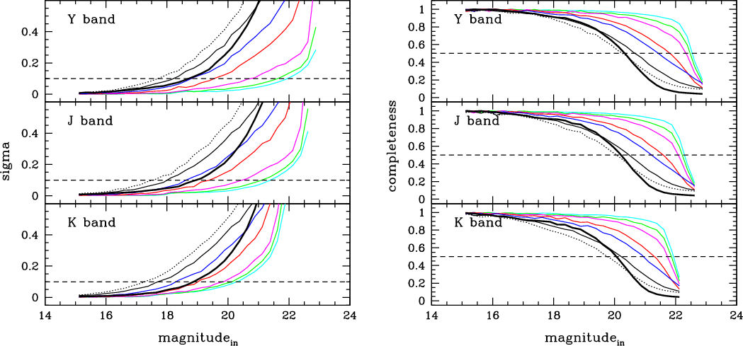 |
Figure 4:
Photometric errors ( left panels) and completeness curves ( right panels) in the artificial YJK images for the LMC for different levels of crowding. The thin curves present the results for
the aperture photometry covering the entire expected range of density
of field stars (
|
| Open with DEXTER | |
The IRAF DAOPHOT package was used to detect and to perform aperture
photometry in our simulated images. Candidate stars were detected
using daofind, with a peak intensity threshold for detection set
to
![]() ,
where
,
where
![]() corresponds to the
rms fluctuation in the sky counts. The aperture photometry was carried
out running the task phot for an aperture radius of 3 pix (
corresponds to the
rms fluctuation in the sky counts. The aperture photometry was carried
out running the task phot for an aperture radius of 3 pix (![]()
![]() ).
).
The photometric errors and completeness curves that come from this
aperture photometry in our simulated LMC images can be seen in
Fig. 4.
The photometric errors in this case were estimated using the differences
between the input and output magnitudes; more specifically, for each
small magnitude bin, we computed the half-width of the error
distribution with respect to the median,
which comprises 70% of the recovered stars. The completeness
is simply defined instead as the ratio between total number of input stars,
and those recovered by the photometry package.
Figure 4 presents the results for different simulations covering a wide range of density for field stars in the LMC, from the outer disk regions to the centre regions in the bar (see Fig. 1). In these simulations, we are following the requirement that the most central and crowded regions (
![]() )
will only be observed under excellent seeing conditions.
)
will only be observed under excellent seeing conditions.
It can be noticed that the VMC expected magnitudes at SNR=10 for
isolated stars (Y=21.9, J=21.4, K=20.3) is recovered in the
simulations for the regions with the lowest density, attesting the correct
photometric calibration of our simulated images. For these regions the
50% completeness level is reached at
![]() ,
,
![]() ,
and
,
and
![]() .
.
Crowding significantly affects the quality of the aperture
photometry, making the stars measured in central LMC regions appear
significantly brighter and have larger photometric errors than in
the outermost LMC regions.
As shown in Fig. 4, crowding clearly starts to
dominate the noise for fields with
![]() ,
which correspond to about 20% (7%) of the total area covered in the LMC (SMC)
(see Fig. 1).
Therefore, PSF photometry is expected to be
performed whenever crowding will prevent a good aperture photometry
over VMC images. The significant improvements that can be reach by a
PSF photometry are also illustrated by the thick black lines in
Fig. 4. These results
correspond to a PSF photometry applied to the LMC centre (
,
which correspond to about 20% (7%) of the total area covered in the LMC (SMC)
(see Fig. 1).
Therefore, PSF photometry is expected to be
performed whenever crowding will prevent a good aperture photometry
over VMC images. The significant improvements that can be reach by a
PSF photometry are also illustrated by the thick black lines in
Fig. 4. These results
correspond to a PSF photometry applied to the LMC centre (
![]() ), where the PSF fitting and the photometry were done using
the IRAF tasks psf and allstar.
), where the PSF fitting and the photometry were done using
the IRAF tasks psf and allstar.
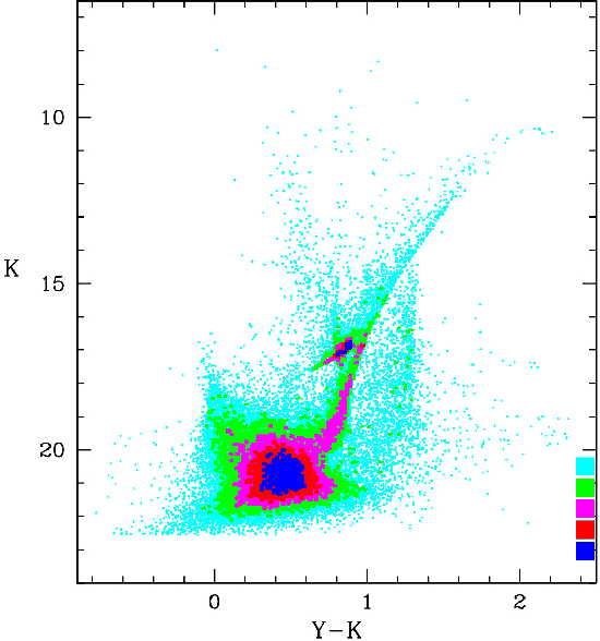 |
Figure 5:
Example of (K,
|
| Open with DEXTER | |
Figure 5 shows an example of CMD obtained from the
aperture photometry in a simulated field with an intermediate level of
density in the LMC. This figure reveals the expected CMD features - and the wealth of information - that will become available thanks to
the VMC Survey: well evident are the AGB, red supergiants, RGB, red
clump (RC), sub-giant branch (SGB) as well as the MS, from the
brightest and youngest stars down to the oldest turn-off point. In
comparison, the present-day near-infrared surveys of the MCs are
only complete for the most evolved stars - excluding those in the
most crowded regions and those highly extincted by circumstellar
dust. DENIS and 2MASS, for instance, are limited to
![]() ,
revealing the red supergiants, AGB, and upper RGB, and including just a
tiny fraction of the upper MS (Cioni et al. 2008; Nikolaev & Weinberg 2000). IRSF
(Kato et al. 2007) extends this range down to
,
revealing the red supergiants, AGB, and upper RGB, and including just a
tiny fraction of the upper MS (Cioni et al. 2008; Nikolaev & Weinberg 2000). IRSF
(Kato et al. 2007) extends this range down to
![]() ,
which is deep enough to sample the RC and RGB bump, but not the SGB
and the low-mass MS.
,
which is deep enough to sample the RC and RGB bump, but not the SGB
and the low-mass MS.
3.2 Comparison with UKIDSS data
Since the present work depends on simulations, it is important to check whether they reproduce the basic characteristics of real data already obtained under similar conditions. UKIDSS represents the most similar data to VMC available for the moment. Therefore, in the following we compare a simulated UKIDSS field with the real one.
For this exercise, we take the 0.21
![]() field towards Galactic
coordinates
field towards Galactic
coordinates
![]() ,
which due to its similar distance from
the Galactic plane as the MCs, offers a good opportunity to test the
expected levels of Milky Way foreground and the galaxy background.
,
which due to its similar distance from
the Galactic plane as the MCs, offers a good opportunity to test the
expected levels of Milky Way foreground and the galaxy background.
 |
Figure 6:
A comparison between the aperture photometry
from UKIDSS image data ( left) and the corresponding simulation
( right) for a 0.21
|
| Open with DEXTER | |
We took the original image from the UKIDSS archive and
performed aperture photometry with both DAOPHOT (Stetson 1987) ad
SExtractor (Bertin & Arnouts 1996). An image for the same area was
simulated using UKIDSS specifications (pixel scale, SNR, etc.) and
submitted to the same kind of catalogue
extraction. Figure 6 shows the results, after comparing the K vs.
![]() diagrams for the UKIDSS observed (left panel) and simulated
(right panel) fields for both stars (blue points) and galaxies (red
points). Stars and galaxies were separated using the SExtractor
Stellarity parameter st. We adopted st>0.85 for stars and
diagrams for the UKIDSS observed (left panel) and simulated
(right panel) fields for both stars (blue points) and galaxies (red
points). Stars and galaxies were separated using the SExtractor
Stellarity parameter st. We adopted st>0.85 for stars and
![]() for galaxies.
for galaxies.
Both DAOPHOT ad SExtractor aperture photometries turned out to be
remarkably consistent with the ones provided by the Cambridge
Astronomical Survey Unit (CASU) data reduction pipeline. This is very
comforting since the CASU will adopt the same data reduction pipeline
to the future VISTA data. The histograms at the right and top of the
CMD panels show the object's number-count distribution in both colour
and magnitude. As can be appreciated, our simulated objects distribute
very similarly in colour and magnitude as the observed ones. The
discrepancies are limited to a few aspects of the simulations; for
instance, the peak in the colour distribution at
![]() is
clearly narrower in the models than in the simulations. This peak is
caused by thin-disk dwarfs less massive than
is
clearly narrower in the models than in the simulations. This peak is
caused by thin-disk dwarfs less massive than
![]() (Marigo et al. 2003), and its narrowness in the models could be
indicating that TRILEGAL underestimates the colour spread of these
very-low mass stars.
(Marigo et al. 2003), and its narrowness in the models could be
indicating that TRILEGAL underestimates the colour spread of these
very-low mass stars.
The most important point of the model-data comparison of
Fig. 6, however, is that the simulations reasonably
reproduce the numbers (with errors limited to ![]() 20%), magnitudes,
and colours of the observed objects. This gives us confidence that our
MC simulations contain the correct contribution from foreground Milky
Way stars and background galaxies.
20%), magnitudes,
and colours of the observed objects. This gives us confidence that our
MC simulations contain the correct contribution from foreground Milky
Way stars and background galaxies.
4 Recovering the SFH
The basic assumption behind any method of recovering the SFH from a composite stellar population (CSP) is that it can be considered simply as the sum of its constituent parts, which are ultimately simple stellar populations (SSPs) or combinations of them. Therefore determining the SFH of any CSP - like the field stars in a galaxy - means recovering the relative weight of each SSP. The modern stellar population analysis in the late 80's (Ferraro et al. 1989; Tosi et al. 1989) and in the early 90's (Bertelli et al. 1992; Tosi et al. 1991) - marked by the advent of the first CCD detectors - assumed parameterized SFH, which revealed the main trends in the SFH, but was still limited by small number of possible solutions. The techniques for recovering the SFH from a resolved stellar population started to become more sophisticated with the works of Gallart et al. (1996b,a), but they were significantly improved by Aparicio et al. (1997) and Dolphin (1997), who developed statistical methods for the first time to recover non-parameterized SFH from the CMD of a CSP. In practice, these two works were the first to deal with a finite number of free independent components, obtained by adding the properties of SSPs inside small, but finite, age and metallicity bins. These ``partial models'' (Aparicio et al. 1997) are thus computed for age and metallicity bins that should be small enough so that the SSP properties change only a little inside them and large enough that the limited number of bins ensures reasonable CPU times for the SFH-recovery. Furthermore, that the partial models are computed for the same and constant star formation rate inside each age bin implies that they need to be generated only once, saving a large amount of computational resources (Dolphin 2002).
Considering that a CMD is a distribution of points in a plane divided
into
![]() boxes, these ideas can be expressed
(Dolphin 2002) by
boxes, these ideas can be expressed
(Dolphin 2002) by
 |
(1) |
where mi is the number of stars in the full model CMD for a CSP in the ith box, rj the SFR for the jth partial model, and ci,j the number of stars in the CMD for the jth partial model in the ith CMD box.
![\begin{figure}
\par\includegraphics[width=12cm,clip]{1111807.eps}
\end{figure}](/articles/aa/full_html/2009/21/aa11118-08/img97.png) |
Figure 7:
Simulated
|
| Open with DEXTER | |
The above equation is in fact written in terms of Hess
diagrams since we are dealing with the number of stars in CMDs, so it
means that the ``observed'' Hess diagram for a CSP can be described as
the sum of independent synthetic Hess diagrams for partial models,
where the coefficients ![]() are the SFRs to be determined.
Figure 7, to be discussed later, illustrates the
generation of such synthetic Hess diagrams for the partial models
of the LMC.
are the SFRs to be determined.
Figure 7, to be discussed later, illustrates the
generation of such synthetic Hess diagrams for the partial models
of the LMC.
The classical approach to determining the set of ![]() s is to
compute the differences in the number of stars in each CMD box between
data and model, searching for a minimisation of a
chi-squared-like statistics. This kind of approach
was applied for the first time to recovering the SFH of a real
galaxy by Aparicio et al. (1997), and it has been
successfully used in the analysis of the field stars in the dwarf
galaxies in the Local Group (Dolphin 2002; Cole et al. 2007; Yuk & Lee 2007; Skillman et al. 2003; Dolphin et al. 2003; Gallart et al. 1999),
including the MCs (Smecker-Hane et al. 2002; Harris & Zaritsky 2004; Olsen 1999; Holtzman et al. 1999; Javiel et al. 2005; Chiosi & Vallenari 2007; Noël et al. 2007; Harris & Zaritsky 2001).
Although these works share the same basic idea of how
to recover the SFH, there are clear variations in the
adopted statistics and strategy to divide the CMD in boxes
(Gallart et al. 2005).
s is to
compute the differences in the number of stars in each CMD box between
data and model, searching for a minimisation of a
chi-squared-like statistics. This kind of approach
was applied for the first time to recovering the SFH of a real
galaxy by Aparicio et al. (1997), and it has been
successfully used in the analysis of the field stars in the dwarf
galaxies in the Local Group (Dolphin 2002; Cole et al. 2007; Yuk & Lee 2007; Skillman et al. 2003; Dolphin et al. 2003; Gallart et al. 1999),
including the MCs (Smecker-Hane et al. 2002; Harris & Zaritsky 2004; Olsen 1999; Holtzman et al. 1999; Javiel et al. 2005; Chiosi & Vallenari 2007; Noël et al. 2007; Harris & Zaritsky 2001).
Although these works share the same basic idea of how
to recover the SFH, there are clear variations in the
adopted statistics and strategy to divide the CMD in boxes
(Gallart et al. 2005).
An interesting alternative for recovering the SFH from the analysis of CMDs is offered by the maximum likelihood technique using a Bayesian approach (Hernandez et al. 2000; Vergely et al. 2002; Tolstoy & Saha 1996; Hernandez et al. 1999). In this approach the basic idea is to establish a probability that each observed star belongs to an SSP (based on the expected number of stars from this SSP in the position of the observed star in the CMD). By doing it for all observed stars, one can recover the SFRs, which maximise the likelihood between data and model. It is interesting to note that in recent years there have been an increasing number of papers applying this kind of technique to a wide range of problems, which include determinating the physical parameters of stellar clusters (Jørgensen & Lindegren 2005; Naylor & Jeffries 2006; Hernandez & Valls-Gabaud 2008) and of individual stars (Nordström et al. 2004; da Silva et al. 2006).
It is beyond the scope of the present work to discuss
the particularity of each aforementioned approach in depth,
but there are no strong reasons to believe that one can intrinsically
recover a more reliable SFH than the other method
(Gallart et al. 2005; Dolphin 2002).
For the question of simplicity and coherence with the majority of the works
devoted to the MCs, we therefore adopted the classical minimisation of a
chi-squared-like statistics technique to determine the expected
errors in the SFH for the VMC data, using the framework of the
StarFISH code (Harris & Zaritsky 2004,2001), the ![]() -like
statistics defined by Dolphin (2002)
assuming that stars into CMD boxes follow a Poisson-distributed data,
and a uniform grid of boxes in the CMD.
-like
statistics defined by Dolphin (2002)
assuming that stars into CMD boxes follow a Poisson-distributed data,
and a uniform grid of boxes in the CMD.
4.1 StarFISH and TRILEGAL working together
The StarFISH code![]() has been developed by
Harris & Zaritsky (2001) and successfully applied in
Harris & Zaritsky (2004) and Harris (2007b) to recover SFHs for the MCs in the context of
the Magellanic Clouds Photometric Survey
(Zaritsky et al. 1997, MCPS)
has been developed by
Harris & Zaritsky (2001) and successfully applied in
Harris & Zaritsky (2004) and Harris (2007b) to recover SFHs for the MCs in the context of
the Magellanic Clouds Photometric Survey
(Zaritsky et al. 1997, MCPS)![]() . This code, originally designed to analyse CMDs built with UBVI data from the MCPS and using Padova isochrones (Girardi et al. 2002,2000), offers different choices for generating synthetic Hess diagrams (set of partial models, CMD binning and masks, combination of more than one CMD, etc.) and
. This code, originally designed to analyse CMDs built with UBVI data from the MCPS and using Padova isochrones (Girardi et al. 2002,2000), offers different choices for generating synthetic Hess diagrams (set of partial models, CMD binning and masks, combination of more than one CMD, etc.) and ![]() -like
statistics, which are also generic enough to be implemented for new
stellar evolutionary models, photometric systems, etc.
-like
statistics, which are also generic enough to be implemented for new
stellar evolutionary models, photometric systems, etc.
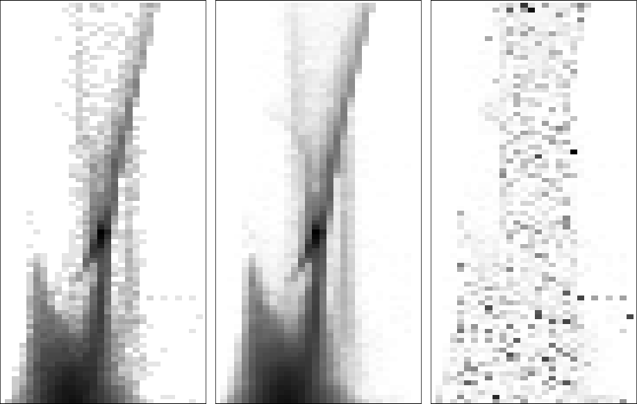 |
Figure 8:
Example of simulated
|
| Open with DEXTER | |
As illustrated in Fig. 7,
the TRILEGAL code can also simulate the synthetic Hess diagram for a
set of partial models, with the advantage of easily generating them in
the UKIDSS photometric system, as well as allowing greater control of all
input parameters involved (see Sect. 2.3).
Therefore we decide to provide these Hess diagrams directly to StarFISH,
using it as a platform for determining the SFRs for our VMC simulated data by
means of a ![]() -like statistics minimisation.
The search for the best solution was done internally in StarFISH by
the amoeba algorithm that used a
downhill strategy to find the minimum
-like statistics minimisation.
The search for the best solution was done internally in StarFISH by
the amoeba algorithm that used a
downhill strategy to find the minimum ![]() -like statistics value.
-like statistics value.
An extra possibility offered by TRILEGAL is the construction of an
additional partial model for the MW foreground ![]() . Indeed, this is done by simulating
the MW population towards the galactic coordinates under examination
for the same total observed area, but averaging over many simulations
so as to reduce the Poisson noise. This partial model is provided to
StarFISH and used in the
. Indeed, this is done by simulating
the MW population towards the galactic coordinates under examination
for the same total observed area, but averaging over many simulations
so as to reduce the Poisson noise. This partial model is provided to
StarFISH and used in the ![]() -like statistics minimisation,
together with those used to describe the MC population.
With this procedure, the MW foreground is taken into account in the
SFH determination, without appealing to the (often risky) procedures
of statistical decontamination based on observating external control
fields. To our knowledge, this is the first time that such a
procedure has been adopted in SFH-recovery work. Once the MW
foreground model is calibrated, its corresponding
-like statistics minimisation,
together with those used to describe the MC population.
With this procedure, the MW foreground is taken into account in the
SFH determination, without appealing to the (often risky) procedures
of statistical decontamination based on observating external control
fields. To our knowledge, this is the first time that such a
procedure has been adopted in SFH-recovery work. Once the MW
foreground model is calibrated, its corresponding ![]() could be set to a fixed value, instead of being included in the
could be set to a fixed value, instead of being included in the
![]() -like statistics minimisation.
-like statistics minimisation.
Figure 7 illustrates the generation of a complete set
of partial models,
covering ages from
![]() to 10.15
(t from 0.10 to 14.13 Gyr) divided into 11 elements with a
width of
to 10.15
(t from 0.10 to 14.13 Gyr) divided into 11 elements with a
width of
![]() each and following
an AMR consistent with the LMC clusters (see the panel d, and
Sect. 2.3). In this figure we have grouped the partial
models into just 6 age ranges (plus the MW foreground one)
to achieve clarity.
What is remarkable in the figure is the high
degree of superposition of the different partial models over the RGB
region of the CMD - except of course for the partial model
corresponding to the MW foreground. The MS region of the CMD, instead,
allows a good visual separation of the different populations over the
entire age range, even after considering the effects of photometric
errors and incompleteness.
each and following
an AMR consistent with the LMC clusters (see the panel d, and
Sect. 2.3). In this figure we have grouped the partial
models into just 6 age ranges (plus the MW foreground one)
to achieve clarity.
What is remarkable in the figure is the high
degree of superposition of the different partial models over the RGB
region of the CMD - except of course for the partial model
corresponding to the MW foreground. The MS region of the CMD, instead,
allows a good visual separation of the different populations over the
entire age range, even after considering the effects of photometric
errors and incompleteness.
4.2 Results: Input vs. output SFR(t)
An example of SFH-recovery is presented in the Hess diagrams of
Fig. 8. The input simulation (left panel) was generated
for a constant SFR(t), for an area equivalent to 1 VIRCAM detector
(
![]() )
inside a region with a stellar density typical for
the LMC disk (
)
inside a region with a stellar density typical for
the LMC disk (
![]() ,
that produces a total number of
stars of
,
that produces a total number of
stars of
![]() ). For this simulation,
StarFISH fits the solution represented in the middle panel. Not
surprisingly, the data-model
). For this simulation,
StarFISH fits the solution represented in the middle panel. Not
surprisingly, the data-model ![]() -like statistics
residuals (right panel) are remarkably evenly distributed across the
Hess diagram.
-like statistics
residuals (right panel) are remarkably evenly distributed across the
Hess diagram.
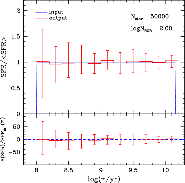 |
Figure 9:
Errors in the recovered SFR(t) in terms of the mean SFR(t) ( top
panel) and input SFR(t) ( bottom panel). The input simulations
correspond to a typical LMC disk region (
|
| Open with DEXTER | |
Figure 9 presents the recovered SFR(t)obtained after performing 100 realisations
for a typical LMC disk region.
As expected, the median SFR(t) over these 100 realisations reproduces the input one remarkably well, with no
indication of systematic errors in the process of
SFH-recovery![]() . The error bars correspond to a
confidence level of 70%, which means that 70% of all individual
realisations are confined within these error bars. Error bars are
almost symmetrical with respect to the expected SFR(t).
Furthermore, errors are typically below 0.4 in units of mean
SFR(t) (top panel), which means uncertainties below 40% (bottom
panel) for almost all ages. The only exception is the youngest age bin,
which presents errors in the SFR that are about two times larger
than those for the intermediate-age stellar populations.
. The error bars correspond to a
confidence level of 70%, which means that 70% of all individual
realisations are confined within these error bars. Error bars are
almost symmetrical with respect to the expected SFR(t).
Furthermore, errors are typically below 0.4 in units of mean
SFR(t) (top panel), which means uncertainties below 40% (bottom
panel) for almost all ages. The only exception is the youngest age bin,
which presents errors in the SFR that are about two times larger
than those for the intermediate-age stellar populations.
There are a many factors that can affect the accuracy of a recovered SFR(t). Among them, the most important are:
- 1.
- the quality of the data in terms of stellar statistics and photometry, which in principle depends (for the same photometric conditions of seeing, exposure times, calibration, etc.) on the density of the field and its covered area in the sky;
- 2.
- the uncertainties in the models themselves, which come from the
possible errors in the adopted input parameters (distance, reddening,
IMF,
,
AMR, etc.), in the stellar evolutionary models,
and in the imperfect reproduction of photometric errors and
completeness;
- 3.
- the incorrect representation of the contamination from other sources, such as foreground MW stars, stars from LMC star clusters, and background galaxies;
- 4.
- the non-uniform properties of the analysed field, like differential reddening or depth in distance.
4.2.1 Random errors for a known AMR
![\begin{figure}
\par\includegraphics[width=8cm,clip]{1111810.eps}
\end{figure}](/articles/aa/full_html/2009/21/aa11118-08/img107.png) |
Figure 10:
Errors in the recovered SFR(t)
for four different stellar densities, from the outer LMC disk
( top-left panel) to the LMC centre ( bottom-right panel).
The thick black solid line corresponds to the median solution found
using
|
| Open with DEXTER | |
To estimate the expected random errors in the SFR(t) for the LMC, we performed controlled experiments similar to the one shown in Figure 9, but covering a wide range of conditions in regard to the stellar statistics and crowding. Figure 10 presents the results for four different levels of density, from the outer LMC disk (top-left panel) to the LMC centre (bottom-right panel), for a number of stars (or area) varying by a factor of 8. As can be seen, these two factors dramatically change the level of accuracy that can be achieved in the recovered SFR(t). An increase in the number of stars reduces the errors whereas an increase in crowding for a fixed number of stars acts in the opposite way.
![\begin{figure}
\par\includegraphics[width=8cm,clip]{1111811.eps}
\end{figure}](/articles/aa/full_html/2009/21/aa11118-08/img108.png) |
Figure 11: Errors in the recovered SFR(t) as a function of covered area and density of stars (different lines) for 4 partial models of different ages ( different panels). |
| Open with DEXTER | |
The errors in the recovered SFR(t) as a function of the covered
area, for all simulated density levels, are shown in
Fig. 11 for partial models of four different
ages, from young (top-left panel) to old ones (bottom-right
panel). Here, a very interesting result can be seen: for stars older
than
![]() (
(![]() Gyr), the curves for
different levels of density are almost superposed, revealing that, for
a fixed area, the accuracy in the recovered SFR(t) is roughly
independent of the level of crowding. It can be understood as a
counterbalanced effect between the loss of stars due to a decrease in
completeness, and the gain of stars due to an increase in
density. Therefore, it seems that the SFR(t) for this wide range in
age can be determined with random errors below 20% if an area of
Gyr), the curves for
different levels of density are almost superposed, revealing that, for
a fixed area, the accuracy in the recovered SFR(t) is roughly
independent of the level of crowding. It can be understood as a
counterbalanced effect between the loss of stars due to a decrease in
completeness, and the gain of stars due to an increase in
density. Therefore, it seems that the SFR(t) for this wide range in
age can be determined with random errors below 20% if an area of
![]() is used. Increasing the area by a factor of four means
that the level of uncertainty drops to below 10%.
is used. Increasing the area by a factor of four means
that the level of uncertainty drops to below 10%.
On the other hand, for partial models younger than
![]() (
(![]() Gyr),
the errors in the recovered SFR(t) are significantly greater
in the less dense regions.
Since stars in this narrow age range are mainly identified in the
upper main sequence at
Gyr),
the errors in the recovered SFR(t) are significantly greater
in the less dense regions.
Since stars in this narrow age range are mainly identified in the
upper main sequence at
![]() and in the core-helium
burning phases at
and in the core-helium
burning phases at
![]() (see Fig. 7),
this effect can be understood by the fact that for these brighter
stars the increase in stellar density is not followed by a significant
decrease in completeness. Indeed, Fig. 4 indicates the
completeness is in general higher than 60% and 90% for
(see Fig. 7),
this effect can be understood by the fact that for these brighter
stars the increase in stellar density is not followed by a significant
decrease in completeness. Indeed, Fig. 4 indicates the
completeness is in general higher than 60% and 90% for
![]() and
and
![]() stars, respectively, for the entire range
of stellar densities of the LMC. In this situation, what determines
the accuracy for a fixed area is simply the number of observed stars,
which is proportional to the density. In particular, our simulations
reveal the lack of stellar statistics in the outermost and less dense
LMC regions, which require large areas to reach a statistically
significant number of young stars. For instance, a level of
uncertainty 20% in the recovered young SFR(t) is obtained for an
area
stars, respectively, for the entire range
of stellar densities of the LMC. In this situation, what determines
the accuracy for a fixed area is simply the number of observed stars,
which is proportional to the density. In particular, our simulations
reveal the lack of stellar statistics in the outermost and less dense
LMC regions, which require large areas to reach a statistically
significant number of young stars. For instance, a level of
uncertainty 20% in the recovered young SFR(t) is obtained for an
area ![]() 10 times larger (
10 times larger (![]()
![]() )
in the periphery of the
LMC than in more central regions.
)
in the periphery of the
LMC than in more central regions.
![\begin{figure}
\par\includegraphics[width=8.8cm,clip]{1111812.eps}
\end{figure}](/articles/aa/full_html/2009/21/aa11118-08/img115.png) |
Figure 12:
Distribution of the fraction of observed stars ( top panel) and its Poisson relative errors ( bottom panel, black lines) as a function of age. These errors correspond to
|
| Open with DEXTER | |
The errors in the SFR(t) were also compared with those expected by
the Poisson statistics in the number of observed stars for each
partial model, as presented by Fig. 12. This figure
reveals that the errors in the SFR(t) can be roughly understood as a
propagation of the Poisson errors by a factor ![]() 10. This explains
why errors are smaller for the older ages, despite the fact that the
different partial models are - due to the adoption of a logarithmic
age scale - roughly uniformly separated in the CMD.
10. This explains
why errors are smaller for the older ages, despite the fact that the
different partial models are - due to the adoption of a logarithmic
age scale - roughly uniformly separated in the CMD.
4.2.2 Random errors for an unknown AMR
![\begin{figure}
\par\includegraphics[width=8cm,clip]{1111813.eps}
\end{figure}](/articles/aa/full_html/2009/21/aa11118-08/img116.png) |
Figure 13: The top panel shows the distribution of metallicities of the partial models adopted in this work: The central solid line is the AMR adopted as a reference, and is used in all of our SFH-recovery experiments. At every age (or age bin), 4 additional partial models (along the dotted lines) can be defined and inserted in the SFH-recovery, then allowing us to access the AMR and its uncertainty (see text for details). The bottom panel shows the difference between the input and output AMRs for the case in which 5 partial models were adopted for each age bin. |
| Open with DEXTER | |
In our previous discussion we naively assumed that the AMR of the LMC is well known, by using a set of partial models that strictly follows the AMR used in the simulations. The real situation is much more complicated. Not only is the AMR not well established, but it also may present significant spreads (for a single age) and vary from place to place over the LMC disk. To face this situation, it is advisable to allow a more flexible approach for the SFH-recovery, in which we have different partial models for every age bin covering a significant range in metallicity.
We adopt the scheme illustrated in the top panel of
Fig. 13; that is, for every age bin, we build
partial models of 5 different metallicities, centred at the [M/H] value given by the reference AMR, and separated by steps of
0.2 dex. This gives a total of 56 partial models, and drastically
increases the CPU time (by a factor of ![]() 100) needed by StarFISH
to converge towards the
100) needed by StarFISH
to converge towards the ![]() -like statistics minimum.
Once the minimum is found, we compute the rj(t)-added SFR(t)and the rj(t)-weighted average
-like statistics minimum.
Once the minimum is found, we compute the rj(t)-added SFR(t)and the rj(t)-weighted average
![]() for each age bin over the five
partial models with different levels of metallicity.
After doing the same for 100 realisations of the input simulation,
we derive the median and the confidence level of 70%
(assumed as the error bar) for the output SFR(t) and
for each age bin over the five
partial models with different levels of metallicity.
After doing the same for 100 realisations of the input simulation,
we derive the median and the confidence level of 70%
(assumed as the error bar) for the output SFR(t) and
![]() .
Figures 13 and
14 illustrate the results for the case of a
constant input SFR(t) and
.
Figures 13 and
14 illustrate the results for the case of a
constant input SFR(t) and
![]() .
.
In the top panel of Fig. 13, the dots with
error bars show the output AMR, which falls remarkably close to the
input one (continuous line). The error bars are smaller than 0.1 dex
at all ages. The bottom panel plots the relative errors in the
derived
![]() ,
showing that they are slightly more significant for
populations of age
,
showing that they are slightly more significant for
populations of age
![]() .
Anyway, the main result
here is that the errors in
.
Anyway, the main result
here is that the errors in
![]() are always smaller than the
0.2 dex separation between the different partial models.
are always smaller than the
0.2 dex separation between the different partial models.
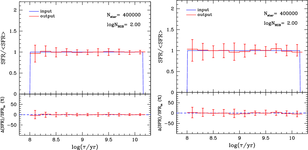 |
Figure 14:
Errors in the recovered SFR(t) in terms of the mean SFR(t) ( top panels) and input SFR(t) ( bottom panels), for a typical LMC disk region inside the area of 8 VIRCAM detector
(
|
| Open with DEXTER | |
Figure 14 instead compares, for the same simulation, the errors in the SFR(t) that result either considering (right panel) or not considering (left panel) the partial models with metallicity different from the reference AMR one. In other words, the left panel shows the SFR(t) that would be recovered if the AMR were known exactly in advance, whereas the right panel shows the SFR(t) for the cases in which the AMR is unknown or, alternatively, is affected by significant observational errors. It can be easily noticed that the SFR(t) is correctly recovered in both cases, although errors in the second case (right panel) are about 2 or 3 times greater than in the first case. Needless to say, the second situation is the more realistic one, and will likely be the one applied in the analysis of VMC data.
4.2.3 Systematic errors related to distance and reddening
Accessing all the systematic errors in the derived SFR(t) is beyond
the scope of this paper; however, the errors associated with the
variations in the distance and reddening are of particular interest
here, since both quantities are expected to vary noticeably across the
LMC, hence having the potential to affect the patterns in the
spacially-resolved SFH. Fortunately, these errors are very easily
accessed with our method, since we know the
![]() and AVvalues of the simulations exactly, as well as those assumed during the
SFH-recovery.
and AVvalues of the simulations exactly, as well as those assumed during the
SFH-recovery.
![\begin{figure}
\par\includegraphics[width=8cm,clip]{1111815.eps}
\end{figure}](/articles/aa/full_html/2009/21/aa11118-08/img122.png) |
Figure 15:
The top panels show the minimum |
| Open with DEXTER | |
The propagation of the uncertainties in the assumed distance modulus
and reddening in the recovered SFR(t) was explored in a series of
control experiments, in which a simulation performed with the
canonical
![]() and
and
![]() was submitted to a series of
SFH-recovery analyses covering a range of
was submitted to a series of
SFH-recovery analyses covering a range of
![]() and
and
![]() .
More
specifically,
.
More
specifically,
![]() was varied from 18.40 to 18.60 and
was varied from 18.40 to 18.60 and
![]() from
0.04 to 0.1. The results of these tests can be seen in
Fig. 15, which presents the effect of wrong
choices on these parameters not only in the recovered SFR(t) (bottom
panel) but also in the minimum value for the
from
0.04 to 0.1. The results of these tests can be seen in
Fig. 15, which presents the effect of wrong
choices on these parameters not only in the recovered SFR(t) (bottom
panel) but also in the minimum value for the
![]() -like statistics (top panels).
-like statistics (top panels).
As expected, the absolute minimum value for the
![]() -like statistics was found
for the synthetic Hess diagrams with the right distance modulus and
reddening. Based on the
-like statistics was found
for the synthetic Hess diagrams with the right distance modulus and
reddening. Based on the ![]() -like statistics dispersion
for 100 simulations, we estimated that the errors in these parameters are about
-like statistics dispersion
for 100 simulations, we estimated that the errors in these parameters are about
![]() mag and
mag and
![]() mag. These errors
also imply systematic errors in the recovered SFR(t) of up to
mag. These errors
also imply systematic errors in the recovered SFR(t) of up to
![]() 30% (Fig. 15, bottom panel).
30% (Fig. 15, bottom panel).
The above experiments clearly suggest us that the mean distance
and reddening should be considered as free parameters in the analysis,
and varied by a few 0.01 mag so that we can identify the best-fitting
values of
![]() and
and
![]() ,
together with the best-fitting SFH. This
kind of procedure has been adopted by e.g. Holtzman et al. (1997) and
Olsen (1999) in their study of small regions over the LMC, and it
is also implemented in the MATCH SFH-recovery package by
Dolphin (2002). Occasionally, one could also consider small spreads
in both
,
together with the best-fitting SFH. This
kind of procedure has been adopted by e.g. Holtzman et al. (1997) and
Olsen (1999) in their study of small regions over the LMC, and it
is also implemented in the MATCH SFH-recovery package by
Dolphin (2002). Occasionally, one could also consider small spreads
in both
![]() and
and
![]() and test whether they improve the
and test whether they improve the
![]() -like statistics minimisation.
Once applied to the entire VMC area, the final
result of this procedure will be independent maps of the geometry and
reddening across the MC system, which can complement those obtained
with other methods.
-like statistics minimisation.
Once applied to the entire VMC area, the final
result of this procedure will be independent maps of the geometry and
reddening across the MC system, which can complement those obtained
with other methods.
5 Concluding remarks
In this paper we have performed detailed simulations of the LMC images expected from the VMC Survey and analysed them in terms of the expected accuracy in determining the space-resolved SFH. Our main conclusions so far are the following:
- 1.
- For a typical
 LMC field of median stellar density, the
random errors in the recovered SFR(t) will typically be smaller than
20% for 0.2 dex-wide age bins.
LMC field of median stellar density, the
random errors in the recovered SFR(t) will typically be smaller than
20% for 0.2 dex-wide age bins.
- 2.
- For all ages over 0.4 Gyr, at increasing stellar densities the better statistics largely compensates for the effects of increased photometric errors and decreased completeness, so that good-quality SFR(t) can be determined even for the most crowded regions in the LMC bar. The SFR(t) errors decrease roughly in proportion to the square of the total number of stars. The exception to this rule regards the youngest stars, which are less affected by incompleteness because of their brightness. In this case, however, the stellar statistics are intrinsically small and large areas are needed to reach the same SFR(t) accuracy as for the intermediate-age and old LMC stars.
- 3.
- Although the AMR [M/H](t) can be recovered with accuracies better than 0.2 dex, the uncertainties in the AMR can significantly affect the quality of the derived SFR(t), increasing their errors by a factor of about 2.5.
- 4.
- The minimisation algorithms allow identification of the best-fitting
reddening and distance with accuracies of the order of 0.02 mag in
distance modulus and 0.01 mag in
 .
.
Another factor to be considered in the final analysis is that for old ages the SFR(t) is expected to vary very smoothly across the LMC, as indicated for instance by Cioni et al. (2000) and Nikolaev & Weinberg (2000). This large-scale correlation in the old SFR(t)may be used as an additional constraint during the SFH-recovery and may help to reduce the errors in the SFR(t) at all ages.
A forthcoming paper will discuss the expected accuracy in more detail over the complete VMC area, including the SMC and this accuracy's dependence on other variables and constraints, which were not discussed in this work (binaries, depth in distance, reddening variations, IMF, etc.). The present work already illustrates the excellent accuracy in the measurements of the space-resolved SFH, which will be made possible by VMC data. Moreover, it demonstrates that detailed SFH-recovery using deep near-infrared photometry is also feasible, as much as it has always been for visual observations.
Acknowledgements
This work is based in part on data obtained as part of the UKIRT Infrared Deep Sky Survey. This publication makes use of data products from the Two Micron All Sky Survey, which is a joint project of the University of Massachusetts and the Infrared Processing and Analysis Center/California Institute of Technology, funded by the National Aeronautics and Space Administration and the National Science Foundation.We acknowledge the referee for useful comments and suggestions that helped us to significantly improve the quality of the paper, especially the discussion about the different methods of recovering the SFH (Sect. 4). We are very grateful to Jim Emerson for providing preliminary VISTA filter throughputs. L.G. acknowledges the inspiring roles of J. Dalcanton, A. Dolphin, J. Harris, J. Holtzman, K. Olsen, and B. Williams (and their papers) in some of the aspects implemented/tested in this work. We acknowledge support from the Brazilian funding agency CNPq, and from INAF/PRIN07 CRA 1.06.10.03.
References
- Alves, D. R. 2004, New Astron. Rev., 48, 659 [NASA ADS] [CrossRef]
- Aparicio, A., Gallart, C., & Bertelli, G. 1997, AJ, 114, 680 [NASA ADS] [CrossRef] (In the text)
- Ardeberg, A., Gustafsson, B., Linde, P., & Nissen, P.-E. 1997, A&A, 322, L13 [NASA ADS]
- Bertelli, G., Mateo, M., Chiosi, C., & Bressan, A. 1992, ApJ, 388, 400 [NASA ADS] [CrossRef]
- Bertelli, G., Bressan, A., Chiosi, C., Fagotto, F., & Nasi, E. 1994, A&AS, 106, 275 [NASA ADS] (In the text)
- Bertin, E., & Arnouts, S. 1996, A&AS, 117, 393 [NASA ADS] [CrossRef] [EDP Sciences] (In the text)
- Besla, G., Kallivayalil, N., Hernquist, L., et al. C. 2007, ApJ, 668, 949 [NASA ADS] [CrossRef]
- Cardelli, J. A., Clayton, G. C., & Mathis, J. S. 1989, ApJ, 345, 245 [NASA ADS] [CrossRef] (In the text)
- Carrera, R., Gallart, C., Hardy, E., Aparicio, A., & Zinn, R. 2008, AJ, 135, 836 [NASA ADS] [CrossRef]
- Chabrier, G. 2001, ApJ, 554, 1274 [NASA ADS] [CrossRef] (In the text)
- Chiosi, E., & Vallenari, A. 2007, A&A, 466, 165 [NASA ADS] [CrossRef] [EDP Sciences]
- Cioni, M.-R. L., Habing, H. J., & Israel, F. P. 2000, A&A, 358, L9 [NASA ADS] (In the text)
- Cioni, M.-R. L., Girardi, L., Marigo, P., & Habing, H. J. 2006a, A&A, 448, 77 [NASA ADS] [CrossRef] [EDP Sciences]
- Cioni, M.-R. L., Girardi, L., Marigo, P., & Habing, H. J. 2006b, A&A, 452, 195 [NASA ADS] [CrossRef] [EDP Sciences]
- Cioni, M.-R. L., Bekki, K., Clementini, G., et al. 2008, Publ. Astron. Soc. Austr., 25, 121 [NASA ADS] [CrossRef] (In the text)
- Clementini, G., Gratton, R., Bragaglia, A., et al. 2003, AJ, 125, 1309 [NASA ADS] [CrossRef]
- Cole, A. A., Tolstoy, E., Gallagher, III, J. S., & Smecker-Hane, T. A. 2005, AJ, 129, 1465 [NASA ADS] [CrossRef]
- Cole, A. A., Skillman, E. D., Tolstoy, E., et al. 2007, ApJ, 659, L17 [NASA ADS] [CrossRef]
- da Silva, L., Girardi, L., Pasquini, L., et al. 2006, A&A, 458, 609 [NASA ADS] [CrossRef] [EDP Sciences]
- Dolphin, A. 1997, New Astron., 2, 397 [NASA ADS] [CrossRef] (In the text)
- Dolphin, A. E. 2002, MNRAS, 332, 91 [NASA ADS] [CrossRef] (In the text)
- Dolphin, A. E., Walker, A. R., Hodge, P. W., et al. 2001, ApJ, 562, 303 [NASA ADS] [CrossRef]
- Dolphin, A. E., Saha, A., Skillman, E. D., et al. 2003, AJ, 126, 187 [NASA ADS] [CrossRef]
- Elson, R. A. W., Gilmore, G. F., & Santiago, B. X. 1997, MNRAS, 289, 157 [NASA ADS]
- Elson, R. A. W., Sigurdsson, S., Davies, M., Hurley, J., & Gilmore, G. 1998, MNRAS, 300, 857 [NASA ADS] [CrossRef] (In the text)
- Ferraro, F. R., Fusi Pecci, F., Tosi, M., & Buonanno, R. 1989, MNRAS, 241, 433 [NASA ADS]
- Foucaud, S., Almaini, O., Smail, I., et al. 2007, MNRAS, 376, L20 [NASA ADS] (In the text)
- Freedman, W. L., Madore, B. F., Gibson, B. K., et al. 2001, ApJ, 553, 47 [NASA ADS] [CrossRef] (In the text)
- Gallagher, J. S., Mould, J. R., de Feijter, E., et al. 1996, ApJ, 466, 732 [NASA ADS] [CrossRef]
- Gallart, C., Aparicio, A., Bertelli, G., & Chiosi, C. 1996a, AJ, 112, 2596 [NASA ADS] [CrossRef]
- Gallart, C., Aparicio, A., & Vilchez, J. M. 1996b, AJ, 112, 1928 [NASA ADS] [CrossRef]
- Gallart, C., Freedman, W. L., Aparicio, A., Bertelli, G., & Chiosi, C. 1999, AJ, 118, 2245 [NASA ADS] [CrossRef]
- Gallart, C., Stetson, P. B., Hardy, E., Pont, F., & Zinn, R. 2004, ApJ, 614, L109 [NASA ADS] [CrossRef]
- Gallart, C., Zoccali, M., & Aparicio, A. 2005, ARA&A, 43, 387 [NASA ADS] [CrossRef] (In the text)
- Gardiner, L. T., & Hatzidimitriou, D. 1992, MNRAS, 257, 195 [NASA ADS]
- Girardi, L., Bressan, A., Bertelli, G., & Chiosi, C. 2000, A&AS, 141, 371 [NASA ADS] [CrossRef] [EDP Sciences] (In the text)
- Girardi, L., Bertelli, G., Bressan, A., et al. 2002, A&A, 391, 195 [NASA ADS] [CrossRef] [EDP Sciences]
- Girardi, L., Groenewegen, M. A. T., Hatziminaoglou, E., & da Costa, L. 2005, A&A, 436, 895 [NASA ADS] [CrossRef] [EDP Sciences] (In the text)
- Girardi, L., Dalcanton, J., Williams, B., et al. & the ANGST/ANGRRR Collaboration 2008, PASP, 120, 583 [NASA ADS] [CrossRef] (In the text)
- Grocholski, A. J., Cole, A. A., Sarajedini, A., Geisler, D., & Smith, V. V. 2006, AJ, 132, 1630 [NASA ADS] [CrossRef]
- Grocholski, A. J., Sarajedini, A., Olsen, K. A. G., Tiede, G. P., & Mancone, C. L. 2007, AJ, 134, 680 [NASA ADS] [CrossRef]
- Gullieuszik, M., Held, E. V., Rizzi, L., et al. 2008, MNRAS, 388, 1185 [NASA ADS] [CrossRef] (In the text)
- Harris, J. 2007a, ApJ, 658, 345 [NASA ADS] [CrossRef]
- Harris, J. 2007b, ApJ, 658, 345 [NASA ADS] [CrossRef] (In the text)
- Harris, J., & Zaritsky, D. 2001, ApJS, 136, 25 [NASA ADS] [CrossRef]
- Harris, J., & Zaritsky, D. 2004, AJ, 127, 1531 [NASA ADS] [CrossRef]
- Harris, J., & Zaritsky, D. 2008, Publ. Astron. Soc. Austr., 25, 116 [NASA ADS] [CrossRef]
- Hernandez, X., Valls-Gabaud, D., & Gilmore, G. 1999, MNRAS, 304, 705 [NASA ADS] [CrossRef]
- Hernandez, X., Gilmore, G., & Valls-Gabaud, D. 2000, MNRAS, 317, 831 [NASA ADS] [CrossRef]
- Hernandez, X., & Valls-Gabaud, D. 2008, MNRAS, 383, 1603 [NASA ADS]
- Hewett, P. C., Warren, S. J., Leggett, S. K., & Hodgkin, S. T. 2006, MNRAS, 367, 454 [NASA ADS] [CrossRef] (In the text)
- Holtzman, J. A., Mould, J. R., Gallagher, III, J. S., et al. 1997, AJ, 113, 656 [NASA ADS] [CrossRef] (In the text)
- Holtzman, J. A., Gallagher, III, J. S., Cole, A. A., et al. 1999, AJ, 118, 2262 [NASA ADS] [CrossRef]
- Imara, N., & Blitz, L. 2007, ApJ, 662, 969 [NASA ADS] [CrossRef]
- Javiel, S. C., Santiago, B. X., & Kerber, L. O. 2005, A&A, 431, 73 [NASA ADS] [CrossRef] [EDP Sciences]
- Jørgensen, B. R., & Lindegren, L. 2005, A&A, 436, 127 [CrossRef] [EDP Sciences]
- Kallivayalil, N., van der Marel, R. P., & Alcock, C. 2006a, ApJ, 652, 1213 [NASA ADS] [CrossRef]
- Kallivayalil, N., van der Marel, R. P., Alcock, C., et al. 2006b, ApJ, 638, 772 [NASA ADS] [CrossRef]
- Kato, D., Nagashima, C., Nagayama, T., et al. 2007, PASJ, 59, 615 [NASA ADS] (In the text)
- Kerber, L. O., Santiago, B. X., & Brocato, E. 2007, A&A, 462, 139 [NASA ADS] [CrossRef] [EDP Sciences]
- Kroupa, P. 2001, MNRAS, 322, 231 [NASA ADS] [CrossRef]
- Kroupa, P. 2002, Science, 295, 82 [NASA ADS] [CrossRef]
- Lawrence, A., Warren, S. J., Almaini, O., et al. 2007, MNRAS, 379, 1599 [NASA ADS] [CrossRef] (In the text)
- Mackey, A. D., & Gilmore, G. F. 2003, MNRAS, 338, 85 [NASA ADS] [CrossRef]
- Marigo, P., & Girardi, L. 2007, A&A, 469, 239 [NASA ADS] [CrossRef] [EDP Sciences] (In the text)
- Marigo, P., Girardi, L., & Chiosi, C. 2003, A&A, 403, 225 [NASA ADS] [CrossRef] [EDP Sciences] (In the text)
- Marigo, P., Girardi, L., Bressan, A., et al. 2008, A&A, 482, 883 [NASA ADS] [CrossRef] [EDP Sciences] (In the text)
- Naylor, T., & Jeffries, R. D. 2006, MNRAS, 373, 1251 [NASA ADS] [CrossRef]
- Nikolaev, S., & Weinberg, M. D. 2000, ApJ, 542, 804 [NASA ADS] [CrossRef]
- Nikolaev, S., Drake, A. J., Keller, S. C., et al. 2004, ApJ, 601, 260 [NASA ADS] [CrossRef]
- Noël, N. E. D., Gallart, C., Costa, E., & Méndez, R. A. 2007, AJ, 133, 2037 [NASA ADS] [CrossRef]
- Nordström, B., Mayor, M., Andersen, J., et al. 2004, A&A, 418, 989 [NASA ADS] [CrossRef] [EDP Sciences]
- Olsen, K. A. G. 1999, AJ, 117, 2244 [NASA ADS] [CrossRef]
- Olszewski, E. W., Schommer, R. A., Suntzeff, N. B., & Harris, H. C. 1991, AJ, 101, 515 [NASA ADS] [CrossRef]
- Piatek, S., Pryor, C., & Olszewski, E. W. 2008, AJ, 135, 1024 [NASA ADS] [CrossRef]
- Schaefer, B. E. 2008, AJ, 135, 112 [NASA ADS] [CrossRef]
- Schlegel, D. J., Finkbeiner, D. P., & Davis, M. 1998, ApJ, 500, 525 [NASA ADS] [CrossRef] (In the text)
- Skillman, E. D., Tolstoy, E., Cole, A. A., et al. 2003, ApJ, 596, 253 [NASA ADS] [CrossRef]
- Smecker-Hane, T. A., Cole, A. A., Gallagher, III, J. S., & Stetson, P. B. 2002, ApJ, 566, 239 [NASA ADS] [CrossRef]
- Stappers, B. W., Mould, J. R., Sebo, K. M., et al. 1997, PASP, 109, 292 [NASA ADS] [CrossRef]
- Stetson, P. B. 1987, PASP, 99, 191 [NASA ADS] [CrossRef] (In the text)
- Subramaniam, A. 2005, A&A, 430, 421 [NASA ADS] [CrossRef] [EDP Sciences]
- Tolstoy, E., & Saha, A. 1996, ApJ, 462, 672 [NASA ADS] [CrossRef]
- Tosi, M., Greggio, L., & Focardi, P. 1989, Ap&SS, 156, 295 [NASA ADS] [CrossRef]
- Tosi, M., Greggio, L., Marconi, G., & Focardi, P. 1991, AJ, 102, 951 [NASA ADS] [CrossRef]
- van der Marel, R. P., & Cioni, M.-R. L. 2001, AJ, 122, 1807 [NASA ADS] [CrossRef]
- van der Marel, R. P., Alves, D. R., Hardy, E., & Suntzeff, N. B. 2002, AJ, 124, 2639 [NASA ADS] [CrossRef]
- Vanhollebeke, E., Groenewegen, M. A. T., & Girardi, L. 2009, ArXiv e-prints, accepted (In the text)
- Vergely, J.-L., Köppen, J., Egret, D., & Bienaymé, O. 2002, A&A, 390, 917 [NASA ADS] [CrossRef] [EDP Sciences]
- Warren, S. J., Hambly, N. C., Dye, S., et al. 2007, MNRAS, 375, 213 [NASA ADS] [CrossRef] (In the text)
- Yuk, I.-S., & Lee, M. G. 2007, ApJ, 668, 876 [NASA ADS] [CrossRef]
- Zaritsky, D., Harris, J., & Thompson, I. 1997, AJ, 114, 1002 [NASA ADS] [CrossRef] (In the text)
- Zaritsky, D., Harris, J., Thompson, I. B., & Grebel, E. K. 2004, AJ, 128, 1606 [NASA ADS] [CrossRef]
Footnotes
- ... System
![[*]](/icons/foot_motif.png)
- See http://www.vista.ac.uk and http://www.star.herts.ac.uk/~mcioni/vmc/ for more information.
- ...
SFH-recovery
- The previous attempts of Cioni et al. (2006b,a) based on
 data, were based on the shallow
observations from DENIS and 2MASS, which are limited to the upper RGB
and above. Consequently, they could access the general trends in the
mean age and metallicity across the MCs, but not the detailed
age-resolved SFH.
data, were based on the shallow
observations from DENIS and 2MASS, which are limited to the upper RGB
and above. Consequently, they could access the general trends in the
mean age and metallicity across the MCs, but not the detailed
age-resolved SFH.
- ... UKIDSS
- Throughout this
paper, we name the 2.2
 m filter as
  when
referring to VISTA, 2MASS and DENIS, and as K when referring to our
simulations and to UKIDSS data. Notice however that, for all practical
purposes, the actual difference between these filters is not a matter
of concern.
when
referring to VISTA, 2MASS and DENIS, and as K when referring to our
simulations and to UKIDSS data. Notice however that, for all practical
purposes, the actual difference between these filters is not a matter
of concern.
- ...Marigo et al. (2008)
- http://stev.oapd.inaf.it/dustyAGB07
- ... IRAF
- IRAF is distributed by the National Optical Astronomy Observatory, which is operated by the Association of Universities for Research in Astronomy (AURA) under cooperative agreement with the National Science Foundation.
- ...
IMF
- With a slope
 for
for
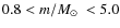 and
and
 for
for
 ,
where the Salpeter slope
is
,
where the Salpeter slope
is
 .
.
- ... 0.7
- This is the mass ratio interval in which the secondary significantly affects the photometry of the system.
- ... magnitudes
- This is of course a crude approximation since deeper surveys sample higher galaxy redshifts. However, it is justified by the lack of deep enough Ydata and by how little impact such faint galaxies have in our stellar photometry (see Sect. 3.2).
- ... code
- Available at http://www.noao.edu/staff/jharris/SFH/
- ... MCPS)
- http://ngala.as.arizona.edu/dennis/mcsurvey.html
- ... foreground
- See http://stev.oapd.inaf.it/trilegal
- ...
SFH-recovery
- As a consequence, the total integral of the SFR is also well recovered.
All Figures
| |
Figure 1:
The area VMC will likely cover in the LMC (solid line) and SMC (dashed line) as a function of the surface density of RGB stars,
|
| Open with DEXTER | |
| In the text | |
| |
Figure 2:
A series of Marigo et al. (2008) isochrones in the UKIDSS photometric system. The figure shows the absolute (MK,
|
| Open with DEXTER | |
| In the text | |
| |
Figure 3:
An image simulation for the area next to the star cluster NGC 1805 (
|
| Open with DEXTER | |
| In the text | |
| |
Figure 4:
Photometric errors ( left panels) and completeness curves ( right panels) in the artificial YJK images for the LMC for different levels of crowding. The thin curves present the results for
the aperture photometry covering the entire expected range of density
of field stars (
|
| Open with DEXTER | |
| In the text | |
| |
Figure 5:
Example of (K,
|
| Open with DEXTER | |
| In the text | |
| |
Figure 6:
A comparison between the aperture photometry
from UKIDSS image data ( left) and the corresponding simulation
( right) for a 0.21
|
| Open with DEXTER | |
| In the text | |
| |
Figure 7:
Simulated
|
| Open with DEXTER | |
| In the text | |
| |
Figure 8:
Example of simulated
|
| Open with DEXTER | |
| In the text | |
| |
Figure 9:
Errors in the recovered SFR(t) in terms of the mean SFR(t) ( top
panel) and input SFR(t) ( bottom panel). The input simulations
correspond to a typical LMC disk region (
|
| Open with DEXTER | |
| In the text | |
| |
Figure 10:
Errors in the recovered SFR(t)
for four different stellar densities, from the outer LMC disk
( top-left panel) to the LMC centre ( bottom-right panel).
The thick black solid line corresponds to the median solution found
using
|
| Open with DEXTER | |
| In the text | |
| |
Figure 11: Errors in the recovered SFR(t) as a function of covered area and density of stars (different lines) for 4 partial models of different ages ( different panels). |
| Open with DEXTER | |
| In the text | |
| |
Figure 12:
Distribution of the fraction of observed stars ( top panel) and its Poisson relative errors ( bottom panel, black lines) as a function of age. These errors correspond to
|
| Open with DEXTER | |
| In the text | |
| |
Figure 13: The top panel shows the distribution of metallicities of the partial models adopted in this work: The central solid line is the AMR adopted as a reference, and is used in all of our SFH-recovery experiments. At every age (or age bin), 4 additional partial models (along the dotted lines) can be defined and inserted in the SFH-recovery, then allowing us to access the AMR and its uncertainty (see text for details). The bottom panel shows the difference between the input and output AMRs for the case in which 5 partial models were adopted for each age bin. |
| Open with DEXTER | |
| In the text | |
| |
Figure 14:
Errors in the recovered SFR(t) in terms of the mean SFR(t) ( top panels) and input SFR(t) ( bottom panels), for a typical LMC disk region inside the area of 8 VIRCAM detector
(
|
| Open with DEXTER | |
| In the text | |
| |
Figure 15:
The top panels show the minimum |
| Open with DEXTER | |
| In the text | |
Copyright ESO 2009
Current usage metrics show cumulative count of Article Views (full-text article views including HTML views, PDF and ePub downloads, according to the available data) and Abstracts Views on Vision4Press platform.
Data correspond to usage on the plateform after 2015. The current usage metrics is available 48-96 hours after online publication and is updated daily on week days.
Initial download of the metrics may take a while.