| Issue |
A&A
Volume 499, Number 3, June I 2009
|
|
|---|---|---|
| Page(s) | 905 - 916 | |
| Section | The Sun | |
| DOI | https://doi.org/10.1051/0004-6361/200810844 | |
| Published online | 25 March 2009 | |
Morphology and density structure of post-CME current sheets
B. Vrsnak1 - G. Poletto2 - E. Vujic3 - A. Vourlidas4 - Y.-K. Ko4 - J. C. Raymond5 - A. Ciaravella6 - T. Zic1 - D. F. Webb7 - A. Bemporad8 - F. Landini9 - G. Schettino9 - C. Jacobs10 - S. T. Suess11
1 - Hvar Observatory, Faculty of Geodesy, Zagreb, Croatia
2 - INAF-Arcetri Observatory, Firenze, Italy
3 - Faculty of Science, Geophysical Department, Croatia
4 - Naval Research Laboratory, Washington DC, USA
5 - Harvard-Smithsonian Center for Astrophysics, Cambridge, USA
6 - INAF-Palermo Observatory, Palermo, Italy
7 - Boston College and AFRL, Hanscom, USA
8 - INAF-Torino Astrophysical Observatory, Pino Torinese, Italy
9 - Dept. of Astronomy and Space Science, University of Florence, Italy
10 - Centrum voor Plasma-Astrofysica, K. U. Leuven, Belgium
11 - NASA Marshall Space Flight Center, Huntsville, USA
Received 22 August 2008 / Accepted 6 February 2009
Abstract
Context. Eruption of a coronal mass ejection (CME) drags and ``opens'' the coronal magnetic field, presumably leading to the formation of a large-scale current sheet and field relaxation by magnetic reconnection.
Aims. We analyze the physical characteristics of ray-like coronal features formed in the aftermath of CMEs, to confirm whether interpreting this phenomenon in terms of a reconnecting current sheet is consistent with observations.
Methods. The study focuses on measurements of the ray width, density excess, and coronal velocity field as a function of the radial distance.
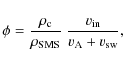
Results. The morphology of the rays implies that they are produced by Petschek-like reconnection in the large-scale current sheet formed in the wake of CME. The hypothesis is supported by the flow pattern, often showing outflows along the ray, and sometimes also inflows into the ray. The inferred inflow velocities range from 3 to 30 km s-1, and are consistent with the narrow opening-angle of rays, which add up to a few degrees. The density of rays is an order of magnitude higher than in the ambient corona. The density-excess measurements are compared with the results of the analytical model in which the Petschek-like reconnection geometry is applied to the vertical current sheet, taking into account the decrease in the external coronal density and magnetic field with height.
Conclusions. The model results are consistent with the observations, revealing that the main cause of the density excess in rays is a transport of the dense plasma from lower to higher heights by the reconnection outflow.
Key words: Sun: coronal mass ejections (CMEs) - Sun: corona - Sun: solar wind - magnetohydrodynamics (MHD)
1 Introduction
According to our current understanding of solar coronal mass ejections (CMEs), the eruption of an unstable magnetic structure is closely associated with the formation of a large-scale current sheet (hereinafter CS) in the wake of the eruption. This concept was initially proposed and developed by Carmichael (1964), Sturrock (1966), Hirayama (1974), and Kopp & Pneuman (1976), connecting the large-scale eruption and the localized energy release in the form of flare (the so-called CSHKP model). When the current sheet becomes long enough, the tearing instability sets in, leading to fast reconnection of magnetic field (for the analytical, numerical, laboratory, and observational results, see, e.g., Furth et al. 1963; Ugai 1987; Gekelman & Pfister 1988; and Vrsnak et al. 2003, respectively). Reconnection in the post-CME current sheet results in an abrupt energy release causing a flare, and also enhances and prolongs the acceleration of the erupting magnetic field structure (e.g., Lin 2004; Vrsnak 2008, and references therein). Numerical MHD simulations covering various scales, from the low corona to 1 AU, also demonstrated post-CME current sheet formation, clearly revealing the importance of the reconnection in the initiation, acceleration, and propagation of CMEs (see, e.g., Riley et al. 2002; Roussev et al. 2003; Török et al. 2004; and Riley et al. 2007; and for a review, see Forbes et al. 2006).
The most prominent consequence of CME-associated reconnection is the appearance of the so-called two-ribbon flare, which is closely related to the CME acceleration stage (e.g., Maricic et al. 2007, and references therein). The ribbon expansion away from the magnetic inversion line, associated with a growing system of hot loops connecting the ribbons, has led to the formulation of the CSHKP model. The discovery of cusped structure above the flare loops (e.g., Tsuneta et al. 1992; Forbes & Acton 1996; Tsuneta 1996), loop-top hard X-ray sources (e.g., Masuda et al. 1994; Aschwanden et al. 1996; Sui et al. 2004; Veronig et al. 2006), the loop shrinkage (e.g., Svestka et al. 1987; Forbes & Acton 1996; Sheeley et al. 2004; Vrsnak et al. 2006), and the recognition of growing post-eruption loop systems in the absence of flares, all provided further support of the CSHKP scenario. Additional evidence of reconnection below the erupting flux-rope may be found in the so-called disconnection events (e.g., Webb & Cliver 1995; Simnett et al. 1997; Wang et al. 1999), downflows above the post-eruption arcades (e.g., McKenzie & Hudson 1999; Innes et al. 2003a; Asai et al. 2004), horizontal converging flows above the loops (Yokoyama et al. 2001; Lin et al. 2005), and flare-associated radio emission below the eruptive prominence (Vrsnak et al. 2003).
Post-CME features detectable in UV spectra (Innes et al. 2003b; Bemporad et al. 2006; Lin et al. 2005; Ko et al. 2003; Ciaravella & Raymond 2008; Ciaravella et al. 2002), X-ray images (Sui et al. 2005,2004), and white light coronagraph images (Lin et al. 2005; Ko et al. 2003; Webb et al. 2003) have been attributed to the current sheets expected to ``connect'' the flare loops to the CME core. The UV spectral signature is generally emission in the high temperature lines of Fe XVIII or Fe XIX formed at 5-10 MK. EUV images from the Extreme-ultraviolet Imaging Telescope (EIT) onboard the Solar and Heliospheric Observatory (SoHO) and the Transition Region and Coronal Explorer (TRACE) show emission in Fe XXIV at even higher temperatures (Innes et al. 2003a; McKenzie & Hudson 1999). The UV features decay slowly, on timescales of between several hours (Ciaravella & Raymond 2008) and a few days (Bemporad et al. 2006; Ko et al. 2003). The X-ray data from the Reuven Ramaty High Energy Solar Spectroscopic Imager (RHESSI) exhibit regions of high temperature emission above loop tops, and both the morphology at different energies and the evolution of the structures are consistent with the CS indentification. The white light features are bright, narrow rays that appear to connect the cusped flaring loop system to the CME core (Lin et al. 2005). Some show blobs of plasma moving outwards at several hundred km s-1. Like the UV features, the white-light structures can last for a day or two. In general, white light observations reveal the electron column density, UV data constrain temperatures, emission measures, and Doppler shifts, and X-ray observations reveal very high temperature plasma.
The aim of this paper is to demonstrate that post-CME rays appear as a consequence of the reconnection in the current sheet formed in the wake of CME, and to quantify their basic physical characteristics. We outline the working hypothesis in Sect. 2, and provide details of the model used to compare the theoretical expectations with observations in the Appendix. We present in Sect. 3 our observations and measurements, focusing on the morphology and plasma densities in post-CME rays. The temperature structure and the ionization state will be presented in a separate paper. Our density measurements are compared with the model estimates and some previous empirical results in Sect. 4. Results are discussed and conclusions drawn in Sect. 5.
2 Working hypothesis
![\begin{figure}
\par\includegraphics[width=8.5cm,clip]{0844fig1.eps}
\end{figure}](/articles/aa/full_html/2009/21/aa10844-08/img10.png) |
Figure 1:
a) Interpretation of the ray in terms of the Petschek (1964) reconnection model: DR - diffusion region; SMS - slow mode shocks (dashed lines intersecting at DR); PEL - post-eruption loops. Magnetic field-lines are drawn by thin lines; gray area between the SMSs outlines the post-CME ray. The coordinate system is indicated (the line of sight is in y-direction). b) An element of bifurcated current sheet; arrows mark plasma flows (
|
| Open with DEXTER | |
Since post-CME rays extend outward from cusped structures associated with growing post-eruption loop-systems, our working hypothesis is that they appear as a consequence of the reconnection in the CS formed in the wake of CME. Furthermore, we assume that the reconnection process can be described approximately in terms of the steady-state Petschek regime (Petschek 1964). In this regime, the reconnection takes place within a small diffusion region (DR), from which two pairs of standing slow-mode shocks (SMSs) extend along the axis of symmetry. Thus, the CS is bifurcated, SMSs separating the inflow and outflow region (Petschek 1964; Soward & Priest 1982). At SMSs, the inflowing plasma is compressed, heated, and accelerated, forming the upward and downward reconnection jet (Fig. 1). We note that electric currents are concentrated only in DR and SMSs.
When reconnection occurs in the homogeneous environment, the characteristics of outflowing plasma are determined primarily by the external plasma-to-magnetic pressure ratio, whereas the outflow speed is approximately equal to the external Alfvén speed (see Appendix in Aurass et al. 2002; and Skender et al. 2003). However, in the case of a vertical current sheet, the ambient coronal density and magnetic field decrease with height, so the characteristics of the reconnection jets also depend on height. The main effect is transport of the dense plasma from lower heights upward, which makes the outflow jet far denser than the ambient corona (see Appendix). In this respect, the post-CME ray should be similar to coronal streamers.
Bearing in mind the geometry of the Petschek-type reconnection, the post-CME CS should have distinctive morphological characteristics. It should be thinnest at the height of the diffusion region, and become wider with increasing height. In the homogeneous plasma, the angle between the SMSs is determined by the inflow Mach number (Vrsnak & Skender 2005; Soward & Priest 1982), the half-angle typically equaling a several degrees (Vrsnak & Skender 2005). Thus, for the CS length of several solar radii, the Petschek-CS thickness (the distance between the SMSs) is on the order of 100 Mm. We note that in the case of the vertical CS in the solar corona, where the magnetic field diverges radially, the angle between SMSs should increase with height even at uniform inflow Mach number (see Appendix), so the CS thickness should be somewhat larger than in the plane-symmetric case.
Further important characteristics of the post-CME CSs that determine their appearance in
coronagraphic images, are the horizontal length and the orientation with respect to the line of
sight (Fig. 2). We note that the angle ![]() between the plane of CS and the line of
sight (LoS) must be rather small, otherwise the CS would not appear as a distinct feature in
coronagraphic images. This causes a ``selection effect'', which can explain the fact that post-CME
rays can be recognized only in a relatively small fraction of events (Webb et al. 2003).
between the plane of CS and the line of
sight (LoS) must be rather small, otherwise the CS would not appear as a distinct feature in
coronagraphic images. This causes a ``selection effect'', which can explain the fact that post-CME
rays can be recognized only in a relatively small fraction of events (Webb et al. 2003).
In Fig. 2a, we depict how the effective thickness D of the ray depends on the CS thickness
2d, horizontal length L, and the angle ![]() .
On average, a ray should be thinner and
brighter for smaller
.
On average, a ray should be thinner and
brighter for smaller ![]() (larger LoS column-length
(larger LoS column-length ![]() ). In Fig. 2b, we
illustrate how the variation in
). In Fig. 2b, we
illustrate how the variation in ![]() along the LoS can account for the complex appearance of
the ray (see also Saez et al. 2007), i.e., a wavy CS would be seen by observer as a ``multi-ray''
structure. We note that the angle
along the LoS can account for the complex appearance of
the ray (see also Saez et al. 2007), i.e., a wavy CS would be seen by observer as a ``multi-ray''
structure. We note that the angle ![]() ,
or its variation along the LoS, can vary with both time
and height, such that the morphology of the structure can change with time and can differ at
different heights.
,
or its variation along the LoS, can vary with both time
and height, such that the morphology of the structure can change with time and can differ at
different heights.
![\begin{figure}
\par\includegraphics[width=7cm,clip]{0844fig2.eps}
\end{figure}](/articles/aa/full_html/2009/21/aa10844-08/img11.png) |
Figure 2:
Dependence of the width and morphology of the ray at a given height on the orientation/geometry of the current sheet: a) straight CS; b) wavy CS. The CS half-thickness is denoted by d, horizontal length (i.e., the length in xy-plane, see also Fig. 1) by L, the ray width by D, and the inclination to the line of sight (LoS) by |
| Open with DEXTER | |
3 Observations
3.1 SoHO/LASCO mass images
To analyze the morphology and column density of post-CME rays, we employ data provided by the Large
Angle Spectroscopic Coronagraph (LASCO, Brueckner et al. 1995) onboard SoHO. We focus on the
LASCO-C2 images, which cover radial distances from 2 to 6 solar radii (![]() ). We use, in
particular, the so-called mass images derived from LASCO base-difference images calibrated in units
of solar brightness. These images exhibit changes in the column mass along the line of sight under
the assumption that the structure is in the plane of sky (for details we refer to
Billings 1966; Poland et al. 1981; Vourlidas et al.
2000; and Vourlidas et al. 2002); bright pixels (positive
values) represent areas where the column mass has increased, whereas dark pixels (negative values)
show depleted regions.
). We use, in
particular, the so-called mass images derived from LASCO base-difference images calibrated in units
of solar brightness. These images exhibit changes in the column mass along the line of sight under
the assumption that the structure is in the plane of sky (for details we refer to
Billings 1966; Poland et al. 1981; Vourlidas et al.
2000; and Vourlidas et al. 2002); bright pixels (positive
values) represent areas where the column mass has increased, whereas dark pixels (negative values)
show depleted regions.
We initially considered eleven post-CME ray events, which were spotted while analyzing the associated CMEs for other purposes, i.e., the rays were chosen rather randomly. Thus, no attempt was made to analyze the occurrence rate of post-CME rays (for the criteria and statistical background we refer the reader to Webb et al. 2003). Nevertheless, we note that ray-like features in the wake of CMEs are not uncommon, in particular when considering the specific circumstances under which a post-CME current sheet could be observed: i.e., the level of post-CME activity should not be too high, and the current sheet must be oriented at a small angle with respect to the line of sight and should be relatively stable.
Inspecting the selected sample, we noted intermittent activity in most of the rays, which manifests itself as changes in their shape, contrast, and inclination. These variations were either caused by coronal disturbances originating in remote eruptions, or were indicative of internal activity, such as blob formation/ejection and/or outward propagating wave-like perturbations.
For a detailed analysis, we chose three post-CME rays, observed on 8-9 January 2002, 18 November 2003, and 26 June 2005. The events of 18 November 2003 and 26 June 2005 were selected as examples of relatively stable rays. In both events, we analyzed only one ray image (at 12:50 UT and 06:30 UT, respectively). On the other hand, the event of 8-9 January 2002 did exhibit significant activity, similar to that in the remaining eight events. This event was selected to quantify the level of variability in post-CME rays, and we therefore performed measurements at three different times (00:06, 06:06, and 12:06 UT). We note that the rays in the selected exposures did not have significant blob-like features or similar inhomogeneities, although they might have been present at earlier and/or later times.
3.2 The ray morphology
![\begin{figure}
\par\includegraphics[width=9cm,clip]{0844fig3.eps}
\end{figure}](/articles/aa/full_html/2009/21/aa10844-08/img13.png) |
Figure 3:
a) Simple post-CME ray (9 January 2002 at 06:06 UT); b) complex ray consisting of three radial substructures (9 January 2002 at 02:30 UT). The ray is marked by white arrow. The scale of the LASCO-C2 images is given in pixels (1 pixel corresponds to 11.9 arcsec). The column-mass profiles measured along the bin marked by white lines are shown in the right-hand panels (abscissa scale in pixels). Estimates of the ray width, D, and column-mass excess, |
| Open with DEXTER | |
In Fig. 3, we illustrate the variability in the ray morphology by showing two images of the ray that became recognizable a few hours after the east-limb CME eruption on 8 January 2002 (the first appearance in LASCO-C2 at 17:54 UT). In Fig. 3a, we first show a simple ray pattern that was recorded half a day after the eruption. Four hours earlier, the ray had a complex form consisting of three radial substructures (Fig. 3b); this ``multi-ray'' pattern could be caused by a wavy current sheet, as illustrated in Fig. 2b. Morphological changes of this kind, which develop on timescales of hours are a common characteristic of post-CME rays, since they were present in nine of the eleven events in our initial sample.
Our estimates of the ray width and column-mass excess are based on the LASCO-C2 mass-images
(Fig. 3 left), which for each pixel, provide the difference ![]() between the
column-mass in the actual image and the reference image. In the right-hand panels of Fig. 3,
we show two mass-difference profiles
between the
column-mass in the actual image and the reference image. In the right-hand panels of Fig. 3,
we show two mass-difference profiles
![]() ,
where
,
where ![]() is expressed in g/pixel, while
the abscissa, corresponding to the y coordinate of the LASCO images, is represented in pixels.
The profiles shown were measured in the LASCO-C2 difference-images along the bin marked by white
lines in the left panel of Fig. 3, i.e., roughly perpendicular to the ray direction. The bin
is 10 pixels wide, and the profile shows
is expressed in g/pixel, while
the abscissa, corresponding to the y coordinate of the LASCO images, is represented in pixels.
The profiles shown were measured in the LASCO-C2 difference-images along the bin marked by white
lines in the left panel of Fig. 3, i.e., roughly perpendicular to the ray direction. The bin
is 10 pixels wide, and the profile shows ![]() averaged over the bin width. Pixels with
averaged over the bin width. Pixels with
![]() represent areas where the column-mass remained the same as it was in the reference
image. We note that the mass aside the rays is depleted (
represent areas where the column-mass remained the same as it was in the reference
image. We note that the mass aside the rays is depleted (
![]() ), probably due to the
CME-associated coronal expansion, usually seen as coronal dimming when the eruption is launched
from regions on the solar disc. The depletion might also be caused partly by the presumed inflow
into the current sheet.
), probably due to the
CME-associated coronal expansion, usually seen as coronal dimming when the eruption is launched
from regions on the solar disc. The depletion might also be caused partly by the presumed inflow
into the current sheet.
Given the working hypothesis, where the ray is assumed to be the reconnection outflow jet of a
large-scale Petschek-like bifurcated current sheet, we are interested in the column-mass excess of
the ray, ![]() ,
defined as the difference between the peak in the ray column-mass
,
defined as the difference between the peak in the ray column-mass
![]() and the column-mass in the adjacent corona
and the column-mass in the adjacent corona
![]() .
In other words,
.
In other words, ![]() determines the difference of column-mass associated with the current sheet and the inflow region (
determines the difference of column-mass associated with the current sheet and the inflow region (
![]() ;
see the right-hand panel of Fig. 3a). The ray width D is measured as the full width of the ray structure in the mass-difference profile (Fig. 3a right). The main source of error in estimating
;
see the right-hand panel of Fig. 3a). The ray width D is measured as the full width of the ray structure in the mass-difference profile (Fig. 3a right). The main source of error in estimating ![]() and D is the determination of the value
and D is the determination of the value
![]() ,
since this value is frequently different on opposite sides of the ray (Fig. 3a right). Thus, we estimated the upper and lower limit (dashed arrows in Fig. 3a right), and these
measurements provided us with the error bars plotted in Fig. 4.
,
since this value is frequently different on opposite sides of the ray (Fig. 3a right). Thus, we estimated the upper and lower limit (dashed arrows in Fig. 3a right), and these
measurements provided us with the error bars plotted in Fig. 4.
The measurements illustrated in Fig. 3 were performed on five images of post-CME rays for
the LASCO-C2 range of heights to estimate the radial dependence of the relevant ray parameters. The
measured rays are marked in the mass-images shown in the left column of Fig. 4 (hereinafter
denoted as rays a-e). In the second column of Fig. 4, the ray widths, expressed in
units of the solar radius ![]() ,
are presented as a function of the radial distance, D(R),
where
,
are presented as a function of the radial distance, D(R),
where
![]() .
The ray in Fig. 4a is characterized by a ``multi-ray'' structure, and
we therefore measured only the central feature, which was the most prominent element of the
structure.
.
The ray in Fig. 4a is characterized by a ``multi-ray'' structure, and
we therefore measured only the central feature, which was the most prominent element of the
structure.
Inspecting the graphs, one finds that in the distance range of R=2-2.5 the widths vary
between 0.1 and 0.4 ![]() (mean value 0.26). In the range R=5-6, the widths increase
to 0.4-0.9
(mean value 0.26). In the range R=5-6, the widths increase
to 0.4-0.9 ![]() (mean 0.7). The widths that we found at
(mean 0.7). The widths that we found at ![]() are more than twice as
large as those found by Webb et al. (2003), who analyzed the coronagraph data obtained by the Solar
Maximum Mission (SMM): converting their values of the width expressed in degrees, into units of the
solar radius at the corresponding heights, we find that the mean width reported by Webb et al. (2003, see
Tables 2 and 3 therein) is 0.09
are more than twice as
large as those found by Webb et al. (2003), who analyzed the coronagraph data obtained by the Solar
Maximum Mission (SMM): converting their values of the width expressed in degrees, into units of the
solar radius at the corresponding heights, we find that the mean width reported by Webb et al. (2003, see
Tables 2 and 3 therein) is 0.09 ![]() in this height range. The difference may be
related to the lower sensitivity of SMM.
in this height range. The difference may be
related to the lower sensitivity of SMM.
3.3 The ray density
In the third column of Fig. 4, we show the radial dependencies of column-mass excesses
![]() ,
expressed in g/pixel. Inspecting the graphs
,
expressed in g/pixel. Inspecting the graphs
![]() ,
we find that the slopes
of the fitted power-law functions range from -2.1 to -3.2, the average value being
,
we find that the slopes
of the fitted power-law functions range from -2.1 to -3.2, the average value being
![]() .
.
The column-mass excess ![]() was converted to the number-density excess
was converted to the number-density excess ![]() by assuming
that, due to the spherical geometry, the column length increases in proportion to the radial
distance,
by assuming
that, due to the spherical geometry, the column length increases in proportion to the radial
distance,
![]() .
In particular, we used
.
In particular, we used
![]() Mm at
R=R0=2.16 (the lowest
height of measurements). The outcome is presented in log-log graphs in the fourth column of
Fig. 4, together with the power-law fits. We note that some other choice of
Mm at
R=R0=2.16 (the lowest
height of measurements). The outcome is presented in log-log graphs in the fourth column of
Fig. 4, together with the power-law fits. We note that some other choice of ![]() would shift vertically the
would shift vertically the
![]() dependence, without changing the slope in a log-log graph.
The slope would change only if some other radial dependence
dependence, without changing the slope in a log-log graph.
The slope would change only if some other radial dependence
![]() existed, e.g., the angle
existed, e.g., the angle
![]() was height-dependent.
was height-dependent.
Inspecting the graphs
![]() in Fig. 4, we find that the slopes of the fitted
power-law functions range from -3.1 to -4.2, the average value being
in Fig. 4, we find that the slopes of the fitted
power-law functions range from -3.1 to -4.2, the average value being
![]() .
We pay
special attention to the slope of the fit, since it does not depend on the presumed value of
.
We pay
special attention to the slope of the fit, since it does not depend on the presumed value of
![]() ,
so it can be compared directly with the model results (Sect. 4.1). In this respect it
is important to note that in the case of the smallest slope in the sample, the ray width becomes
approximately constant beyond
,
so it can be compared directly with the model results (Sect. 4.1). In this respect it
is important to note that in the case of the smallest slope in the sample, the ray width becomes
approximately constant beyond
![]() ,
indicating a possible decrease in
,
indicating a possible decrease in ![]() with the
height, i.e., an increase in
with the
height, i.e., an increase in ![]() .
This would imply that in this case the densities are
overestimated at larger heights, since
.
This would imply that in this case the densities are
overestimated at larger heights, since
![]() ,
i.e., the true slope of
,
i.e., the true slope of
![]() is probably steeper.
is probably steeper.
![\begin{figure}
\par\includegraphics[width=18cm,clip]{0844fig4.eps}
\end{figure}](/articles/aa/full_html/2009/21/aa10844-08/img34.png) |
Figure 4: The five measured post-CME rays (indicated by arrows in the full-resolution LASCO-C2 images shown in the first column): a- c) 9 January 2002 at 00:06, 06:06, and 12:06 UT, respectively; d) 18 November 2003 at 12:50 UT; e) 26 June 2005 at 06:30 UT. In the second, third, and fourth column we show the ray width, column-mass excess, and the density excess, as a function of the radial distance. The widths and radial distances are expressed in units of the solar radius. The least-square fits are shown in the insets, together with the correlation coefficient C. |
| Open with DEXTER | |
Since the evaluation of the density excess depends on the choice of the column length ![]() ,
in
Fig. 5 we present an estimate of the number of electrons per unit length of the ray, which
is a parameter independent of
,
in
Fig. 5 we present an estimate of the number of electrons per unit length of the ray, which
is a parameter independent of ![]() .
If we approximate the mass-difference profiles across the
ray by triangular profiles, the mass-excess per unit length of the profile amounts to
.
If we approximate the mass-difference profiles across the
ray by triangular profiles, the mass-excess per unit length of the profile amounts to
![]() ,
from which we evaluate the electron-number excess per unit length of the ray,
,
from which we evaluate the electron-number excess per unit length of the ray, ![]() .
.
Inspecting Fig. 5a, where
![]() is presented separately for all five rays from
Fig. 4, we find that
is presented separately for all five rays from
Fig. 4, we find that
![]() either decreases (rays [a], [b], and [d]) or stays roughly constant (rays [c] and [e]). When averaged, the data from Fig. 5b show a dependence similar to that obtained by Ciaravella & Raymond (2008), who found that after a decrease at low heights, the value of
either decreases (rays [a], [b], and [d]) or stays roughly constant (rays [c] and [e]). When averaged, the data from Fig. 5b show a dependence similar to that obtained by Ciaravella & Raymond (2008), who found that after a decrease at low heights, the value of ![]() becomes approximately constant. Comparing their Fig. 8 with our Fig. 5b, we find that the numbers and trends are similar. However, the radial distance at which
becomes approximately constant. Comparing their Fig. 8 with our Fig. 5b, we find that the numbers and trends are similar. However, the radial distance at which
![]() becomes constant, differs: according to results by Ciaravella & Raymond (2008), this occurs at
becomes constant, differs: according to results by Ciaravella & Raymond (2008), this occurs at
![]() ,
whereas in our case the transition occurs at
,
whereas in our case the transition occurs at
![]() .
In Fig. 5b, we also present the power-law fit, showing that the overall trend could also be described by
.
In Fig. 5b, we also present the power-law fit, showing that the overall trend could also be described by
![]() .
.
3.4 Coronal flows
![\begin{figure}
\par\includegraphics[width=9cm,clip]{0844fig5.eps}
\end{figure}](/articles/aa/full_html/2009/21/aa10844-08/img40.png) |
Figure 5:
Number of electrons per unit length of the ray,
|
| Open with DEXTER | |
Coronal regions beneath CMEs are generally characterized by highly dynamical intricate structures, revealing complex magnetoplasma flows and waves. Consequently, it is difficult to identify persistent systematic flow patterns, especially during periods of increased solar activity, when disturbances from other CMEs affect the coronal region of interest. This also holds for flow patterns associated with post-CME rays, whose morphologies are permanently changing and are strongly affected by disturbances from distant CMEs.
In certain situations, some characteristic flows could however be identified. Most frequently, outward-moving inhomogeneities along the ray are observed, usually having velocities of several hundred km s-1 (e.g., Ko et al. 2003; Lin et al. 2005). Such motions are often interpreted in terms of the reconnection outflow, which may or may not be characterized by the Alfvénic speed (for a discussion we refer to Bárta et al. 2008, and references therein). In this respect, we note that signatures of shrinking loops are also observed occasionaly in the wake of CMEs (e.g., Sheeley & Wang 2002; Sheeley et al. 2004; Sheeley & Wang 2007, and references therein) consistent with decelerated reconnection downflows.
Compared to reconnection outflows, detecting signatures of reconnection inflows is far more
difficult. A possible example was reported by Yokoyama et al. (2001), based on the observations by the
EIT/SoHO. Another example was presented by Lin et al. (2005), who employed data from EIT and the
UltraViolet Coronagraph Spectrometer (UVCS) onboard SoHO. Recently, Bemporad et al. (2008) reported a
``side-reconnection'' in the aftermath of a CME, induced by the CME expansion: from the detection of
two converging reconnecting features at 1.7 ![]() (probably the CME flank and the streamer
boundary), the authors inferred an inflow speed of 3-4 km s-1, close to the 5 km s-1 derived by
Yokoyama et al. (2001).
(probably the CME flank and the streamer
boundary), the authors inferred an inflow speed of 3-4 km s-1, close to the 5 km s-1 derived by
Yokoyama et al. (2001).
In Fig. 6, we present a stack-plot showing an example of the reconnection-inflow pattern observed above the west limb on 8 January 2002 in the LASCO-C2 field-of-view. We note that this post-CME feature is not the ray of 8-9 January 2002 presented in Figs. 3 and 4, which was on the opposite side of the solar disc. This west-limb event was not observed by UVCS, i.e., we do not know if it exhibited Fe XVIII emission, which is one of the criteria for identifying post-CME current sheets. We note that we could not detect a distinctive signature of reconnection inflow in the three post-CME rays analyzed in Sects. 3.2. and 3.3. In these events, no suitable inhomogeneities could be identified to provide tracing of plasma motion in the inflow region (to be discussed in Sect. 5).
The west-limb ray presented in Fig. 6, formed after a faint ejection that was first observed
in LASCO-C2 at 02:54 UT on 8 January 2002 (not listed in the LASCO CME catalog). Each stack
represents the cut along a line parallel to the y-axis of a given LASCO-C2 512![]() 512-pixel
running-difference image, showing the pixel-intensities in the range
x=3.30-3.38
512-pixel
running-difference image, showing the pixel-intensities in the range
x=3.30-3.38 ![]() .
We note that the ray was oriented close to the x-axis of LASCO
images, i.e., the stacks are roughly perpendicular to the ray direction. The stack-plot contains
all images recorded on 8 January 2002 (denoted by an ordinal number on the x-axis of the
stack-plot; the time cadence is on average 24 min).
.
We note that the ray was oriented close to the x-axis of LASCO
images, i.e., the stacks are roughly perpendicular to the ray direction. The stack-plot contains
all images recorded on 8 January 2002 (denoted by an ordinal number on the x-axis of the
stack-plot; the time cadence is on average 24 min).
![\begin{figure}
\par\includegraphics[width=9cm,clip]{0844fig6.eps}
\end{figure}](/articles/aa/full_html/2009/21/aa10844-08/img43.png) |
Figure 6:
a) LASCO-C2 running-difference images of the west-limb ray of 8 January 2002 (13:54 UT), revealing the inflow into the ray. The slice used in the stack-plot shown in b) is outlined by white rectangle centered at
|
| Open with DEXTER | |
The black/white stripes converging towards the ray location, located at
![]() ,
clearly show inflows into the ray. The corresponding velocities in the left
part of the stack-plot are found in the range 15-25 km s-1 (mean
,
clearly show inflows into the ray. The corresponding velocities in the left
part of the stack-plot are found in the range 15-25 km s-1 (mean ![]() km s-1).
These velocities are several times higher than 5 km s-1 reported by Yokoyama et al. (2001). After the slice No. 50 (18:54 UT), the stack-plot shows the effects of
a large-scale perturbation from another CME, which occurred above the E-limb. We note that the
``push'' caused by the perturbation increased the inflow speed, which now ranges from 25 to
30 km s-1 (mean
km s-1).
These velocities are several times higher than 5 km s-1 reported by Yokoyama et al. (2001). After the slice No. 50 (18:54 UT), the stack-plot shows the effects of
a large-scale perturbation from another CME, which occurred above the E-limb. We note that the
``push'' caused by the perturbation increased the inflow speed, which now ranges from 25 to
30 km s-1 (mean ![]() km s-1).
km s-1).
Finally, we note that we also observed intermittent downflows in the form of shrinking loops
(similar to that reported by Sheeley et al. 2004), starting from ![]() .
At greater heights,
outflows could be discerned, exhibiting at times a pattern similar to that of disconnection events
(e.g., Webb & Cliver 1995; Simnett et al. 1997; Wang et al. 1999). This implies that the diffusion region in this event was located around
.
At greater heights,
outflows could be discerned, exhibiting at times a pattern similar to that of disconnection events
(e.g., Webb & Cliver 1995; Simnett et al. 1997; Wang et al. 1999). This implies that the diffusion region in this event was located around
![]() ,
i.e., much higher than in the events shown in Fig. 4.
,
i.e., much higher than in the events shown in Fig. 4.
4 Comparison with the model and previous studies
4.1 Comparison with model predictions
![\begin{figure}
\par\includegraphics[width=12cm,clip]{0844fig7.eps}
\end{figure}](/articles/aa/full_html/2009/21/aa10844-08/img48.png) |
Figure 7:
a) Comparison of the density-excess measurements presented in the right hand column of Fig. 4 with the model results (thin black lines labeled by the heliocentric distance of the diffusion region, |
| Open with DEXTER | |
In Fig. 7a, we present a comparison of measurements presented in the fourth column of
Fig. 4 with the model-dependencies
![]() that were derived in the Appendix. In
particular, we present the model results based on the isothermal (T=106 K) Parker (1958)
solar-wind model (see also Mann et al. 1999a). For the magnetic field B(R), we consider the
empirical coronal magnetic field scaling established by Dulk & McLean (1978). We note that data [a], [b],
[d], and [e] have been slightly shifted along the axis of R-coordinate (symmetrically with
respect to [c]) to avoid overlapping. Figure 7a shows clearly that the observations
reproduce the model curves well: as stated in Sect. 3.3, the choice of the column length
that were derived in the Appendix. In
particular, we present the model results based on the isothermal (T=106 K) Parker (1958)
solar-wind model (see also Mann et al. 1999a). For the magnetic field B(R), we consider the
empirical coronal magnetic field scaling established by Dulk & McLean (1978). We note that data [a], [b],
[d], and [e] have been slightly shifted along the axis of R-coordinate (symmetrically with
respect to [c]) to avoid overlapping. Figure 7a shows clearly that the observations
reproduce the model curves well: as stated in Sect. 3.3, the choice of the column length
![]() only shifts the values up or down, but does not alter the slope. Comparing the trend of
the data, we see that the slope corresponds far more closely to the model slopes for the CSs than
for the ambient corona. Furthermore, one finds that the CS densities are more than one order of
magnitude higher than that in the ambient corona.
only shifts the values up or down, but does not alter the slope. Comparing the trend of
the data, we see that the slope corresponds far more closely to the model slopes for the CSs than
for the ambient corona. Furthermore, one finds that the CS densities are more than one order of
magnitude higher than that in the ambient corona.
Table 1: Spectrographic results on the UV current sheets.
In Fig. 7b, we present the measured average density excess
![]() (circles with error bars represent the mean values from Fig. 7a with the associated standard
deviations) and the corresponding power-law fit, compared with the CS model dependencies. The
observational data exhibit the dependence R-3.6, whereas for the same height range the CS
model data have
(circles with error bars represent the mean values from Fig. 7a with the associated standard
deviations) and the corresponding power-law fit, compared with the CS model dependencies. The
observational data exhibit the dependence R-3.6, whereas for the same height range the CS
model data have
![]() - R-3.2 and the quiet-corona model behaves as R-4.3(see Appendix).
- R-3.2 and the quiet-corona model behaves as R-4.3(see Appendix).
4.2 Ray densities from previous studies
Employing various techniques to estimate their density, post-CME rays have been the subject of a number of studies. In Table 1, we present an overview of the spectrographic results obtained from UltraViolet (UV) spectra of five post-CME rays (dates are given in the header row) reported by Ciaravella et al. (2002), Ko et al. (2003), Raymond et al. (2003), Lee et al. (2006), Bemporad et al. (2006), and Ciaravella & Raymond (2008). In the last column, we also present the unpublished results by Schettino et al. (2009, to be submitted).
All rays listed in Table 1 were characterized by the presence of the narrow Fe XVIII emission. UV spectra of rays were obtained with the UltraViolet Coronagraph Spectrometer
(UVCS, Kohl et al. 1995) onboard SoHO. The spectrometer observes through a narrow entrance slit
42![]() long and up to 84
long and up to 84
![]() wide. The slit can be aligned at any polar angle and
at heliocentric distances from 1.5 up to 10
wide. The slit can be aligned at any polar angle and
at heliocentric distances from 1.5 up to 10 ![]() .
UVCS can image spectra of the solar
corona in the range 945-1270 Å (473-635 Å in the second order).
.
UVCS can image spectra of the solar
corona in the range 945-1270 Å (473-635 Å in the second order).
The first five rows of Table 1 describe the associated CME/flare events: the first appearance of the CME in the LASCO-C2, the CME mean speed, the soft X-ray importance of the flare if observed, the active region label, and duration of the LASCO-ray if observed, respectively.
The next eight rows concern the ray characteristics as detected in the UV spectra: the time of the
first detection of the ray by UVCS, the height at which the spectrograph slit intersects the ray,
the ray width along the UVCS slit expressed in units of ![]() (both the full-width at
half-maximum and the full width are presented), the estimate of the LoS depth, duration of the ray
UVCS observations, and finally, in the last two rows, we present the ray temperature and density.
(both the full-width at
half-maximum and the full width are presented), the estimate of the LoS depth, duration of the ray
UVCS observations, and finally, in the last two rows, we present the ray temperature and density.
The ray UVCS densities are presented in Fig. 7b, together with the density-excess
measurements presented in Sects. 3.3 and 4.1. The estimate based on the UVCS spectra reported by
Ko et al. (2003) is indicated by the diamond symbol. The column-length was assumed therein to be 140 Mm,
which was taken to be the same as the FWHM of the spatial profile of the Fe XVIII
![]() 974 emission across the post-CME rays. This column-length is about 2 times longer than the
value we would obtain for this height by the scaling that was applied in Sect. 3. Thus, to adjust
the values to our particular
974 emission across the post-CME rays. This column-length is about 2 times longer than the
value we would obtain for this height by the scaling that was applied in Sect. 3. Thus, to adjust
the values to our particular ![]() ,
the density has to be multiplied by a factor of 2, as
indicated by vertical bar attached to the diamond symbol in Fig. 7b.
,
the density has to be multiplied by a factor of 2, as
indicated by vertical bar attached to the diamond symbol in Fig. 7b.
The density reported by Ciaravella et al. (2002), also estimated from the UVCS data, is indicated by a black
triangle. Ciaravella et al. (2002) estimated the CS density at R=1.5 to be 5-
![]() cm-3,
assuming a column length of 40 Mm. After adjusting the column-length to its equivalent used in
Sect. 3 (a required increase of about 20%), we found the equivalent density of about
cm-3,
assuming a column length of 40 Mm. After adjusting the column-length to its equivalent used in
Sect. 3 (a required increase of about 20%), we found the equivalent density of about
![]() cm-3.
cm-3.
The density inferred by Bemporad et al. (2006) from the spectral observations of the face-on current sheet of 26 November 2002 is shown by a black cross. The attached vertical bar indicates that the density could be lower if a larger current sheet thickness were assumed. The gray plus symbol represents the estimated density of the ambient coronal plasma.
In Fig. 7b, we also show (black squares) the density excess data based on the ray and
coronal densities estimated by Ko et al. (2003) by employing the LASCO-C2 observations and using the
Thompson scattering function (Billings 1966). In estimating the ray density at R=4.4,
Ko et al. (2003) assumed a column-length of ![]() 250 Mm, which is about 1.2 times longer than we used
at the same height. Thus, adjusting their results to our column-length would reduce the density by
a factor of 1.2.
250 Mm, which is about 1.2 times longer than we used
at the same height. Thus, adjusting their results to our column-length would reduce the density by
a factor of 1.2.
Finally, in Fig. 7b we present the results based on the polarization-brightness measurements
performed by Poletto et al. (2008). The thick black line represents the density excess ![]() re-evaluated from Fig. 9 of Poletto et al. (2008) by applying column-lengths consistent with those
applied in Sect. 3. The ray data drawn by the thick line reproduce closely our measurements,
whereas the ``quiet corona'' data (thin gray-dashed line) are close to the model densities.
re-evaluated from Fig. 9 of Poletto et al. (2008) by applying column-lengths consistent with those
applied in Sect. 3. The ray data drawn by the thick line reproduce closely our measurements,
whereas the ``quiet corona'' data (thin gray-dashed line) are close to the model densities.
The power-law fit to all data (adjusted to the same ![]() )
shown in Fig. 7b has the
slope R-3.3 (without the
)
shown in Fig. 7b has the
slope R-3.3 (without the ![]() adjustment would add up to R-3.0). This is quite
close to the model slopes found for the radial distance range 1.5-7
adjustment would add up to R-3.0). This is quite
close to the model slopes found for the radial distance range 1.5-7 ![]() ,
which are
characterized by the power-law exponents 3.0-3.2 for
,
which are
characterized by the power-law exponents 3.0-3.2 for
![]() -1.5 and the
Dulk & McLean (1978) magnetic field.
-1.5 and the
Dulk & McLean (1978) magnetic field.
5 Discussion and conclusion
We summarize the empirical characteristics of post-CME rays as follows:
- 1.
- Rays often exhibit activity in the form of outflowing features, morphological changes, and changes in inclination, and sometimes we observe reconnection inflows.
- 2.
- The width of rays increases with height, from
 0.1-0.3
  at
at  ,
to
0.4-0.8
at
,
to
0.4-0.8
at  .
.
- 3.
- Densities of rays are at least several times (up to more than one order of magnitude) higher than in the ambient corona for the considered height range.
- 4.
- The coronal regions surrounding rays are depleted.
- 5.
- On average, the number of electrons per unit length of the ray,
 ,
first decreases with the height, and then, at greater heights becomes approximately constant.
,
first decreases with the height, and then, at greater heights becomes approximately constant.
- 6.
- The temperature of rays in the height range
 -1.7 ranges from 3 to 8 MK, i.e.,
it is several times higher than in the ``normal'' corona, and has a tendency to decrease with time.
-1.7 ranges from 3 to 8 MK, i.e.,
it is several times higher than in the ``normal'' corona, and has a tendency to decrease with time.
As stated in item 2, the width increases on average by about 0.4 ![]() over a distance of
4
over a distance of
4 ![]() ,
i.e., the width is roughly proportional to the radial distance. Following our
interpretation of rays in terms of the reconnecting current sheet, the ray boundaries should follow
the slow-mode shocks. Given the model presented in the Appendix, in particular Fig. A.1, we
can conclude that the slow-mode shocks are oriented close to the radial direction, i.e., that the
angle denoted in Fig. A.1 as
,
i.e., the width is roughly proportional to the radial distance. Following our
interpretation of rays in terms of the reconnecting current sheet, the ray boundaries should follow
the slow-mode shocks. Given the model presented in the Appendix, in particular Fig. A.1, we
can conclude that the slow-mode shocks are oriented close to the radial direction, i.e., that the
angle denoted in Fig. A.1 as ![]() ,
is small. Since the angle
,
is small. Since the angle ![]() (expressed in radians)
equals the inflow Alfvén Mach number reduced by the factor n2/n1, which represents the
density jump at the slow-mode shock (the value of n2/n1 depends on
(expressed in radians)
equals the inflow Alfvén Mach number reduced by the factor n2/n1, which represents the
density jump at the slow-mode shock (the value of n2/n1 depends on ![]() ,
and should be
around 2; see Vrsnak & Skender 2005), one finds that the inflow Mach number is low, most likely on the order
of 0.01 or less. For higher values, we note that
,
and should be
around 2; see Vrsnak & Skender 2005), one finds that the inflow Mach number is low, most likely on the order
of 0.01 or less. For higher values, we note that ![]() would be large enough to make the
``super-radial'' widening of the ray measurable. This may be why inflows such as those shown in
Fig. 6 are rarely observed.
would be large enough to make the
``super-radial'' widening of the ray measurable. This may be why inflows such as those shown in
Fig. 6 are rarely observed.
We note that the situation shown in Fig. 6 differs from the previously described
``stationary'' pattern. In this case, we see distinct elongated features inflowing from both sides
towards the ray axis of symmetry. Thus, these features cannot be interpreted as CS boundaries,
i.e., signatures of the slow-mode shocks, but represent coronal density inhomogeneities aligned
with the magnetic field-lines. These features are inclined from the radial direction, i.e., exhibit
the ``super-radial'' orientation. When observed in pairs, they form a V-pattern that is roughly
symmetric with respect to the ray axis. Thus, these substructures probably outline the magnetic
field inflowing into the current sheet. In this situation, the angle (expressed in radians) between
the field-line and the axis of symmetry is equal to the inflow Alfvén Mach number ![]() (e.g., Vrsnak & Skender 2005). In the event shown in Fig. 6, we estimate this angle to be a few
degrees, so we can take
(e.g., Vrsnak & Skender 2005). In the event shown in Fig. 6, we estimate this angle to be a few
degrees, so we can take
![]() 0.02-0.05. Since the inflow speed was estimated to be
0.02-0.05. Since the inflow speed was estimated to be
![]() 20 km s-1, this should correspond to the Alfvén speed of 400-1000 km s-1,
which seems reasonable for this height range (see, e.g., Vrsnak et al. 2004).
20 km s-1, this should correspond to the Alfvén speed of 400-1000 km s-1,
which seems reasonable for this height range (see, e.g., Vrsnak et al. 2004).
The main physical characteristics of post-CME rays are their mass/density excess and increased
temperature (Table 1). In addition to the morphology and flows, this can be explained in terms of
the reconnection outflow-jet, which is the structural element of the vertical current sheet that
forms in the wake of a CME. The measured values of the CS density and the temperature also provide
an estimate of the ambient coronal magnetic field, since the external magnetic pressure is roughly
equal to the gas pressure in the outflow region (see, e.g., Appendix in Aurass et al. 2002).
Using the values
![]() -10
-10
![]() cm-3 and
cm-3 and
![]() -8 MK, we find that
the ambient magnetic field is
-8 MK, we find that
the ambient magnetic field is
![]() -1.7 Gauss. Such a value is consistent with the
empirical scaling
B=0.5 (R-1)-1.5 established by Dulk & McLean (1978), which infers that
-1.7 Gauss. Such a value is consistent with the
empirical scaling
B=0.5 (R-1)-1.5 established by Dulk & McLean (1978), which infers that
![]() -1.41 Gauss for the radial distance range R=1.5-1.7. Similarly, by using the
relationship between the temperature jump at SMSs and the external plasma-to-magnetic pressure
ratio,
-1.41 Gauss for the radial distance range R=1.5-1.7. Similarly, by using the
relationship between the temperature jump at SMSs and the external plasma-to-magnetic pressure
ratio,
![]() (see Eq. (12) in Aurass et al. 2002), we can find the value of
(see Eq. (12) in Aurass et al. 2002), we can find the value of
![]() in the inflow region. Applying
in the inflow region. Applying
![]() -8, we find
-8, we find
![]() -0.06. These values are approximately consistent with those expected for the active region corona in this height range (Gary 2001).
-0.06. These values are approximately consistent with those expected for the active region corona in this height range (Gary 2001).
Based on the quasi-stationary Petschek (1964) reconnection regime, the results of the model are
consistent with the observed density excesses. At the standing slow-mode shocks, formed by the CS
inflow, the plasma is heated, compressed, and accelerated/deflected to form the upward directed
reconnection jet. In this way, the dense plasma from the low corona is transported to greater
heights, causing the observed density excess. Model results show that the density can increase by
more than an order of magnitude, which is consistent with observations. However, we note that the
observed values depend on the assumed value of the LoS CS-depth ![]() .
Our results indicate
that
.
Our results indicate
that ![]() is on the order of 100 Mm, and that the plane of the observed rays is inclined at
small angles with respect to the LoS.
is on the order of 100 Mm, and that the plane of the observed rays is inclined at
small angles with respect to the LoS.
The parameter that does not depend on the LoS CS-depth, or the CS orientation, is the number of
electrons per unit length of the CS, which we denoted in Sect. 3.3 as ![]() .
The measurements
indicate that
.
The measurements
indicate that
![]() either decreases, or is approximately constant. On average,
either decreases, or is approximately constant. On average,
![]() first decreases and then becomes approximately constant at
first decreases and then becomes approximately constant at
![]() .
Given our observations, as well as the observations by Ciaravella & Raymond (2008), it seems that
.
Given our observations, as well as the observations by Ciaravella & Raymond (2008), it seems that ![]() differs between different events.
differs between different events.
Bearing in mind the equation of continuity, there are two effects that determine the radial
dependence of ![]() .
One is the radial dependence of the reconnection-outflow velocity, and the other is the contribution of the inflowing plasma. For example, if the outflow speed is constant, the value of
.
One is the radial dependence of the reconnection-outflow velocity, and the other is the contribution of the inflowing plasma. For example, if the outflow speed is constant, the value of ![]() should increase monotonously with height due to the cumulative supply of the plasma through the SMSs (as more and more inflowing plasma joins the outflow). On the other hand, if the inflow contribution is negligible (as it is at great heights), then a decelerated outflow should be associated with increasing
should increase monotonously with height due to the cumulative supply of the plasma through the SMSs (as more and more inflowing plasma joins the outflow). On the other hand, if the inflow contribution is negligible (as it is at great heights), then a decelerated outflow should be associated with increasing
![]() ,
whereas an accelerated outflow should relate to a decreasing
,
whereas an accelerated outflow should relate to a decreasing
![]() .
.
Inspecting outcomes for various model inputs, we found that regardless of the model details, in the
vicinity of the diffusion region
![]() increases steeply due to the strong effect of the plasma inflow. At greater heights, higher than
increases steeply due to the strong effect of the plasma inflow. At greater heights, higher than ![]() 0.5
0.5 ![]() above the diffusion region, the behavior of
above the diffusion region, the behavior of
![]() becomes dependent on the model input. An agreement with observations
(decreasing
becomes dependent on the model input. An agreement with observations
(decreasing
![]() followed by
followed by
![]() const.) is found only for cases where the Alfvén velocity and the solar-wind speed increase within the given height range, and only if the diffusion region is below
const.) is found only for cases where the Alfvén velocity and the solar-wind speed increase within the given height range, and only if the diffusion region is below ![]() .
Given that the power-law fit presented in Fig. 5b describes quite accurately the
.
Given that the power-law fit presented in Fig. 5b describes quite accurately the
![]() dependence in the form
dependence in the form
![]() ,
the outflow velocity should increase approximately as
,
the outflow velocity should increase approximately as
![]() .
However, we note that the last three data-points in Fig. 5b might indicate that
.
However, we note that the last three data-points in Fig. 5b might indicate that ![]() starts to increase gradually beyond
starts to increase gradually beyond ![]() .
This behavior is found in all of the considered model options, i.e., after the solar-wind speed becomes approximately constant and the Alfvén velocity begins to decrease, the value of
.
This behavior is found in all of the considered model options, i.e., after the solar-wind speed becomes approximately constant and the Alfvén velocity begins to decrease, the value of ![]() gradually increases with radial distance.
gradually increases with radial distance.
In this respect, we emphasize that the model results generally depend on the applied coronal
density and magnetic-field model. On the other hand, the
![]() measurements are affected by
large errors in estimating the ray width D. Since the comparison between observed and calculated
measurements are affected by
large errors in estimating the ray width D. Since the comparison between observed and calculated
![]() might lead to ambiguous conclusions, we find that the most reliable model-parameter to compare with observations is the slope of the
might lead to ambiguous conclusions, we find that the most reliable model-parameter to compare with observations is the slope of the
![]() dependence, which should be less steep than the slope of the ambient
dependence, which should be less steep than the slope of the ambient
![]() ,
regardless of the model details. Comparing the calculated and observed slopes, we find good correspondence.
,
regardless of the model details. Comparing the calculated and observed slopes, we find good correspondence.
Finally, the model predicts a decrease in the density excess with time, due to a rise in the
diffusion region height. Since this rise is slow, we expect the decrease in the density excess to
be similarly slow. Indeed, we did not detect any decrease in the ray density within 12 h
interval analyzed in the ray of 9 January 2002. However, we note that a decrease of the density was
reported by Ciaravella & Raymond (2008) in the event of 4 November 2003. From their Table 1 we find that the
density decreased by ![]() 40-50% in about 2 h. According to our model, such a
decrease would correspond to an increase of the diffusion region height for
40-50% in about 2 h. According to our model, such a
decrease would correspond to an increase of the diffusion region height for
![]() ,
which would correspond to the rise speed on the order of 10 km s-1. On the other hand, given
the accuracy of our density estimates (
,
which would correspond to the rise speed on the order of 10 km s-1. On the other hand, given
the accuracy of our density estimates (![]() 50%), we infer that in the event of 9 January 2002
the rise speed of the diffusion region was less than 2 km s-1.
50%), we infer that in the event of 9 January 2002
the rise speed of the diffusion region was less than 2 km s-1.
Acknowledgements
We thank ISSI (International Space Science Institute, Bern) for the hospitality provided to the members of the team on the Role of Current Sheets in Solar Eruptive Events where many of the ideas presented in this work have been discussed. G.P. acknowledges support from ASI/INAF I/015/07/0.
Appendix A
The overall geometry of the post-CME ray, which is assumed to be a signature of the bifurcated,
reconnecting current-sheet, is shown in Fig. A.1.
The diffusion region, where the magnetic
field lines reconnect, is located at the radial distance ![]() .
The oppositely directed field
lines merge at the velocity
.
The oppositely directed field
lines merge at the velocity
![]() ,
bringing the coronal plasma of density
,
bringing the coronal plasma of density
![]() into the reconnection outflow jet (the ray). We assume that the merging velocity is higher than the
local slow-mode speed, so the slow-mode shocks (SMSs) form in between the two inflows, bounding the
reconnection outflow as in the Petschek (1964) reconnection model.
into the reconnection outflow jet (the ray). We assume that the merging velocity is higher than the
local slow-mode speed, so the slow-mode shocks (SMSs) form in between the two inflows, bounding the
reconnection outflow as in the Petschek (1964) reconnection model.
![\begin{figure}
\par\includegraphics[width=8cm,clip]{0844fig8.eps}
\end{figure}](/articles/aa/full_html/2009/21/aa10844-08/img84.png) |
Figure A.1: Geometry of the post-CME ray model. Dash-dotted lines depict the axis of symmetry, shaded area represents the slow mode shock (SMS) and dotted lines the local radial direction. Local coordinate system is indicated in the lower-right corner. For details see the text in the Appendix. |
| Open with DEXTER | |
Given the spherical geometry of the corona, the flow velocity vector in the inflow region can be
represented as a superposition of the radial component (corresponding to the solar wind speed
![]() )
and the ``horizontal'' component
)
and the ``horizontal'' component
![]() (the direction of the unit vector
(the direction of the unit vector
![]() being shown in the lower-right corner of Fig. A.1), as depicted in
Fig. 1b.
being shown in the lower-right corner of Fig. A.1), as depicted in
Fig. 1b.
In the stationary state, the relation
![]() must be satisfied, to provide
must be satisfied, to provide
![]() .
In a spherical coordinate system (see the lower-right corner of
Fig. A.1), this implies that
.
In a spherical coordinate system (see the lower-right corner of
Fig. A.1), this implies that
![]() ,
i.e.,
,
i.e.,
![]() const. To describe the ambient coronal magnetic field B(R), we consider the empirical model
of Dulk & McLean (1978) and the simple analytical model of Mann et al. (1999b; see also
Vrsnak et al. 2002), which then defines
const. To describe the ambient coronal magnetic field B(R), we consider the empirical model
of Dulk & McLean (1978) and the simple analytical model of Mann et al. (1999b; see also
Vrsnak et al. 2002), which then defines
![]() .
.
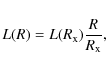
We denote the angle between the radial direction and the slow-mode shock (Fig. A.1) as
![]() .
Taking into account the continuity equation across the SMS
.
Taking into account the continuity equation across the SMS
where
which defines the geometry of the SMSs.
To describe the coronal mass density
![]() ,
we use the isothermal solar-wind model of Parker
(see Mann et al. 1999a) for temperature
,
we use the isothermal solar-wind model of Parker
(see Mann et al. 1999a) for temperature
![]() ,
1.5, and 2 MK, which also provides the corresponding solar-wind speed
,
1.5, and 2 MK, which also provides the corresponding solar-wind speed
![]() .
This, together with the previously defined B(R), also defines the ambient coronal Alfvén velocity
.
This, together with the previously defined B(R), also defines the ambient coronal Alfvén velocity
![]() and plasma-to-magnetic pressure ratio
and plasma-to-magnetic pressure ratio ![]() ,
which both govern the jump relations at the SMS. Assuming that the guiding field is negligible, the density and temperature jump at SMS can be expressed as:
,
which both govern the jump relations at the SMS. Assuming that the guiding field is negligible, the density and temperature jump at SMS can be expressed as:
(Skender et al. 2003; Vrsnak & Skender 2005; Aurass et al. 2002), which determines the density and the temperature of the plasma inflowing into the reconnection outflow jet at a given R.
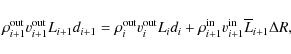
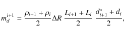
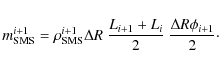
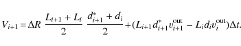
At a given radial distance R, the density of the reconnection outflow is determined by both the
flow carried from lower heights and the flow carried across the SMS. According to the geometry
depicted in Fig. A.1, the continuity equation (mass conservation) can be written in the form:
where
Assuming the spherical geometry, the length L is given by
where
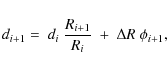
with
Equations (A.1-A.7) estimate the density distribution along the post CME-ray,
![]() ,
for various values of diffusion region height
,
for various values of diffusion region height ![]() .
In Fig. A.2, we show the
results obtained using the coronal magnetic-field model of Dulk & McLean (1978) and Mann et al. (1999b),
whereas for the coronal density, we use the isothermal (106 K) solar-wind model of
Mann et al. (1999a).
.
In Fig. A.2, we show the
results obtained using the coronal magnetic-field model of Dulk & McLean (1978) and Mann et al. (1999b),
whereas for the coronal density, we use the isothermal (106 K) solar-wind model of
Mann et al. (1999a).
![\begin{figure}
\par\includegraphics[width=9cm]{0844fig9.eps}
\end{figure}](/articles/aa/full_html/2009/21/aa10844-08/img119.png) |
Figure A.2: Current sheet number-density calculated using the coronal magnetic field model by Dulk & McLean (1978) and Mann et al. (1999b); thick-black and thick-gray lines, respectively. The solar wind density model by Mann et al. (1999a) is drawn by thin-gray line (denoted as ``corona 106 K''). |
| Open with DEXTER | |
We now consider the plasma temperature along the current sheet. In the first layer above the
X-line, the temperature equals the temperature
![]() evaluated by Eq. (A.4) at the
radial distance
evaluated by Eq. (A.4) at the
radial distance
![]() .
The plasma of this temperature moves
outward and enters into the next layer through the area
.
The plasma of this temperature moves
outward and enters into the next layer through the area
![]() ,
undergoing adiabatic
cooling due to volume expansion. In the second layer, it meets with the plasma that enters into the
current sheet through the slow-mode shock, where it is heated to
,
undergoing adiabatic
cooling due to volume expansion. In the second layer, it meets with the plasma that enters into the
current sheet through the slow-mode shock, where it is heated to
![]() .
The
same happens successively in each additional level.
.
The
same happens successively in each additional level.
Since the thermal conductivity of coronal plasma is very high, the temperature can be assumed to be
uniform across each layer, i.e., along the magnetic field-lines connecting the SMSs (i.e.,
magnetic-field component
![]() ). Thus, we can write for the temperature of a given layer:
). Thus, we can write for the temperature of a given layer:
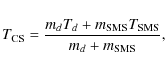
where, md and Td are the mass and temperature, respectively, of the plasma contained in the volume defined by the lines denoted in Fig. A.1 as di and di+1*. We note that we have neglected the thermal conductivity along the CS axis of symmetry, since the heat flow in this direction is reduced due to the magnetic-field component
whereas
where
The estimate of the temperature
![]() in a given layer still requires evaluation of the
temperature Td, where we must take account of the adiabatic expansion from the layer ``i'' to
``i+1''. The plasma contained in the volume defined by lines di-1 and di:
in a given layer still requires evaluation of the
temperature Td, where we must take account of the adiabatic expansion from the layer ``i'' to
``i+1''. The plasma contained in the volume defined by lines di-1 and di:

expands into the volume:
The time

where
where
The system of Eqs. (A.1-A.14) can be solved starting from the first layer above the
diffusion region, and successively calculating the values in every new layer by using the values
obtained for previous layer. In this way, we derive the dependencies ![]() and T(R) for the
current sheet plasma.
and T(R) for the
current sheet plasma.
References
- Asai, A., Yokoyama, T., Shimojo, M., & Shibata, K. 2004, ApJ, 605, L77 [NASA ADS] [CrossRef] (In the text)
- Aschwanden, M. J., Kosugi, T., Hudson, H. S., Wills, M. J., & Schwartz, R. A. 1996, ApJ, 470, 1198 [NASA ADS] [CrossRef] (In the text)
- Aurass, H., Vrsnak, B., & Mann, G. 2002, A&A, 384, 273 [NASA ADS] [CrossRef] [EDP Sciences] (In the text)
- Bárta, M., Vrsnak, B., & Karlický, M. 2008, A&A, 477, 649 [NASA ADS] [CrossRef] [EDP Sciences] (In the text)
- Bemporad, A., Poletto, G., Suess, S. T., et al. 2006, ApJ, 638, 1110 [NASA ADS] [CrossRef]
- Bemporad, A., Poletto, G., Landini, F., & Romoli, M. 2008, Ann. Geophys., in press (In the text)
- Billings, D. E. 1966, A guide to the solar corona (New York: Academic Press) (In the text)
- Brueckner, G. E., Howard, R. A., Koomen, M. J., et al. 1995, Sol. Phys., 162, 357 [NASA ADS] [CrossRef] (In the text)
- Carmichael, H. 1964, in The Physics of Solar Flares, ed. W. N. Hess, 451 (In the text)
- Ciaravella, A., & Raymond, J. C. 2008, ApJ, in press
- Ciaravella, A., Raymond, J. C., Li, J., et al. 2002, ApJ, 575, 1116 [NASA ADS] [CrossRef]
- Dulk, G. A., & McLean, D. J. 1978, Sol. Phys., 57, 279 [NASA ADS] [CrossRef] (In the text)
- Forbes, T. G., & Acton, L. W. 1996, ApJ, 459, 330 [NASA ADS] [CrossRef] (In the text)
- Forbes, T. G., Linker, J. A., Chen, J., et al. 2006, Space Sci. Rev., 123, 251 [NASA ADS] [CrossRef] (In the text)
- Furth, H. P., Killeen, J., & Rosenbluth, M. N. 1963, Physics of Fluids, 6, 459 [NASA ADS] [CrossRef] (In the text)
- Gary, G. A. 2001, Sol. Phys., 203, 71 [NASA ADS] [CrossRef] (In the text)
- Gekelman, W., & Pfister, H. 1988, Physics of Fluids, 31, 2017 [NASA ADS] [CrossRef] (In the text)
- Hirayama, T. 1974, Sol. Phys., 34, 323 [NASA ADS] [CrossRef] (In the text)
- Innes, D. E., McKenzie, D. E., & Wang, T. 2003a, Sol. Phys., 217, 247 [NASA ADS] [CrossRef] (In the text)
- Innes, D. E., McKenzie, D. E., & Wang, T. 2003b, Sol. Phys., 217, 267 [NASA ADS] [CrossRef]
- Ko, Y.-K., Raymond, J. C., Lin, J., et al. 2003, ApJ, 594, 1068 [NASA ADS] [CrossRef]
- Kohl, J. L., Esser, R., Gardner, L. D., et al. 1995, Sol. Phys., 162, 313 [NASA ADS] [CrossRef] (In the text)
- Kopp, R. A., & Pneuman, G. W. 1976, Sol. Phys., 50, 85 [NASA ADS] [CrossRef] (In the text)
- Lee, J.-Y., Raymond, J. C., Ko, Y.-K., & Kim, K.-S. 2006, ApJ, 651, 566 [NASA ADS] [CrossRef] (In the text)
- Lin, J. 2004, Sol. Phys., 219, 169 [NASA ADS] [CrossRef] (In the text)
- Lin, J., Ko, Y.-K., Sui, L., et al. 2005, ApJ, 622, 1251 [NASA ADS] [CrossRef]
- Mann, G., Jansen, F., MacDowall, R. J., Kaiser, M. L., & Stone, R. G. 1999a, A&A, 348, 614 [NASA ADS] (In the text)
- Mann, G., Klassen, A., Estel, C., & Thompson, B. J. 1999b, in 8th SOHO Workshop: Plasma Dynamics and Diagnostics in the Solar Transition Region and Corona, ed. J.-C. Vial, & B. Kaldeich-Schü, ESA SP, 446, 477 (In the text)
- Maricic, D., Vrsnak, B., Stanger, A. L., et al. 2007, Sol. Phys., 241, 99 [NASA ADS] [CrossRef] (In the text)
- Masuda, S., Kosugi, T., Hara, H., Tsuneta, S., & Ogawara, Y. 1994, Nature, 371, 495 [NASA ADS] [CrossRef] (In the text)
- McKenzie, D. E., & Hudson, H. S. 1999, ApJ, 519, L93 [NASA ADS] [CrossRef] (In the text)
- Parker, E. N. 1958, ApJ, 128, 664 [NASA ADS] [CrossRef] (In the text)
- Petschek, H. E. 1964, in The Physics of Solar Flares, ed. W. N. Hess, 425 (In the text)
- Poland, A. I., Howard, R. A., Koomen, M. J., Michels, D. J., & Sheeley, Jr., N. R. 1981, Sol. Phys., 69, 169 [NASA ADS] [CrossRef] (In the text)
- Poletto, G., Bemporad, A., Landini, F., & Romoli, M. 2008, Ann. Geophys., in press (In the text)
- Raymond, J. C., Ciaravella, A., Dobrzycka, D., et al. 2003, ApJ, 597, 1106 [NASA ADS] [CrossRef] (In the text)
- Riley, P., Linker, J. A., Mikic, Z., et al. 2002, ApJ, 578, 972 [NASA ADS] [CrossRef] (In the text)
- Riley, P., Lionello, R., Mikic, Z., et al. 2007, ApJ, 655, 591 [NASA ADS] [CrossRef] (In the text)
- Roussev, I. I., Forbes, T. G., Gombosi, T. I., et al. 2003, ApJ, 588, L45 [NASA ADS] [CrossRef] (In the text)
- Saez, F., Llebaria, A., Lamy, P., & Vibert, D. 2007, A&A, 473, 265 [NASA ADS] [CrossRef] [EDP Sciences] (In the text)
- Sheeley, Jr., N. R., & Wang, Y.-M. 2002, ApJ, 579, 874 [NASA ADS] [CrossRef] (In the text)
- Sheeley, Jr., N. R., & Wang, Y.-M. 2007, ApJ, 655, 1142 [NASA ADS] [CrossRef] (In the text)
- Sheeley, Jr., N. R., Warren, H. P., & Wang, Y.-M. 2004, ApJ, 616, 1224 [NASA ADS] [CrossRef] (In the text)
- Simnett, G. M., Tappin, S. J., Plunkett, S. P., et al. 1997, Sol. Phys., 175, 685 [NASA ADS] [CrossRef] (In the text)
- Skender, M., Vrsnak, B., & Martinis, M. 2003, Phys. Rev. E, 68, 046405 [NASA ADS] [CrossRef] (In the text)
- Soward, A. M., & Priest, E. R. 1982, J. Plasma Physics, 28, 335 [NASA ADS] [CrossRef]
- Sturrock, P. A. 1966, Nature, 211, 695 [NASA ADS] [CrossRef] (In the text)
- Sui, L., Holman, G. D., & Dennis, B. R. 2004, ApJ, 612, 546 [NASA ADS] [CrossRef] (In the text)
- Sui, L., Holman, G. D., White, S. M., & Zhang, J. 2005, ApJ, 633, 1175 [NASA ADS] [CrossRef]
- Svestka, Z. F., Fontenla, J. M., Machado, M. E., Martin, S. F., & Neidig, D. F. 1987, Sol. Phys., 108, 237 [NASA ADS] [CrossRef] (In the text)
- Török, T., Kliem, B., & Titov, V. S. 2004, A&A, 413, L27 [NASA ADS] [CrossRef] [EDP Sciences] (In the text)
- Tsuneta, S. 1996, ApJ, 456, 840 [NASA ADS] [CrossRef] (In the text)
- Tsuneta, S., Hara, H., Shimizu, T., et al. 1992, PASJ, 44, L63 [NASA ADS] (In the text)
- Ugai, M. 1987, Geophys. Res. Lett., 14, 103 [NASA ADS] [CrossRef] (In the text)
- Veronig, A. M., Karlický, M., Vrsnak, B., et al. 2006, A&A, 446, 675 [NASA ADS] [CrossRef] [EDP Sciences] (In the text)
- Vourlidas, A., Buzasi, D., Howard, R. A., & Esfandiari, E. 2002, in Solar Variability: From Core to Outer Frontiers, ed. J. Kuijpers, ESA SP, 506, 91 (In the text)
- Vourlidas, A., Subramanian, P., Dere, K. P., & Howard, R. A. 2000, ApJ, 534, 456 [NASA ADS] [CrossRef] (In the text)
- Vrsnak, B. 2008, Annales Geophysicae, 26, 3089 [NASA ADS] (In the text)
- Vrsnak, B., & Skender, M. 2005, Sol. Phys., 226, 97 [NASA ADS] [CrossRef]
- Vrsnak, B., Magdalenic, J., Aurass, H., & Mann, G. 2002, A&A, 396, 673 [NASA ADS] [CrossRef] [EDP Sciences] (In the text)
- Vrsnak, B., Klein, K.-L., Warmuth, A., Otruba, W., & Skender, M. 2003, Sol. Phys., 214, 325 [NASA ADS] [CrossRef] (In the text)
- Vrsnak, B., Magdalenic, J., & Zlobec, P. 2004, A&A, 413, 753 [NASA ADS] [CrossRef] [EDP Sciences] (In the text)
- Vrsnak, B., Temmer, M., Veronig, A., Karlický, M., & Lin, J. 2006, Sol. Phys., 234, 273 [NASA ADS] [CrossRef] (In the text)
- Wang, Y.-M., Sheeley, N. R., Howard, R. A., St. Cyr, O. C., & Simnett, G. M. 1999, Geophys. Res. Lett., 26, 1203 [NASA ADS] [CrossRef] (In the text)
- Webb, D. F., & Cliver, E. W. 1995, J. Geophys. Res., 100, 5853 [NASA ADS] [CrossRef] (In the text)
- Webb, D. F., Burkepile, J., Forbes, T. G., & Riley, P. 2003, J. Geophys. Res. (Space Physics), 108, 1440 [NASA ADS] [CrossRef]
- Yokoyama, T., Akita, K., Morimoto, T., Inoue, K., & Newmark, J. 2001, ApJ, 546, L69 [NASA ADS] [CrossRef]
All Tables
Table 1: Spectrographic results on the UV current sheets.
All Figures
| |
Figure 1:
a) Interpretation of the ray in terms of the Petschek (1964) reconnection model: DR - diffusion region; SMS - slow mode shocks (dashed lines intersecting at DR); PEL - post-eruption loops. Magnetic field-lines are drawn by thin lines; gray area between the SMSs outlines the post-CME ray. The coordinate system is indicated (the line of sight is in y-direction). b) An element of bifurcated current sheet; arrows mark plasma flows (
|
| Open with DEXTER | |
| In the text | |
| |
Figure 2:
Dependence of the width and morphology of the ray at a given height on the orientation/geometry of the current sheet: a) straight CS; b) wavy CS. The CS half-thickness is denoted by d, horizontal length (i.e., the length in xy-plane, see also Fig. 1) by L, the ray width by D, and the inclination to the line of sight (LoS) by |
| Open with DEXTER | |
| In the text | |
| |
Figure 3:
a) Simple post-CME ray (9 January 2002 at 06:06 UT); b) complex ray consisting of three radial substructures (9 January 2002 at 02:30 UT). The ray is marked by white arrow. The scale of the LASCO-C2 images is given in pixels (1 pixel corresponds to 11.9 arcsec). The column-mass profiles measured along the bin marked by white lines are shown in the right-hand panels (abscissa scale in pixels). Estimates of the ray width, D, and column-mass excess, |
| Open with DEXTER | |
| In the text | |
| |
Figure 4: The five measured post-CME rays (indicated by arrows in the full-resolution LASCO-C2 images shown in the first column): a- c) 9 January 2002 at 00:06, 06:06, and 12:06 UT, respectively; d) 18 November 2003 at 12:50 UT; e) 26 June 2005 at 06:30 UT. In the second, third, and fourth column we show the ray width, column-mass excess, and the density excess, as a function of the radial distance. The widths and radial distances are expressed in units of the solar radius. The least-square fits are shown in the insets, together with the correlation coefficient C. |
| Open with DEXTER | |
| In the text | |
| |
Figure 5:
Number of electrons per unit length of the ray,
|
| Open with DEXTER | |
| In the text | |
| |
Figure 6:
a) LASCO-C2 running-difference images of the west-limb ray of 8 January 2002 (13:54 UT), revealing the inflow into the ray. The slice used in the stack-plot shown in b) is outlined by white rectangle centered at
|
| Open with DEXTER | |
| In the text | |
| |
Figure 7:
a) Comparison of the density-excess measurements presented in the right hand column of Fig. 4 with the model results (thin black lines labeled by the heliocentric distance of the diffusion region, |
| Open with DEXTER | |
| In the text | |
| |
Figure A.1: Geometry of the post-CME ray model. Dash-dotted lines depict the axis of symmetry, shaded area represents the slow mode shock (SMS) and dotted lines the local radial direction. Local coordinate system is indicated in the lower-right corner. For details see the text in the Appendix. |
| Open with DEXTER | |
| In the text | |
| |
Figure A.2: Current sheet number-density calculated using the coronal magnetic field model by Dulk & McLean (1978) and Mann et al. (1999b); thick-black and thick-gray lines, respectively. The solar wind density model by Mann et al. (1999a) is drawn by thin-gray line (denoted as ``corona 106 K''). |
| Open with DEXTER | |
| In the text | |
Copyright ESO 2009
Current usage metrics show cumulative count of Article Views (full-text article views including HTML views, PDF and ePub downloads, according to the available data) and Abstracts Views on Vision4Press platform.
Data correspond to usage on the plateform after 2015. The current usage metrics is available 48-96 hours after online publication and is updated daily on week days.
Initial download of the metrics may take a while.