| Issue |
A&A
Volume 499, Number 2, May IV 2009
|
|
|---|---|---|
| Page(s) | 357 - 369 | |
| Section | Cosmology (including clusters of galaxies) | |
| DOI | https://doi.org/10.1051/0004-6361/200810838 | |
| Published online | 24 February 2009 | |
The REFLEX galaxy cluster survey
VIII. Spectroscopic observations
and optical atlas![[*]](/icons/foot_motif.png) ,
,
L. Guzzo1,2 - P. Schuecker2 - H. Böhringer2 - C. A. Collins3 - A. Ortiz-Gil1,4 - S. De Grandi1 - A. C. Edge5 - D. M. Neumann6 - S. Schindler7 - C. Altucci1 - P. A. Shaver8
1 - INAF - Osservatorio Astronomico di Brera, via Bianchi 46, 23807
Merate (LC), Italy
2 - Max-Planck-Institut für extraterrestrische Physik,
Giessenbachstraße 1, 85740 Garching, Germany
3 - Astrophysics Research Institute, Liverpool John Moores University, Twelve Quays House, Egerton Wharf, Birkenhead CH41 1LD, UK
4 - Observatori Astronomic - Universitat de Valencia,
Edificio de Institutos de Investigacion, Aptdo. Correos 22085,
46071 Valencia, Spain
5 - Physics Department, University of Durham, South Road, Durham DH1 3LE, UK
6 - CEA Saclay, Service d'Astrophysique, Gif-sur-Yvette, France
7 - Institute for Astro- and Particle Physics, Universität Innsbruck, 6020 Innsbruck, Austria
8 - European Southern Observatory, 85748 Garching, Germany
Received 21 August 2008 / Accepted 16 December 2008
Abstract
We present the final data from the spectroscopic survey of the
ROSAT-ESO Flux-Limited X-ray (REFLEX) catalog of galaxy clusters. The REFLEX survey covers 4.24 steradians (34% of the entire sky) below a declination of
![]() and at
high Galactic latitude (
and at
high Galactic latitude (
![]() ). The REFLEX catalog
includes 447 entries with a median redshift of 0.08 and is better than
). The REFLEX catalog
includes 447 entries with a median redshift of 0.08 and is better than ![]() complete to a
limiting flux
complete to a
limiting flux
![]() (0.1 to 2.4 keV), representing the largest statistically
homogeneous sample of clusters drawn from the ROSAT All-Sky Survey
(RASS) to date. Here we describe the details
of the spectroscopic observations carried out at the ESO 1.5 m, 2.2 m,
and 3.6 m telescopes, as well as the data reduction and redshift measurement techniques. The spectra typically cover the wavelength range 3600-7500 Å at a two-pixel resolution of
(0.1 to 2.4 keV), representing the largest statistically
homogeneous sample of clusters drawn from the ROSAT All-Sky Survey
(RASS) to date. Here we describe the details
of the spectroscopic observations carried out at the ESO 1.5 m, 2.2 m,
and 3.6 m telescopes, as well as the data reduction and redshift measurement techniques. The spectra typically cover the wavelength range 3600-7500 Å at a two-pixel resolution of ![]() 14 Å, and the measured redshifts have a total rms error of
14 Å, and the measured redshifts have a total rms error of ![]() 100 km s-1. In total we present 1406 new galaxy redshifts in 192 clusters, most of which previously did not have any redshift measured. Finally, the luminosity/redshift
distributions of the cluster sample and a comparison to the no-evolution
expectations from the cluster X-ray luminosity function are
presented.
100 km s-1. In total we present 1406 new galaxy redshifts in 192 clusters, most of which previously did not have any redshift measured. Finally, the luminosity/redshift
distributions of the cluster sample and a comparison to the no-evolution
expectations from the cluster X-ray luminosity function are
presented.
Key words: surveys - galaxies: clusters: general - galaxies: distances and redshifts
1 Introduction
Clusters of galaxies represent the largest collapsed objects in the
hierarchy of cosmic structures, stemming from the growth of
fluctuations lying on the high-density tail of the matter density
field (Kaiser 1986). As such, their number density and evolution are
strongly dependent on the normalization of the power spectrum and the
value of the density parameter
![]() (e.g. Borgani & Guzzo 2001;
Rosati et al. 2002). In addition, the physics involved in
``illuminating'' clusters and making them visible is in principle
easier to understand than the various complex processes
connected to the formation and evolution of stars in galaxies (although a
drawback can be that their typical dynamical time is long, comparable
to the Hubble time). In particular in the X-ray band, where clusters
can be defined and recognised as single objects (not just as a mere
collection of galaxies), observable quantities like X-ray luminosity
(e.g. Borgani & Guzzo 2001;
Rosati et al. 2002). In addition, the physics involved in
``illuminating'' clusters and making them visible is in principle
easier to understand than the various complex processes
connected to the formation and evolution of stars in galaxies (although a
drawback can be that their typical dynamical time is long, comparable
to the Hubble time). In particular in the X-ray band, where clusters
can be defined and recognised as single objects (not just as a mere
collection of galaxies), observable quantities like X-ray luminosity
![]() and temperature
and temperature ![]() show scaling relations with the total
mass (and thus to the mass of the dark-matter halo, e.g. Evrard et al. 1996; Allen et al. 2001; Reiprich & Böhringer 2002; Ettori et al. 2004). A full comprehension of these scaling relations requires
more ingredients than the simple conversion of gravitational potential
energy into heat during the growth of fluctuations (Kaiser 1986;
Helsdon & Ponman 2000; Finoguenov et al. 2001; Borgani et al. 2004).
Nevertheless, these relations allow us to use clusters to test the
mass function and the mass power spectrum, respectively via the
observed cluster X-ray luminosity function (XLF) and clustering,
(e.g. Böhringer et al. 2002; Pierpaoli et al. 2003;
Schuecker et al. 2003a).
show scaling relations with the total
mass (and thus to the mass of the dark-matter halo, e.g. Evrard et al. 1996; Allen et al. 2001; Reiprich & Böhringer 2002; Ettori et al. 2004). A full comprehension of these scaling relations requires
more ingredients than the simple conversion of gravitational potential
energy into heat during the growth of fluctuations (Kaiser 1986;
Helsdon & Ponman 2000; Finoguenov et al. 2001; Borgani et al. 2004).
Nevertheless, these relations allow us to use clusters to test the
mass function and the mass power spectrum, respectively via the
observed cluster X-ray luminosity function (XLF) and clustering,
(e.g. Böhringer et al. 2002; Pierpaoli et al. 2003;
Schuecker et al. 2003a).
In addition to providing a fairly direct connection of observed quantities to model (mass-specific) predictions, X-ray based cluster surveys have further crucial advantages over optically-selected catalogs: first, X-ray emission is proportional to the gas density squared, and thus is more concentrated and less sensitive to projection effects than the simple galaxy density profile. Secondly, the selection function of an X-ray cluster survey is essentially that of a flux-limited sample, and thus fairly easy to reconstruct. This is a crucial feature when the goal is to use these samples for cosmological measurements that necessarily involve a precise knowledge of the sampled volume, as it is the case when computing first or second moments of the density field.
The advent of the ROSAT All-Sky Survey (RASS, Voges et al. 1999) at
the beginning of the 1990's, opened up for the first time the
possibility to construct X-ray cluster samples over wide areas of the
sky. Optical identification of these clusters was eased by the good
match between the flux limit of the RASS (![]() 10-12 erg s-1 cm-2 for extended sources) and the depth of the only wide-area optical imaging available at the time, i.e. the Palomar and in particular the southern UK-Schmidt sky surveys. These early X-ray samples included surveys like Hydra (Pierre et al. 1994), SGP (Romer et al. 1994; Cruddace et al. 2002, 2003), XBACS (Ebeling et al. 1996), BCS (Ebeling et al. 1998, 2000), RASS-BS (De Grandi et al. 1999),
NORAS (Böhringer et al. 2000), NEP (Henry et al. 2001; Gioia et al. 2003). Some of these early
studies concentrated on X-ray detections of optically-selected
clusters, i.e. typically systems previously identified optically by
Abell (1958) and Abell et al. (1989), as notably the XBACS catalog or the surveys of Burns and collaborators (Burns et al. 1996; Ledlow et al. 1999). However, some others, as the SGP, BCS and RASS-BS surveys, were initial steps towards the goal of constructing a
complete, X-ray selected statistical sample covering the whole sky, or
at least the Southern hemisphere where deeper panoramic imaging was
provided by the digitization of the ESO-SRC III-aJ (
10-12 erg s-1 cm-2 for extended sources) and the depth of the only wide-area optical imaging available at the time, i.e. the Palomar and in particular the southern UK-Schmidt sky surveys. These early X-ray samples included surveys like Hydra (Pierre et al. 1994), SGP (Romer et al. 1994; Cruddace et al. 2002, 2003), XBACS (Ebeling et al. 1996), BCS (Ebeling et al. 1998, 2000), RASS-BS (De Grandi et al. 1999),
NORAS (Böhringer et al. 2000), NEP (Henry et al. 2001; Gioia et al. 2003). Some of these early
studies concentrated on X-ray detections of optically-selected
clusters, i.e. typically systems previously identified optically by
Abell (1958) and Abell et al. (1989), as notably the XBACS catalog or the surveys of Burns and collaborators (Burns et al. 1996; Ledlow et al. 1999). However, some others, as the SGP, BCS and RASS-BS surveys, were initial steps towards the goal of constructing a
complete, X-ray selected statistical sample covering the whole sky, or
at least the Southern hemisphere where deeper panoramic imaging was
provided by the digitization of the ESO-SRC III-aJ (![]() )
plates (through e.g. the Edinburgh-based COSMOS catalog, McGillivray & Stobie 1984, or the APM survey, Maddox et al. 1990).
)
plates (through e.g. the Edinburgh-based COSMOS catalog, McGillivray & Stobie 1984, or the APM survey, Maddox et al. 1990).
Table 1: Complete log of the spectroscopic observations.
![\begin{figure}
\par\includegraphics[width=14cm,clip]{0838f1.ps}
\end{figure}](/articles/aa/full_html/2009/20/aa10838-08/img27.png) |
Figure 1:
The distribution on the sky of the 447 clusters composing the
REFLEX sample with
|
| Open with DEXTER | |
This goal has been achieved with the completion of the REFLEX
(ROSAT-ESO Flux Limited X-ray) cluster survey, whose optical
identification and spectroscopic survey are described here. REFLEX
combines the X-ray data from the RASS and ESO follow-up optical
observations to construct a complete flux-limited sample of 447 clusters with flux limit
![]() erg s-1 cm-2 (in the ROSAT energy band, 0.1-2.4 keV). It covers the Southern sky up to
erg s-1 cm-2 (in the ROSAT energy band, 0.1-2.4 keV). It covers the Southern sky up to
![]() ,
excluding the band of the Milky Way (
,
excluding the band of the Milky Way (
![]() )
to avoid high NH column densities and crowding by stars. For the same reason, the regions of the Magellanic clouds are also excised from the survey (see Table 1 in Böhringer et al. 2001a, Paper I hereafter), totaling an overall area of 13 924
)
to avoid high NH column densities and crowding by stars. For the same reason, the regions of the Magellanic clouds are also excised from the survey (see Table 1 in Böhringer et al. 2001a, Paper I hereafter), totaling an overall area of 13 924 ![]() or 4.24 sr. The overall sky distribution of REFLEX clusters is shown in Fig. 1.
or 4.24 sr. The overall sky distribution of REFLEX clusters is shown in Fig. 1.
REFLEX provides the largest statistically complete
X-ray-selected cluster sample to date. The volume of Universe it
probes is bigger than that covered by any present galaxy redshift
survey except for the Sloan Digital Sky Survey, which goes to
slightly larger depth but covers about half the sky area of REFLEX. We note that the RASS still remains today the only all-sky X-ray survey performed with an
imaging X-ray telescope. We also note that the potential of
the RASS for cluster research has not been fully exploited yet. There
are two ongoing efforts in this direction. The REFLEX-2 survey is
extending REFLEX to a fainter flux limit of
![]() erg s-1 cm-2. This sample
will contain more than 400 new clusters, part of which have been
already observed spectroscopically during the ESO Key Programme described in this
paper. Complementarily, the MACS survey (Ebeling et al. 2001, 2007)
aims specifically at identifying all luminous X-ray clusters at z>0.3 still hiding in the RASS, probing an even bigger volume of the Universe.
erg s-1 cm-2. This sample
will contain more than 400 new clusters, part of which have been
already observed spectroscopically during the ESO Key Programme described in this
paper. Complementarily, the MACS survey (Ebeling et al. 2001, 2007)
aims specifically at identifying all luminous X-ray clusters at z>0.3 still hiding in the RASS, probing an even bigger volume of the Universe.
The overall goal of REFLEX has been to map a large volume of the Universe using clusters, such that the survey could be used both to measure large-scale structure and as a controlled source for studying the physical properties of clusters. These requirements imposed a high standard to the whole X-ray source selection and identification process, which is described in detail in Böhringer et al. (2004, Paper II hereafter). In this paper, we present the data from the spectroscopic survey conducted with ESO telescopes to identify and measure the redshifts of REFLEX clusters. In particular, we report all relevant information on individual galaxy redshift data. We also provide (in electronic form), finding charts and optical/X-ray overlays of the clusters. These allow a first qualitative inspection of their main morphological properties (as e.g. their concentration or the presence of a dominant cD galaxy), which we hope will stimulate further quantitative work on this sample.
The complete REFLEX survey has been used over the last few years to measure fundamental cosmological quantities in the ``local'' Universe. These include, among others:

- the cluster X-ray luminosity function (Böhringer et al. 2002), and from this the mean abundance of clusters;
-
- the two-point correlation function of the cluster
distribution (Collins et al. 2000);
-
- the power spectrum of the cluster distribution (Schuecker et al. 2001, 2002);
-
- the values of the cosmic mean density of matter
 and the power spectrum normalization
  ,
via the combination of the above observables (Schuecker et al. 2003a);
,
via the combination of the above observables (Schuecker et al. 2003a);
-
- the Gaussianity of the cluster distribution, as described by Minkowski functionals (Kersher et al. 2001);
-
- the value of the equation of state parameter of dark energy w (Schuecker et al. 2003b);
-
- the relation between cluster velocity dispersions (measurable for a sub-sample of 170 clusters) and X-ray luminosity (Ortiz-Gil et al. 2004);
-
- the cluster-galaxy correlation function (Sanchez et al. 2005);
-
- the influence of scaling relation uncertainties on the estimate of cosmological parameters (Stanek et al. 2006).
The paper is organized as follows: in Sect. 2 we provide a quick overview
of the selection and identification strategy of the REFLEX survey; in Sect. 3 we present the spectroscopic observations and discuss the observations, data reduction and redshift measurement technique; in Sect. 4 we present the spectroscopic catalog and the related finding
charts and optical overlays; in Sect. 5 we discuss some properties of the redshift and luminosity distributions of REFLEX cluster; finally, in Sect. 6 we conclude and summarize the content of the paper. We adopt a ``concordance'' cosmological model, with
![]() km s-1 Mpc-1,
km s-1 Mpc-1,
![]() ,
,
![]() ,
and - unless specified - quote all X-ray
fluxes and luminosities in the ROSAT [0.1-2.4] keV band.
,
and - unless specified - quote all X-ray
fluxes and luminosities in the ROSAT [0.1-2.4] keV band.
2 REFLEX identification strategy: overview
We summarize here, for completeness, the main stages that led to the construction of the cluster candidate sample for REFLEX. A more comprehensive description can be found in Papers I and II.
The X-ray data for all sources detected in the RASS at declinations
smaller than ![]() were analysed using the ``Growth Curve
Analysis'' (GCA) method (Böhringer et al. 2000), thus re-measuring
their flux and geometrical properties. The results are used to produce a flux-limited sample of RASS sources with
were analysed using the ``Growth Curve
Analysis'' (GCA) method (Böhringer et al. 2000), thus re-measuring
their flux and geometrical properties. The results are used to produce a flux-limited sample of RASS sources with
![]() erg s-1 cm-2. This redetermination of the fluxes has been shown to be crucial for extended RASS sources, as are the
majority of REFLEX clusters (Ebeling et al. 1996; De Grandi et al. 1997; Böhringer et al. 2000). Cluster candidates were then found correlating all sources with galaxy density enhancements in the
COSMOS optical data base, obtained from digital scans of the UK Schmidt survey plates at the Royal Observatory Edinburgh (MacGillivray & Stobie 1984; Heydon-Dumbleton et al. 1989), with a density
threshold low enough as to guarantee our desired final completeness of
better than 90%. This meant accepting a contamination of
erg s-1 cm-2. This redetermination of the fluxes has been shown to be crucial for extended RASS sources, as are the
majority of REFLEX clusters (Ebeling et al. 1996; De Grandi et al. 1997; Böhringer et al. 2000). Cluster candidates were then found correlating all sources with galaxy density enhancements in the
COSMOS optical data base, obtained from digital scans of the UK Schmidt survey plates at the Royal Observatory Edinburgh (MacGillivray & Stobie 1984; Heydon-Dumbleton et al. 1989), with a density
threshold low enough as to guarantee our desired final completeness of
better than 90%. This meant accepting a contamination of ![]()
![]() by non-cluster sources spuriously associated with fluctuations in the
galaxy background counts.
The procedure ensures that the selection effects introduced by the
optical identification process are minimized and negligible for our
purpose (see also the statistics given in Paper I). Further tests
provide support that a figure comfortably larger than 90% also
describes the overall detection completeness of the flux-limited
cluster sample in the survey area.
by non-cluster sources spuriously associated with fluctuations in the
galaxy background counts.
The procedure ensures that the selection effects introduced by the
optical identification process are minimized and negligible for our
purpose (see also the statistics given in Paper I). Further tests
provide support that a figure comfortably larger than 90% also
describes the overall detection completeness of the flux-limited
cluster sample in the survey area.
The resulting candidate list was then carefully checked against the available X-ray/optical information and with literature data, to eliminate obvious contaminants prior to the deeper optical follow-up observation program at La Silla. The adopted scheme was very conservative, again accepting a larger contamination (to be cleaned afterwards by the follow-up observations) to guarantee the highest possible completeness in the final sample (see Paper I for details).
The follow-up optical observations of REFLEX clusters were started at
ESO in May 1992. With an ``ESO Key Programme'' status, the survey obtained an overall allocation of 90 nights, distributed among the ESO 3.6 m, 2.2 m and 1.5 m telescopes. A few additional nights were further obtained at the end of the project to partly compensate for the time lost due to bad weather. The complete observing ![]() of the survey is presented in Table 1.
of the survey is presented in Table 1.
The goal of these observations was twofold: a) obtain a definitive identification of ambiguous candidates; b) obtain a measurement of the mean cluster redshift. First, a number of candidate clusters required direct CCD imaging and/or spectroscopy to be safely included in the sample. For example, candidates characterised by a poor appearance on the Sky Survey IIIa-J plates, with no dominant central galaxy or featuring a seemingly point-like X-ray emission had to pass further investigation. In this case, either the object at the X-ray peak was studied spectroscopically, or a short CCD image plus a spectrum of the 2-3 objects nearest to the X-ray peak were taken. This operation was preferentially scheduled at the two smaller telescopes (1.5 m and 2.2 m, see below). In this way, a few AGN's were discovered. When the overall information available (e.g. X-ray hardness ratio, source shape) was consistent with the AGN dominating the emission, the corresponding candidate was rejected from the main list. This is described in full detail in Paper II, where also a list of the more uncertain or ambiguous cases in the REFLEX catalog is presented and discussed thoroughly.
For the bonafide clusters, the final goal of the optical observations
was then to secure a reliable redshift. The observing strategy was
designed as a compromise between the desire of having several
redshifts per cluster, coping with the multiplexing limits of the
available instrumentation, and the large number of clusters to be
measured. Previous experience on the similar Edinburgh/Milano Survey
of EDCC clusters (Collins et al. 1995), had shown the importance of
not relying on just one or two galaxies to measure the cluster
redshift, especially for clusters without a dominant cD galaxy. However, the additional information provided by the detection and localisation of X-rays makes the issues of projection -
that make multiple member redshifts vital for optical samples - much
less severe here![]() .
.
EFOSC1 in MOS mode was a perfect instrument for getting quick redshift measurements for 10-15 galaxies at once, but only for systems that could reasonably fit within the small field of view of the instrument (5.2 arcmin side in imaging with the Tektronics CCD #26, but less than 3 arcmin for spectroscopy in MOS mode, due to hardware/software limitations in the making of the MOS masks). This feature made this combination useful only for clusters above
![]() ,
i.e. where at least the core region could be accommodated within the available area (a core radius of
,
i.e. where at least the core region could be accommodated within the available area (a core radius of
![]() is seen under an angle of 1.3 arcmin at such redshift, in the adopted cosmology).
is seen under an angle of 1.3 arcmin at such redshift, in the adopted cosmology).
The other important aspect of this instrumental set-up is that in several cases, after removal of background/foreground objects one is still left with 8-10 galaxy redshifts within the cluster, by which a first estimate of the cluster velocity dispersion can be attempted. This has been done, complementing the data described here with literature redshifts, for a sub-sample of 170 REFLEX clusters, allowing us to study the scaling relation between cluster velocity dispersion and X-ray luminosity (Ortiz-Gil et al. 2004).
At lower redshifts, doing efficient multi-object spectroscopy work on cluster fields would have required a MOS spectrograph with a larger field of view, i.e. 20-30 arcmin diameter. One possible choice could have been the formerly available ESO fibre spectrograph Optopus (Avila et al. 1989), but its efficiency in terms of numbers of targets observable per night was too low for covering the several hundred clusters we had in our sample. We found the best solution was to split the work between the 1.5 m and 2.2 m telescopes. Clearly, this required accepting some compromise in our initial goal of having multiple redshifts for each cluster. As discussed in Paper II, about half of the cluster redshifts are measured with 5 or more member galaxies, but 42 of them featuring only one galaxy redshift. Most of these cases come from the literature, and the available telescope budget did not allow for a re-determination of these values. For most of these cases, however, the reliability of these single redshift as estimators of the mean systemic redshift is high, as they refer to the brightest cluster galaxy at the centre of X-ray emission. Indeed, as mentioned above, the coupling of the galaxy positions with the X-ray contours is of strong help in indicating which galaxies have the highest probability to be cluster members.
During 8 years of work, we have observed spectroscopically a total of
about 500 cluster candidates, collecting over 3200 galaxy spectra. In this paper, we present the spectroscopic data belonging to the current, published REFLEX sample with
![]() erg s-1 cm-2, which include
erg s-1 cm-2, which include ![]() 1500 spectra. The remaining spectra belong to clusters extending to fainter fluxes, which will form part of a deeper REFLEX-2 sample reaching to
1500 spectra. The remaining spectra belong to clusters extending to fainter fluxes, which will form part of a deeper REFLEX-2 sample reaching to
![]() erg s-1 cm-2.
erg s-1 cm-2.
3 Spectroscopy
3.1 Observations
As detailed in Table 1, all spectroscopic observations were performed at the ESO La Silla observatory, using the 3.6 m, 2.2 m and 1.5 m telescopes. In the following, we describe the instrumental set-ups and main data properties for each of them.
3.1.1 EFOSC1/2@3.6 m observations
About 80% (in terms of number of spectra) of all the REFLEX survey observations were carried out using the 3.6 m telescope with the ESO Faint Object Spectrograph and Camera (EFOSC) in its two incarnations - EFOSC1 and EFOSC2. The EFOSC instruments are high-efficiency transmission spectrographs, with multi-object spectroscopic capability (MOS) and fast switching to imaging mode. This latter feature allows very accurate slit positioning on faint objects. At the time of completing this paper (2008), EFOSC-2 is still actively used at the 3.6 m telescope.
Table 1 shows how during the development of the survey
different detectors were installed on the EFOSCs, following the
evolution of CCD's technology. The EFOSCs were mostly used in MOS mode, which entailed producing
aluminium masks of the cluster fields, on which slitlets of 5-30 arcsec length were carved following a direct image taken with the same instrument. The
masks were then inserted into free positions in the aperture wheel of
the spectrograph. The width of the slits was always of 2-arcsec, the
same width used for single-slit observations. Depending on the
available CCD-grism combination, which varied during the survey, we
worked at dispersions ranging between 130 and
![]() ,
usually aiming at a wavelength coverage between
,
usually aiming at a wavelength coverage between
![]() and
and
![]() .
Most of the 3.6 m observations were performed using
EFOSC-1 with the B300 grism at
.
Most of the 3.6 m observations were performed using
EFOSC-1 with the B300 grism at
![]() and a Tektronics
and a Tektronics
![]() chip, yielding a resolution of
chip, yielding a resolution of
![]() per pixel. This corresponds to a spectral resolution (as measured on a purely instrumentally broadened line) of
per pixel. This corresponds to a spectral resolution (as measured on a purely instrumentally broadened line) of ![]() 2 pixels FWHM, providing radial velocity errors well below 100
2 pixels FWHM, providing radial velocity errors well below 100
![]() for good S/N ratio spectra obtained from
two consecutive exposures of 10-15 mn each (see Sect. 3.3.3
for details). On average each mask contained 15-20 slitlets, over
the available
for good S/N ratio spectra obtained from
two consecutive exposures of 10-15 mn each (see Sect. 3.3.3
for details). On average each mask contained 15-20 slitlets, over
the available
![]() arcmin2 field of view. Standard
calibration observations were collected, as discussed in more detail in Sect. 3.2.
A number of single-slit observations were also carried out at the 3.6 m
telescope, with a similar set-up, especially near the end of the
survey, targeting some of the most distant clusters in the sample.
arcmin2 field of view. Standard
calibration observations were collected, as discussed in more detail in Sect. 3.2.
A number of single-slit observations were also carried out at the 3.6 m
telescope, with a similar set-up, especially near the end of the
survey, targeting some of the most distant clusters in the sample.
3.1.2 EFOSC2@2.2 m and B&C@1.5 m observations
A fraction of the spectroscopic observations were carried out in
single-slit mode using either EFOSC-2 at the
![]() telescope,
(before this instrument was moved to the 3.6 m telescope in January
1998), or the 1.5 m telescope, equipped with a classical Boller & Chivens spectrograph coupled with an RCA (1992) or Ford (1993 onwards) CCD. The latter had very poor response in the blue range, i.e. below 4500 Å, where some of the most interesting absorption lines (e.g. Calcium H and K, G-band) fall for galaxies at low redshift. Thus, the 1.5 m telescope was essentially reserved to observe the brightest members (up to
telescope,
(before this instrument was moved to the 3.6 m telescope in January
1998), or the 1.5 m telescope, equipped with a classical Boller & Chivens spectrograph coupled with an RCA (1992) or Ford (1993 onwards) CCD. The latter had very poor response in the blue range, i.e. below 4500 Å, where some of the most interesting absorption lines (e.g. Calcium H and K, G-band) fall for galaxies at low redshift. Thus, the 1.5 m telescope was essentially reserved to observe the brightest members (up to
![]() )
in the more nearby
clusters of the sample, and played a minor role in the overall redshift survey. The spectral setup was similar to that adopted for the EFOSC spectrographs (grating #21, 172 Å mm-1, blaze angle
)
in the more nearby
clusters of the sample, and played a minor role in the overall redshift survey. The spectral setup was similar to that adopted for the EFOSC spectrographs (grating #21, 172 Å mm-1, blaze angle
![]() ).
).
3.2 Data reduction
The data were reduced using the MIDAS (for data prior to 1995) and IRAF spectroscopic packages, using either custom-built programs (for MIDAS) or - for the bulk of the data - the IRAF specific set of procedures (TWODSPEC/APEXTRACT). The set of operations performed on the available long-slit or MOS spectroscopic CCD frames followed the usual standard procedures, and was essentially the same in both environments. For two observing runs, we repeated the full data reduction using both packages and a direct comparison of the calibrated spectra showed differences well below our typical radial velocity errors (<30 km s-1). In the following, we shall limit ourselves, for simplicity, to the IRAF version of the reduction pipeline which in the end was used for most of the spectra, describing its various phases.
-
- CCD frame inspection, quality check and standardization. These operations included in particular checks for: (a) Possible systematic time dependences of the average bias; (b) possible shifts of the sky lines during the observing run. Sky line positions were also checked after wavelength calibration (see below); (c) similarly, possible shifts of He/Ar/Ne comparison lines at different times during the observing run. All available science and calibration frames were then trimmed to a common size, to eliminate spurious extra borders and overscan regions.
-
- Bias and flat-field corrections. Multiple sets of
bias frames were regularly collected during each observing night and
combined through a 3
 -clipping algorithm (ZEROCOMBINE),
to produce a single, two-dimensional bias frame for that night. In general, the bias frames from the 1.5 m, from the 2.2 m, and from the 3.6 m telescope showed two-dimensional structures at the <0.5 percent level (rms) which are removed by this procedure. To flat-field our spectra only dome flats were typically observed in day time during each run, given that we were not aiming
at precise spectrophotometry. Median flats were constructed for each run using IMCOMBINE.
The number of effectively used flat field exposures for each Single-Slit spectroscopic run ranged between 7 and 40.
In practice, we observed virtually no effect when flat-fielding data
from the 1.5 m and the 3.6 m observations, while this operation was
crucial for most of the data collected at the 2.2 m. Only in the very
last 2.2 m+EFOSC2 run (February 1997) a new CCD (#40) was installed,
eliminating this problem (EFOSC2 was then moved later in that year to
the 3.6 m telescope, where we then performed most of the subsequent
observations). We concluded that there was no gain in flat-fielding the MOS
observations collected at the 3.6 m telescope with EFOSC1 (CCD #26)
and EFOSC2 (CCD #40). Finally the two (or more) science exposures available for every spectroscopic observation were averaged together with IMCOMBINE, after
appropriate scaling and weighting by the the exposure time. This removed very effectively most of the cosmic ray events.
-clipping algorithm (ZEROCOMBINE),
to produce a single, two-dimensional bias frame for that night. In general, the bias frames from the 1.5 m, from the 2.2 m, and from the 3.6 m telescope showed two-dimensional structures at the <0.5 percent level (rms) which are removed by this procedure. To flat-field our spectra only dome flats were typically observed in day time during each run, given that we were not aiming
at precise spectrophotometry. Median flats were constructed for each run using IMCOMBINE.
The number of effectively used flat field exposures for each Single-Slit spectroscopic run ranged between 7 and 40.
In practice, we observed virtually no effect when flat-fielding data
from the 1.5 m and the 3.6 m observations, while this operation was
crucial for most of the data collected at the 2.2 m. Only in the very
last 2.2 m+EFOSC2 run (February 1997) a new CCD (#40) was installed,
eliminating this problem (EFOSC2 was then moved later in that year to
the 3.6 m telescope, where we then performed most of the subsequent
observations). We concluded that there was no gain in flat-fielding the MOS
observations collected at the 3.6 m telescope with EFOSC1 (CCD #26)
and EFOSC2 (CCD #40). Finally the two (or more) science exposures available for every spectroscopic observation were averaged together with IMCOMBINE, after
appropriate scaling and weighting by the the exposure time. This removed very effectively most of the cosmic ray events.
-
- Science and comparison spectra extraction. Two-dimensional spectra corresponding to each slit were then extracted following possible curvature of the spectrum. These
were then reduced to 1-D sky-subtracted spectra using proper sky background regions in the slit. All operations were performed within the APALL/APEXTRACT environment of IRAF.
Corresponding 1D calibration spectra were also extracted at exactly
the same positions from all the available lamp exposures associated
with the target frame. These were typically two He-Ar arc frames,
observed before and after the science exposure. At the 3.6 m
telescope, our direct tests for instrument flexures using 5 strong He
lines at 7 extreme telescope positions showed an rms shift <0.12 pixels, corresponding to 0.744 Å, i.e. 45 km s-1. We concluded that EFOSC flexures over the time of one typical 3.6 m observation (
 30 mn) were negligible, and subsequently used only one calibration lamp. This was not the case at the 1.5 m and 2.2 m telescopes, as shown by
measurements by the ESO staff. For these data, we used both arcs observed before and after the science exposures to compute a time-averaged set of reference lines, as feasible within the IRAF procedures.
30 mn) were negligible, and subsequently used only one calibration lamp. This was not the case at the 1.5 m and 2.2 m telescopes, as shown by
measurements by the ESO staff. For these data, we used both arcs observed before and after the science exposures to compute a time-averaged set of reference lines, as feasible within the IRAF procedures.
![\begin{figure}
\par\includegraphics[width=8.8cm,clip]{0838f2a.eps}\includegraphics[width=8.8cm,clip]{0838f2b.eps}
\end{figure}](/articles/aa/full_html/2009/20/aa10838-08/Timg55.png)
Figure 2: Example of a direct image and spectral lay-out for a cluster observed in MOS mode with EFOSC-1 at the 3.6 m telescope. Left: direct image in white light of RXCJ0658.5-5556, a luminous REFLEX cluster at z=0.2965 (see also Fig. 4). Right: the resulting MOS frame, showing the set of two-dimensional spectra corresponding to each target galaxy in the mask. The dispersion runs along the vertical direction. Each strip shows the sky spectrum (dark horizontal lines) together with the fainter galaxy spectrum.
Open with DEXTER -
- Wavelength calibration. The whole operation was
automatized through the available IRAF procedures (IDENTIFY/REIDENTIFY). In general, an accurate pixel-to-wavelength transformation was determined for the first spectrum of either a full
night of long-slit spectroscopy or a single MOS exposure. The
residuals were directly inspected and discrepant arc line
identifications eliminated. The procedure was iterated until a
satisfactory rms was reached. The relation was then applied to
the science spectrum using DISPCOR.
Typical rms wavelength calibration errors
ranged between 0.3 Å (for the majority of spectra,
e.g. those taken at the 3.6 m telescope), to 1 Å for
lower resolution spectra as those obtained at the 2.2 m telescope with
grism #1. All other spectra in a night-series of long-slit observations were
then calibrated by using the first solution as a guess, using REIDENTIFY. For MOS spectra, however, where large shifts in the
zero point between adjacent spectra are normal (see
Fig. 2), the position of a bright Helium line was used
to provide an approximate zero-point shift for each spectrum. This was
done through a custom-developed script, and provided the first-guess
to calibrate all spectra in a MOS frame with the usual procedure. The
quality and consistency of the final calibration was counter-checked a
posteriori by measuring the position of the three brightest sky lines
([OI]
 5577, NaI 5891, and [OI] 6300),
on the calibrated sky spectrum of each extracted science slit. This
allowed us to spot and correct a few pathological cases.
5577, NaI 5891, and [OI] 6300),
on the calibrated sky spectrum of each extracted science slit. This
allowed us to spot and correct a few pathological cases.
-
- Final cleaning and heliocentric corrections. Before feeding the 1D wavelength-calibrated spectra to the cross-correlation analysis, a number of quality checks and final corrections were performed. These include cleaning of bright sky line residuals (via both an automatic cleaning routine plus visual inspection), computation of heliocentric corrections using the RVCORRECT package (typically smaller than 30 km s-1). Before actually feeding the spectra to the cross-correlation routine, emission lines were removed automatically, as only absorption-line templates were used for the measurement. Emission-line redshifts were estimated separately, using the specific routine EMSAO.
![\begin{figure}
\par\mbox{\includegraphics[width=8.8cm,clip]{0838f3a.ps} \includegraphics[width=8.8cm,clip]{0838f3b.ps} }\end{figure}](/articles/aa/full_html/2009/20/aa10838-08/img57.png) |
Figure 3: Left: differential distribution of the errors on galaxy radial velocities in the REFLEX survey, as estimated by RVSAO. The filled histogram corresponds to considering only cluster member galaxies (i.e. those that were actually used to compute mean cluster redshifts). Collins et al. (1995) showed that total redshift errors amount to typically between 1 and 2 times the internal error estimate by RVSAO, depending inversely on the SNR of the spectrum. Accounting for this, and considering that all spectra around or to the left of the peak of the distribution have very good SNR, we conclude that the typical total error on single galaxy redshifts remains below 100 km s-1. This assures that the dominant source of uncertainty in the mean cluster redshift will be the intrinsic velocity dispersion of the cluster and not a big uncertainty on single galaxy measurements. |
| Open with DEXTER | |
Table 2: Sample page from the full catalog of REFLEX galaxy redshifts (full table available at the CDS and at http://www.brera.inaf.it/REFLEX).
3.3 Redshift measurements
3.3.1 Cross-correlation technique
Galaxy redshifts were estimated from the 1D calibrated spectra, using the classical cross-correlation technique described in detail by Tonry & Davis (1979). This is implemented within the IRAF environment through the package RVSAO (Kurtz & Mink 1998). The basis of the technique is the cross-correlation of the observed galaxy spectrum with a model or template spectrum. This is performed by taking the Fast Fourier Transform of the two spectra, multiplying them together and then transforming back the result to get the Cross-Correlation Function (CCF), whose highest peak is related to the radial velocity difference between the two spectra. Before actually starting this machinery, the two spectra are rebinned into logarithmic bins, so that the relative redshift becomes a linear shift. Then, a number of operations are performed on the spectra, in order to improve the signal-to-noise of the final cross-correlation function. These include continuum subtraction, apodizing and bandpass filtering. All these operations are performed inside the XCSAO routine of RVSAO. We tested several combinations of the command parameters to find the most appropriate set for our spectra. For example, the values for the low- and high-frequency cut-offs of the bandpass filter are specific for the kind of data being used, and optimal values were chosen after experimenting, as to maximize the significance of the CCF. Filtering is important in order to eliminate both the low frequency spurious components left by the subtracted continuum, and the high frequency binning noise. Also, we tested that the redshift estimate was quite insensitive to the exact binwidth (corresponding to 2048 or 4096 bins) chosen in the rebinning. The peak of the CCF was fit by a quadratic polynomial, determining the wavelength shift from its position, and providing an estimate of the uncertainty from its width.
3.3.2 Template spectra
At the core of the cross-correlation technique is the comparison of the object spectrum with a model spectrum of known radial velocity and ideally infinite S/N ratio, the template. The key point of the technique lies in the remarkable similarity in the basic features among galaxy spectra, although the relative intensity of absorption lines can vary quite significantly, in particular when different morphological types are considered. In practice, to cover the range of spectral properties a number of different templates is used for each object and the one producing the highest cross-correlation peak is then taken to be the best model, at the resulting redshift, of the galaxy spectrum being measured.
For measuring the spectra of the REFLEX survey, we benefited of the accurate set of templates constructed by Ettori et al. (1995, EGT hereafter), to which we refer for all details on their properties and construction. This set of templates has a number of useful properties. One advantage is that it includes separate stellar and galaxy spectra together with composite spectra. Another important feature is the accurate knowledge of the template zero points, calibrated in EGT using a set of high-resolution ``primary'' stellar templates.
This template library includes 17 spectra: two high-resolution HD stars with accurately known radial velocity, 3 high S/N galaxies observed with EFOSC in a previous project (Collins et al. 1995), and combined stellar and galaxy spectra built by EGT.
3.3.3 Redshift errors
The major advantage of the cross-correlation technique (Tonry & Davis
1979) is to make use of the complete redshift information contained in
the whole spectrum, not just in the few major identifiable lines.
This pushes the measurement errors well below that expected from the
nominal spectral resolution used. Depending on the SNR of the
spectrum, errors as small as 1/10 of the nominal accuracy on one
single-line measurement are achieved. The specific IRAF
implementation RVSAO computes a confidence level R of the chosen
CCF peak as the ratio of the peak height to the rms background
of the CCF. We empirically verified that estimates with R < 4 have to
be treated with caution, while larger values normally indicated a
rather secure value. We also used the stability of the redshift value
provided by the different templates as an extra figure of merit. Each
galaxy spectrum was cross-correlated against the 17 templates
described above. The overall results for each template were directly
inspected and spectra with 5 or more templates in agreement (within
the redshift errors) and R>4 were passed as secure. Spectra that
did not satisfy these criteria strictly, had in several cases between
2 and 4 templates in agreement. Visual inspection of these cases
often supported the suggested redshift. The typical features of cluster early-type galaxy spectra, as in particular the 4000 Å break, make the visual check of the suggested redshift fairly
straightforward. Spectra were discarded if (1) there was no agreement
between the templates; and (2) the visual inspection did not indicate a
plausible redshift. Once a spectrum had been accepted as secure
(visually or with ![]() 5 templates), the template redshift with the
highest R parameter level was assigned to the galaxy. If several
templates had the same confidence, then the one with the lowest
returned internal error was used. For high signal-to-noise spectra,
it was common to find all the templates agreeing to within a scatter
of
5 templates), the template redshift with the
highest R parameter level was assigned to the galaxy. If several
templates had the same confidence, then the one with the lowest
returned internal error was used. For high signal-to-noise spectra,
it was common to find all the templates agreeing to within a scatter
of
![]() .
The distribution of the
errors for the final redshifts is plotted in Fig. 3.
According to these histograms, the median formal error on our galaxy
redshifts is
.
The distribution of the
errors for the final redshifts is plotted in Fig. 3.
According to these histograms, the median formal error on our galaxy
redshifts is ![]()
![]() ,
with 70% of them being
better than
,
with 70% of them being
better than
![]() .
A small fraction of the
galaxies had emission lines in their spectra. These are indicated in
the redshift catalog, together with the corresponding emission-line
radial velocity. This is normally of lower accuracy than the global,
cross-correlation based redshift which uses the information from the
whole absorption spectrum, and has been used to compute the cluster
redshift only when
no absorption redshift was available. From our previous experience
with the same instrumental set-up (Collins et al. 1995), we also know
that the external error on the radial velocities (measured from repeated observations of the same galaxies) is between a factor of one and two larger than the XCSAO internally estimated value (depending on the SNR). This implies a median value for the total measurement errors
of
.
A small fraction of the
galaxies had emission lines in their spectra. These are indicated in
the redshift catalog, together with the corresponding emission-line
radial velocity. This is normally of lower accuracy than the global,
cross-correlation based redshift which uses the information from the
whole absorption spectrum, and has been used to compute the cluster
redshift only when
no absorption redshift was available. From our previous experience
with the same instrumental set-up (Collins et al. 1995), we also know
that the external error on the radial velocities (measured from repeated observations of the same galaxies) is between a factor of one and two larger than the XCSAO internally estimated value (depending on the SNR). This implies a median value for the total measurement errors
of ![]()
![]() .
.
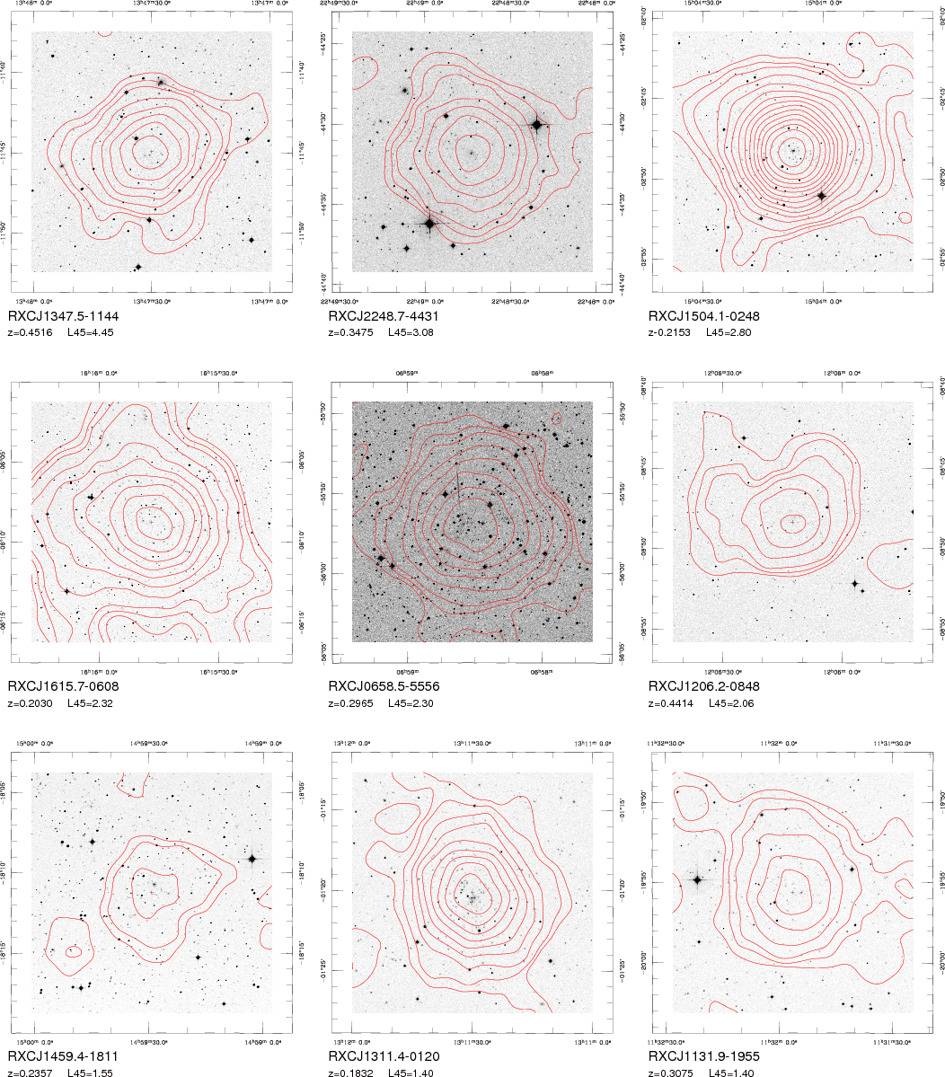 |
Figure 4:
Overlays of the X-ray emission in the [0.5-2.0] KeV band plotted onto the DSS2-RED images of clusters in the REFLEX surveys. The contours correspond to steps of 1 |
| Open with DEXTER | |
![\begin{figure}
\par\includegraphics[width=16cm,clip]{0838f5.eps}
\end{figure}](/articles/aa/full_html/2009/20/aa10838-08/img65.png) |
Figure 5: Composite RGB image of RXCJ1206.2-0848, one of the most spectacular new clusters discovered by the REFLEX survey (the sixth most luminous shown in Fig. 4). This image has been built combining three short (10 mn) direct exposures in the Johnson B, V and R bands taken with EFOSC2 at the ESO 3.6 m telescope and is 5.5 arcmin on a side. Note the dominating cD with very extended yellowish halo, and the prominent blue gravitational lensing candidate arc just westward of it. Several other possible arclets are also visible. |
| Open with DEXTER | |
3.4 Galaxy astrometry
Precise astrometric coordinates were assigned a posteriori to each observed spectrum, since they were available only approximately from the header of the spectroscopic frames. For single-slit observations this was in general straightforward, as (especially at the two smaller telescopes) these involved fairly bright galaxies. For MOS observations, on the other hand, it required a significant amount of work, as unfortunately no electronic information on the astrometric position of target galaxies on the MOS slits is saved along with the observations at the telescope. For this reason, we calibrated astrometrically all the direct CCD images available for each spectroscopic target field, using the USNO2 galaxy catalog and the Starlink's Graphical Astronomy and Image Analysis Tool (GAIA, http://star-www.dur.ac.uk/pdraper/gaia/gaia.html). This was made possible by using the service white-light CCD images used to prepare the EFOSC slit masks, that were appropriately saved at the time of observations. For some fields, images in B and R bands were also available. Inevitably, the final match of the 1D spectra and redshift to their specific galaxy position on the sky was then performed by hand, using the astrometrically calibrated images and the HEDIT IRAF task to write RA and DEC in the spectrum FITS header.
4 Catalog of galaxy redshifts and optical data base
4.1 Galaxy redshift catalog
During our spectroscopic observing campaign, we collected new redshifts for 192 clusters which are included in the current REFLEX catalog. Additionally, a number of systems with X-ray fluxes fainter than the current REFLEX limit were also measured, together with candidates that were subsequently discarded as non-cluster sources. The full list of measured galaxy redshifts for clusters in the REFLEX sample is provided in electronic form only (see www.brera.inaf.it/REFLEX). Here we provide only an excerpt, which is displayed in Table 2. The columns give, respectively: (1) REFLEX name, as defined in Paper II; (2, 3) Coordinates J2000 of each target galaxy; (4) Simple spectral classification, to distinguish among stars, galaxies and clear AGN-like spectra. This classification is not meant to be exhaustive. Additionally, when clear from the available imaging, the spectroscopic measurement of the cD galaxy is explicitly noted; (5) Assignment as a cluster member (+) or interloper (-); (6) heliocentric redshift cz in km s-1, as measured from absorption lines through the cross-correlation procedure; (7) corresponding error; (8) redshift confidence parameter R, giving the ratio between the height of the cross-correlation peak and the overall rms noise of the same function; (9) emission-line redshift, when available; (10, 11) Observation date and telescope; (12) When needed, notes on the spectrum quality or on possible problems in the reduction, astrometry or redshift quality.
4.2 Finding charts and optical/X-ray atlas
A complete optical/X-ray atlas of images for the REFLEX clusters, including finding charts for the spectroscopically measured galaxies is too big to be included in this paper. We have therefore set up a visual atlas of DSS finding charts and X-ray overlays, which is accessible through the survey web page (www.brera.inaf.it/REFLEX). The scientific content of the X-ray overlays and their construction are discussed in a separate paper (Böhringer et al., in preparation). The web page will also be used to present future upgrades of the REFLEX catalog, or new information on single clusters.
As a visual example of the most spectacular objects which are part of the catalog, we show here a printed version of the overlays for the nine most luminous REFLEX clusters (Fig. 4). Some of these are famous clusters already known before REFLEX, as detailed in the caption. Some others are new objects discovered by REFLEX. These include, for example RXCJ1347.4-1144 at z=0.4516, the most luminous X-ray cluster known to date (Schindler et al. 1995). Another spectacular example of these newly discovered systems is RXCJ1206.2-0848 at z=0.4414, for which we show in Fig. 5 an RGB composite of three CCD images in the B, V and R bands.
We hope the easy-to-browse cluster imaging atlas will be useful for planning specific studies of cluster sub-classes, as e.g. cD clusters or the so-called ``fossil'' groups (of which REFLEX includes a remarkable sub-set).
5 Luminosity and spatial distribution
The new redshifts for galaxies in REFLEX clusters presented here have been used, together with a large bulk of existing data from the literature, to assign a systemic redshift to each cluster, as described in Paper II and to compute a velocity dispersion for a sub-set of 170 objects, as reported in Ortiz-Gil et al. (2004). In Paper II, we already presented a first discussion of the sample resulting from the redshift survey, mostly concentrating on the unambiguous identification of the redshift system related to the X-ray source. We briefly summarize some of these aspects here, presenting some further details on the properties of the REFLEX cluster sample and its spatial distribution.
Figure 6 shows the redshift distribution of the 447 clusters included in the REFLEX catalog. As a consistency check, this is compared to the curve one obtains by integrating as a function
of redshift the no-evolution X-ray luminosity function (XLF hereafter)
measured from the sample itself (Böhringer et al. 2002). Figure 7, instead, plots the X-ray luminosity ![]() of the clusters as a function of redshifts. The plot shows how the REFLEX sample is able to include some of the most X-ray luminous
clusters in the Universe, thanks to its large volume. It is
evident how all very luminous systems with
of the clusters as a function of redshifts. The plot shows how the REFLEX sample is able to include some of the most X-ray luminous
clusters in the Universe, thanks to its large volume. It is
evident how all very luminous systems with
![]() erg s-1 are found above z>0.15. This is the consequence of these clusters being rare fluctuations lying on the
exponential tail of the luminosity function: at any redshift, there is a maximum luminosity
erg s-1 are found above z>0.15. This is the consequence of these clusters being rare fluctuations lying on the
exponential tail of the luminosity function: at any redshift, there is a maximum luminosity
![]() ,
above which the expected number of clusters (given by the integral of the luminosity function
,
above which the expected number of clusters (given by the integral of the luminosity function ![]() above
above
![]() times the volume explored), drops below unity. Following
Sandage et al. (1979), the value of
times the volume explored), drops below unity. Following
Sandage et al. (1979), the value of
![]() as a function of redshift is implicitly provided by the expression
as a function of redshift is implicitly provided by the expression
| (1) |
i.e.
 |
(2) |
The corresponding solution
![\begin{figure}
\par\includegraphics[width=9cm,clip]{0838f6.ps}
\end{figure}](/articles/aa/full_html/2009/20/aa10838-08/img74.png) |
Figure 6: Redshift distribution of the REFLEX clusters (histogram), compared to that expected from integration of the REFLEX X-ray Luminosity Function from Böhringer et al. (2002). |
| Open with DEXTER | |
![\begin{figure}
\par\includegraphics[width=9cm,clip]{0838f7.ps}
\end{figure}](/articles/aa/full_html/2009/20/aa10838-08/img75.png) |
Figure 7:
X-ray luminosity versus redshift for the final REFLEX sample of
galaxy clusters. The lower cut-off in |
| Open with DEXTER | |
![\begin{figure}
\par\includegraphics[width=14cm,clip]{0838f8.ps}
\end{figure}](/articles/aa/full_html/2009/20/aa10838-08/img77.png) |
Figure 8:
The large-scale spatial distribution of REFLEX clusters
within 600
|
| Open with DEXTER | |
Finally, Fig. 8 provides an overview of the 3D distribution of REFLEX clusters, within z<0.2. One can easily notice the level of structure still existing on such very large
scales, with a number of evident aggregations of clusters with sizes
![]()
![]() .
.
6 Summary
The REFLEX survey consists of 447 galaxy clusters constituting the
largest statistically complete (to better than 90%) X-ray
flux-limited cluster survey to date. The spectroscopic follow-up of REFLEX was carried out as part of an ESO
Key Programme using a combination of single slit and multi-object
spectroscopy providing new redshifts for 1406 galaxies in these
systems. Clusters were observed with either the Faint Object
Spectrograph and Camera on the 2 m and 3.6 m ESO telescopes or the
Boller and Chivens spectrograph on the 1.5 m. These combinations
provide a spectral wavelength coverage of between 3600-8000 Å and
a two-pixel resolution of ![]()
![]() .
Redshifts are measured mainly
by cross-correlation with a range of template spectra.
.
Redshifts are measured mainly
by cross-correlation with a range of template spectra.
Internal fitting errors and external comparisons indicate that galaxy redshifts are typically accurate to 100 km s-1, with errors as small as 50 km s-1 for the highest SNR spectra. We have produced optical/X-ray overlays for all clusters, together with finding charts indicating the spectroscopically observed galaxies. These are available at http://www.brera.inaf.it/REFLEX, together with the complete table of all galaxy redshifts.
Acknowledgements
We would like to thank G. Chincarini, R. Cruddace, H. MacGillivray, T. Reiprich, K. Romer, W. Seitter, P. Vettolani, W. Voges and G. Zamorani for their contribution and support to various aspects of the REFLEX project. The help of U. Briel, R. Dümmler, H. Ebeling, G. Guerrero, D. Lazzati, E. Molinari, S. Molendi and D. Wake during some observing sessions is also gratefully acknowledged. We thank A. Mistò for the development and maintenance of the Brera database system, which has been vital to support parts of this work. The redshift survey of REFLEX clusters was performed in the framework of the ESO ``Key Programmes''. We would like to acknowledge the generous allocation of telescope time by ESO OPC. We thank the ESO-La Silla staff for invaluable support, and in particular F. Patat and M. Kurster for special assistance during observations at the 3.6 m telescope. We thank the referee, Harald Ebeling, for his comments that helped to improve the presentation of the paper. L.G. acknowledges financial support from MIUR (through grant PRIN 98 ``Galaxy Formation and Evolution''), the Italian Space Agency (ASI) and the hospitality of the Excellence Cluster ``Universe'' in Garching (supported by DfG grant EXC 153), where this paper was completed. AOG has been supported by the Spanish MEC project AYA2003-08739-C02-01 (including FEDER) and by the Generalitat Valenciana ACyT project GRUPOS03/170.This research has made use of the NASA/IPAC Extragalactic Database (NED) which is operated by the Jet Propulsion Laboratory, California Institute of Technology, under contract with the National Aeronautics and Space Administration. It has also made use of NASA's Astrophysics Data System.
This paper and the whole REFLEX project would not have been possible without the dedication of Peter Schuecker, who passed away in November 2006. He has been the driving force behind both the observations and the key scientific results obtained by the REFLEX survey. We all miss his theoretical knowledge, pure approach to science and unique humanity.
References
- Abell, G. O. 1958, ApJS, 3, 211 [NASA ADS] [CrossRef] (In the text)
- Abell, G. O., Corwin, H. G., & Olowin, R. P. 1989, ApJS, 70, 1 [NASA ADS] [CrossRef] (In the text)
- Allen, S. 2001, MNRAS, 328, 37 [NASA ADS] [CrossRef] (In the text)
- Avila, G., DOdorico, S., Tarenghi, M., & Guzzo, L. 1989, The Messenger, 55, 62 [NASA ADS] (In the text)
- Böhringer, H., Voges, W., Huchra, J. P., et al. 2000, ApJS, 129, 435 [NASA ADS] [CrossRef] (In the text)
- Böhringer, H., Schuecker, P., Guzzo, L., et al. 2001a, A&A, 369, 826 [NASA ADS] [CrossRef] [EDP Sciences] (Paper I)
- Böhringer, H., Schuecker, P., Komossa, S., et al. 2001b, in Mapping the Hidden Universe, ed. R. C. Kraan-Korteweg, P. A. Henning, & H. Andernach, 93 [arXiv:astro-ph/0011461]
- Böhringer, H., Collins, C. A., Schuecker, P., et al. 2002, ApJ, 566, 93 [NASA ADS] [CrossRef] (In the text)
- Böhringer, H., Schuecker, P., Guzzo, L., et al. 2004, A&A, 425, 367 [NASA ADS] [CrossRef] [EDP Sciences] (Paper II) (In the text)
- Böhringer, H., Schuecker, P., Pratt, G. W., et al. 2007, A&A, 469, 363 [NASA ADS] [CrossRef] [EDP Sciences]
- Borgani, S., & Guzzo, L. 2001, Nature, 409, 39 [NASA ADS] [CrossRef]
- Borgani, S., Rosati, P., Tozzi, P., et al. 2001, ApJ, 561, 13 [NASA ADS] [CrossRef] (In the text)
- Borgani, S., Murante, G., Springel, V., et al. 2004, MNRAS, 348, 1078 [NASA ADS] [CrossRef] (In the text)
- Burns, J. O., Ledlow, M. J., Loken, C., et al. 1996, ApJ, 467, L49 [NASA ADS] [CrossRef] (In the text)
- Clowe, D., Bradac, M., Gonzalez, A. H., et al. 2006, ApJ, 648, L109 [NASA ADS] [CrossRef]
- Collins, C. A., Guzzo, L., Nichol, R. C., & Lumsden, S. L. 1995, MNRAS, 274, 1071 [NASA ADS] (In the text)
- Collins, C. A., Guzzo, L., Böhringer, H., et al. 2000, MNRAS, 319, 939 [NASA ADS] [CrossRef] (In the text)
- Crawford, C. S., Allen, S. W., Ebeling, H., Edge, A. C., & Fabian, A. C. 1999, MNRAS, 306, 857 [NASA ADS] [CrossRef]
- Cruddace, R., Voges, W., Böhringer, H., et al. 2002, ApJS, 140, 239 [NASA ADS] [CrossRef]
- De Grandi, S., Molendi, S., Böhringer, H., & Voges, W. 1997, ApJ, 486, 738 [NASA ADS] [CrossRef]
- De Grandi, S., Böhringer, H., Guzzo, L., et al. 1999, ApJ, 514, 148 [NASA ADS] [CrossRef] (In the text)
- Ebeling, H., Voges, W., Böhringer, H., et al. 1996, MNRAS, 281, 799 [NASA ADS] (In the text)
- Ebeling, H., Edge, A. C., Böhringer, H., et al. 1998, MNRAS, 301, 881 [NASA ADS] [CrossRef] (In the text)
- Ebeling, H., Edge, A. C., Allen, S. W., et al. 2000, MNRAS, 318, 333 [NASA ADS] [CrossRef] (In the text)
- Ettori, S., Guzzo, L., & Tarenghi, M. 1995, MNRAS, 276, 689 [NASA ADS] (EGT)
- Ettori, S., Tozzi, P., Borgani, S., & Rosati, P. 2004, A&A, 417, 13 [NASA ADS] [CrossRef] [EDP Sciences] (In the text)
- Evrard, G., Metzler, C. A., & Navarro, J. F. 1996, ApJ, 469, 494 [NASA ADS] [CrossRef] (In the text)
- Gioia, I. M., Henry, J. P., Mullis, C. R. et al. 2003, ApJS, 149, 29 [NASA ADS] [CrossRef] (In the text)
- Finoguenov, A., Reiprich, T. H., & Böhringer, H. 2001, A&A, 368, 749 [NASA ADS] [CrossRef] [EDP Sciences] (In the text)
- Guzzo, L., Böhringer, H., Schuecker, P., et al. 1999, The Messenger, 95, 27 [NASA ADS]
- Helsdon, S. F, & Ponman, T. J. 2000, MNRAS, 319, 933 [NASA ADS] [CrossRef] (In the text)
- Henry, J. P. 2003, in Matter and Energy in Clusters of Galaxies, ed. S. Bowyer, & C.-Y. Hwang, ASP Conf. Proc., 30, San Francisco, 5 (In the text)
- Henry, J. P., Gioia, I. M., Mullis, C. R., et al. 2001, ApJ, 553, L109 [NASA ADS] [CrossRef] (In the text)
- Heydon-Dumbleton, N., Collins, C. A., & MacGillivray, H. T. 1989, MNRAS, 238, 379 [NASA ADS] (In the text)
- Kaiser, N. 1986, MNRAS, 222, 323 [NASA ADS] (In the text)
- Kerscher, M., Mecke, K., Schuecker, P., et al. 2001, A&A, 377, 1 [NASA ADS] [CrossRef] [EDP Sciences]
- Kurtz, M. J., & Mink, D. J. 1998, PASP, 110, 934 [NASA ADS] [CrossRef]
- Ledlow, M. J., Loken, C., Burns, J. O., Owen, F. N., & Voges, W. 1999, ApJ, 516, L53 [NASA ADS] [CrossRef] (In the text)
- MacGillivray, H. T., & Stobie, R. S. 1984, Vistas Astr., 27, 433 [NASA ADS] [CrossRef] (In the text)
- Maddox, S. J., Efstathiou, G., Sutherland, W. J., & Loveday, J. 1990, MNRAS, 243, 692 [NASA ADS] (In the text)
- Olowin, R., De Souza, R. E., & Chincarini, G. 1988, A&AS, 73, 125 [NASA ADS]
- Ortiz-Gil, A., Guzzo, L., Schuecker, P., Böhringer, H., & Collins, C. A. 2004, MNRAS, 348, 325 [NASA ADS] [CrossRef] (In the text)
- Pierpaoli, E., Borgani, S., Scott, D., et al. 2003, MNRAS, 342, 163 [NASA ADS] [CrossRef] (In the text)
- Pierre, M., Boehringer, H., Ebeling, H., et al. 1994, A&A, 290, 725 [NASA ADS] (In the text)
- Reiprich, T. H., & Böhringer, H. 2002, ApJ, 567, 716 [NASA ADS] [CrossRef] (In the text)
- Romer, A. K., Collins, C. A., Böhringer, H., et al. 1994, Nature, 372, 75 [NASA ADS] [CrossRef] (In the text)
- Sánchez, A. G., Lambas, D. G., Bhringer, H., & Schuecker, P. 2005, MNRAS, 362, 1225 [NASA ADS] [CrossRef] (In the text)
- Sandage, A., Tammann, G. A., & Yahil, A. 1979, ApJ, 232, 352 [NASA ADS] [CrossRef] (In the text)
- Schindler, S., Guzzo, L., Ebeling, H., et al. 1995, A&A, 299, 9 [NASA ADS]
- Schindler, S., Hattori, M., Neumann, D. M., & Boehringer, H. 1997, A&A, 317, 646 [NASA ADS]
- Schuecker, P., Böhringer, H., Guzzo, L., et al. 2001, A&A, 368, 86 [NASA ADS] [CrossRef] [EDP Sciences] (In the text)
- Schuecker, P., Guzzo, L., Collins, C. A., & Böhringer, H. 2002, MNRAS, 335, 807 [NASA ADS] [CrossRef] (In the text)
- Schuecker, P., Böhringer, H., Collins, C. A., & Guzzo, L. 2003a, A&A, 398, 867 [NASA ADS] [CrossRef] [EDP Sciences]
- Schuecker, P., Caldwell, R. R., Böhringer, H., et al. 2003b, A&A, 402, 53 [NASA ADS] [CrossRef] [EDP Sciences]
- Stanford, S. A., Romer, A. K., Sabirli, K., et al. 2006, ApJ, 646, 13 [NASA ADS] [CrossRef] (In the text)
- Stanek, R., Evrard, A. E., Böhringer, H., et al. 2006, ApJ, 648, 956 [NASA ADS] [CrossRef] (In the text)
- Struble, M. F., & Rood, H. J. 1999, ApJS, 125, 35 [NASA ADS] [CrossRef]
- Tonry, J. L., & Davis, M. 1979, AJ, 84, 1511 [NASA ADS] [CrossRef] (In the text)
- Voges, W., Aschenbach, B., Boller, T., et al. 1999, A&A, 349, 389 [NASA ADS] (In the text)
Footnotes
- ... atlas
- Based on data collected at the European Southern Observatory, La Silla, Chile
- ...,
- Full Table 2 is only available in electronic form at the CDS via anonymous ftp to cdsarc.u-strasbg.fr (130.79.128.5) or via http://cdsweb.u-strasbg.fr/cgi-bin/qcat?J/A+A/499/357, or htpp://www.brera.inaf.it/REFLEX
- ... here
- In fact, the data from the REFLEX survey itself show exactly this: X-ray emission provides an extremely good guidance towards targeting galaxies which have a high probability to be cluster members (see also Crawford et al. 1999). This allows the cluster mean redshift to be constrained with fewer objects than for a ``blind'' survey of optically-selected clusters, as the EDCC.
All Tables
Table 1: Complete log of the spectroscopic observations.
Table 2: Sample page from the full catalog of REFLEX galaxy redshifts (full table available at the CDS and at http://www.brera.inaf.it/REFLEX).
All Figures
| |
Figure 1:
The distribution on the sky of the 447 clusters composing the
REFLEX sample with
|
| Open with DEXTER | |
| In the text | |
![\begin{figure}
\par\includegraphics[width=8.8cm,clip]{0838f2a.eps}\includegraphics[width=8.8cm,clip]{0838f2b.eps}
\end{figure}](/articles/aa/full_html/2009/20/aa10838-08/img55.png) |
Figure 2: Example of a direct image and spectral lay-out for a cluster observed in MOS mode with EFOSC-1 at the 3.6 m telescope. Left: direct image in white light of RXCJ0658.5-5556, a luminous REFLEX cluster at z=0.2965 (see also Fig. 4). Right: the resulting MOS frame, showing the set of two-dimensional spectra corresponding to each target galaxy in the mask. The dispersion runs along the vertical direction. Each strip shows the sky spectrum (dark horizontal lines) together with the fainter galaxy spectrum. |
| Open with DEXTER | |
| In the text | |
| |
Figure 3: Left: differential distribution of the errors on galaxy radial velocities in the REFLEX survey, as estimated by RVSAO. The filled histogram corresponds to considering only cluster member galaxies (i.e. those that were actually used to compute mean cluster redshifts). Collins et al. (1995) showed that total redshift errors amount to typically between 1 and 2 times the internal error estimate by RVSAO, depending inversely on the SNR of the spectrum. Accounting for this, and considering that all spectra around or to the left of the peak of the distribution have very good SNR, we conclude that the typical total error on single galaxy redshifts remains below 100 km s-1. This assures that the dominant source of uncertainty in the mean cluster redshift will be the intrinsic velocity dispersion of the cluster and not a big uncertainty on single galaxy measurements. |
| Open with DEXTER | |
| In the text | |
| |
Figure 4:
Overlays of the X-ray emission in the [0.5-2.0] KeV band plotted onto the DSS2-RED images of clusters in the REFLEX surveys. The contours correspond to steps of 1 |
| Open with DEXTER | |
| In the text | |
| |
Figure 5: Composite RGB image of RXCJ1206.2-0848, one of the most spectacular new clusters discovered by the REFLEX survey (the sixth most luminous shown in Fig. 4). This image has been built combining three short (10 mn) direct exposures in the Johnson B, V and R bands taken with EFOSC2 at the ESO 3.6 m telescope and is 5.5 arcmin on a side. Note the dominating cD with very extended yellowish halo, and the prominent blue gravitational lensing candidate arc just westward of it. Several other possible arclets are also visible. |
| Open with DEXTER | |
| In the text | |
| |
Figure 6: Redshift distribution of the REFLEX clusters (histogram), compared to that expected from integration of the REFLEX X-ray Luminosity Function from Böhringer et al. (2002). |
| Open with DEXTER | |
| In the text | |
| |
Figure 7:
X-ray luminosity versus redshift for the final REFLEX sample of
galaxy clusters. The lower cut-off in |
| Open with DEXTER | |
| In the text | |
| |
Figure 8:
The large-scale spatial distribution of REFLEX clusters
within 600
|
| Open with DEXTER | |
| In the text | |
Copyright ESO 2009
Current usage metrics show cumulative count of Article Views (full-text article views including HTML views, PDF and ePub downloads, according to the available data) and Abstracts Views on Vision4Press platform.
Data correspond to usage on the plateform after 2015. The current usage metrics is available 48-96 hours after online publication and is updated daily on week days.
Initial download of the metrics may take a while.