| Issue |
A&A
Volume 499, Number 2, May IV 2009
|
|
|---|---|---|
| Page(s) | 473 - 482 | |
| Section | Galactic structure, stellar clusters, and populations | |
| DOI | https://doi.org/10.1051/0004-6361/200809692 | |
| Published online | 25 March 2009 | |
The spiral structure of our Milky Way Galaxy![[*]](/icons/foot_motif.png)
L. G. Hou1,2 - J. L. Han1 - W. B. Shi1,3
1 - National Astronomical Observatories, Chinese Academy of Sciences,
Jia-20, DaTun Road, Chaoyang District, Beijing 100012, PR China
2 -
Department of Physics, School of Physics, Peking University, Beijing 100871, PR China
3 -
Department of Space Science and Applied Physics, Shandong University at Weihai, 180 Cultural West Road, Shandong 264209, PR China
Received 2 March 2008 / Accepted 20 February 2009
Abstract
Context. The spiral structure of our Milky Way Galaxy is not yet known. HII regions and giant molecular clouds are the most prominent spiral tracers. Models with 2-4 arms have been proposed to outline the structure of our Galaxy.
Aims. Recently, new data of spiral tracers covering a larger region of the Galactic disk have been published. We wish to outline the spiral structure of the Milky way using all tracer data.
Methods. We collected the spiral tracer data of our Milky Way from the literature, namely, HII regions and giant molecular clouds (GMCs). With weighting factors based on the excitation parameters of HII regions or the masses of GMCs, we fitted the distribution of these tracers with models of two, three, four spiral-arms or polynomial spiral arms. The distances of tracers, if not available from stellar or direct measurements, were estimated kinetically from the standard rotation curve of Brand & Blitz (1993, A&A, 275, 67) with R0 = 8.5 kpc, and ![]() = 220 km s-1 or the newly fitted rotation curves with R0 = 8.0 kpc and
= 220 km s-1 or the newly fitted rotation curves with R0 = 8.0 kpc and ![]() = 220 km s-1 or R0 = 8.4 kpc and
= 220 km s-1 or R0 = 8.4 kpc and ![]() = 254 km s-1.
= 254 km s-1.
Results. We found that the two-arm logarithmic model cannot fit the data in many regions. The three- and the four-arm logarithmic models are able to connect most tracers. However, at least two observed tangential directions cannot be matched by the three- or four-arm model. We composed a polynomial spiral arm model, which can not only fit the tracer distribution but also match observed tangential directions. Using new rotation curves with R0 = 8.0 kpc and ![]() = 220 km s-1 and R0 = 8.4 kpc and
= 220 km s-1 and R0 = 8.4 kpc and ![]() = 254 km s-1 for the estimation of kinematic distances, we found that the distribution of HII regions and GMCs can fit the models well, although the results do not change significantly compared to the parameters with the standard R0 and
= 254 km s-1 for the estimation of kinematic distances, we found that the distribution of HII regions and GMCs can fit the models well, although the results do not change significantly compared to the parameters with the standard R0 and ![]() .
.
Key words: Galaxy: structure - Galaxy: kinematics and dynamics - ISM: HII regions
1 Introduction
The Milky Way galaxy is known to be a spiral galaxy, but its detailed spiral structure has not been well revealed. The Milky Way may have two arms, or three arms, or even more complicated structures (Vallée 2008). At present, the number of arms and arm parameters (i.e. the pitch angle and the initial Galactocentric radius) have not been well determined. Nevertheless, some consensus on the Galactic structure has been reached (Russeil 2003, hereafter R03): (1) the tangential directions of the spiral arms have been identified from the maxima of the thermal radio continuum and molecular emission (see Table 1 in Englmaier & Gerhard 1999; or Table 2 in Vallée 2008); (2) the Sagittarius arm and the Carina arm are linked as a single arm; (3) the Sun lies between the Perseus arm and Sagittarius arm.
To outline the structure of our Galaxy, one should use all reliable tracers with accurate distances. Primary tracers are:
- (1)
- HII regions. HII regions are the birthplace of young stars. They are clouds of atomic hydrogen ionized by bright young stars. Their radio emission cannot be attenuated by dust extinction, and therefore they can be detected even in distant parts of the Galactic
plane. Georgelin & Georgelin (1976) investigated the distribution of the available sample of HII regions that time, and outlined four segments of arms. Downes et al. (1980) observed more HII regions in the first quadrant and Caswell & Haynes (1987) reported comprehensive data of southern HII regions in the Galaxy over the Galactic longitude
 to
to
 ,
which help to delineate the spiral structure, especially for the Carina arm and the Crux arm.
,
which help to delineate the spiral structure, especially for the Carina arm and the Crux arm.
- (2)
- Giant molecular clouds (GMCs). The GMCs are vast assemblies of molecular gas with a mass of
 and a size of tens of pc. They have an average density of
 cm-3 but their core density can reach
 cm-3. Because the interstellar medium is almost optically thin for the CO emission line, distant clouds in the
Galactic plane can be detected. Cohen et al. (1986) showed that the GMCs are good tracers of the Carina arm. Dame et al. (1986) solved the distance ambiguity of some GMCs in the first quadrant, and used them to outline the Sagittarius arm. Solomon et al. (1987) studied warm molecular clouds in the first quadrant, and delineated three arm-like structures, the Perseus arm, the Sagittarius arm and another possible one, the Scutum arm. Grabelsky et al. (1988) cataloged GMCs over the Galactic longitude from
cm-3. Because the interstellar medium is almost optically thin for the CO emission line, distant clouds in the
Galactic plane can be detected. Cohen et al. (1986) showed that the GMCs are good tracers of the Carina arm. Dame et al. (1986) solved the distance ambiguity of some GMCs in the first quadrant, and used them to outline the Sagittarius arm. Solomon et al. (1987) studied warm molecular clouds in the first quadrant, and delineated three arm-like structures, the Perseus arm, the Sagittarius arm and another possible one, the Scutum arm. Grabelsky et al. (1988) cataloged GMCs over the Galactic longitude from
 to
to
 ,
and outlined the Sagittarius-Carina arm using GMCs over 23 kpc in the Galactic plane. More GMCs should be identified from the complete CO map of our Galaxy composed by Dame et al. (2001), but unfortunately, this has not yet been done.
,
and outlined the Sagittarius-Carina arm using GMCs over 23 kpc in the Galactic plane. More GMCs should be identified from the complete CO map of our Galaxy composed by Dame et al. (2001), but unfortunately, this has not yet been done.
As shown in external Galaxies, the distribution of the brightest HII regions and of the most massive molecular clouds generally traces the grand design structure. To our knowledge, previous authors examining the spiral structure of the Milky Way used only HII regions or GMCs, and none considered all tracers together for spiral structure, except for R03 who considered the complexes of HII regions and molecular clouds. R03 showed the distribution of a large sample of star-forming complexes (constituted by HII regions, ionized patches and/or molecular clouds or the mixture of any two), and fitted it with two, three, or four logarithmic spiral arm models. The four-arm model is slightly more preferable than the three-arm model. We collect a catalog of HII regions and GMCs, and use those tracers together to show the grand design of our Galaxy. In Sect. 2, we discuss spiral tracers and determine their parameters (distance, and the assigned weight - here we mean the weighting factor rather than the mass). In Sect. 3, we present the distribution of the tracers and discuss the models. Conclusions are presented in Sect. 4.
2 Tracer data for the Galactic spiral structure
To reveal the structure of our Galaxy, tracers spread over the whole Galactic disk are needed. Also, their distances have to be determined.
2.1 Tracers for the Galactic spiral structure: data
For any tracer in the outer Galaxy, if its stellar distance cannot be determined, one can use the kinematic method to estimate the distance. However, for a tracer in the inner Galaxy, the distance ambiguity is a problem. Two possible distances correspond to the same observed radial
velocity. Because the distance ambiguity of HII regions can be resolved by HI/![]() emission/absorption observations or the HI self-absorption method (e.g. Tian & Leahy 2008; Anderson & Bania 2009), HII regions are excellent tracers in the inner Galaxy.
emission/absorption observations or the HI self-absorption method (e.g. Tian & Leahy 2008; Anderson & Bania 2009), HII regions are excellent tracers in the inner Galaxy.
In addition to Georgelin & Georgelin (1976), Downes et al. (1980) and Caswell & Haynes (1987) on the spiral structure of the Milky Way using HII regions as spiral tracers, Paladini et al. (2003) collected a catalog of Galactic HII regions, which contained 1442 sources. Paladini et al. (2004) presented a new, detailed analysis of the
spatial distribution of some Galactic HII regions. Araya et al. (2002), Watson et al. (2003), and Sewilo et al. (2004) reported simultaneous
![]() and
and ![]() line observations toward HII regions in the first quadrant and resolved the distance ambiguity. Kuchar & Bania (1994), Kolpak et al. (2003),
Fish et al. (2003), Pandian et al. (2008), Anderson & Bania (2009) used HI absorption to resolve the distance ambiguity for other samples of HII regions. R03 established a star-forming complex catalog, and derived Galactic structure. Russeil et al. (2007) revised distances of 32 HII regions.
line observations toward HII regions in the first quadrant and resolved the distance ambiguity. Kuchar & Bania (1994), Kolpak et al. (2003),
Fish et al. (2003), Pandian et al. (2008), Anderson & Bania (2009) used HI absorption to resolve the distance ambiguity for other samples of HII regions. R03 established a star-forming complex catalog, and derived Galactic structure. Russeil et al. (2007) revised distances of 32 HII regions.
For GMCs, besides Dame et al. (1986), Solomon et al. (1987) and Grabelsky et al. (1988) for spiral structure of the Milky Way, there are also investigations on Galactic molecular clouds. Mead & Kutner (1988) reported 31 clouds in the first quadrant outside the solar circle. Digel et al. (1990) observed 32 clouds, related to the Outer arm in the first quadrant. Sodroski (1991) studied 35 clouds located in the second, third and fourth quadrants. May et al. (1997) identified 177 clouds in the third quadrant, and shown disk structure as well as warping of the disk. Carpenter et al. (1990) studied 18 molecular clouds in the outer Galactic disk. Brand & Wouterloot (1994) detected a sample of molecular clouds located in the far outer Milky Way. Nakagawa et al. (2005) revealed 70 molecular clouds in the Galactic Warp with a kinematic distance greater than about 14.5 kpc. Heyer et al. (2001) summarized the properties of molecular regions in the outer galaxy from the Five College Radio Astronomy Observatory Outer Galaxy Survey.
We have collected the published data of HII regions and GMCs from the references above, including position, velocity, flux, etc. The stellar distances of HII regions are used when possible, otherwise the kinematic distances are estimated by using three rotation curves (see below), one with
the constants R0=8.5 kpc and ![]() 220 km s-1, another with R0=8.0 kpc and
220 km s-1, another with R0=8.0 kpc and ![]() 220 km s-1 and also the new one with R0=8.4 kpc and
220 km s-1 and also the new one with R0=8.4 kpc and ![]() 254 km s-1. Here R0 is the distance between the Sun and the Galactic Center, and
254 km s-1. Here R0 is the distance between the Sun and the Galactic Center, and ![]() is the velocity of the Sun circling around the Galactic Center. The excitation parameters of HII regions and the masses of GMCs are estimated and rescaled to the adopted distances. Clouds with a mass less than
is the velocity of the Sun circling around the Galactic Center. The excitation parameters of HII regions and the masses of GMCs are estimated and rescaled to the adopted distances. Clouds with a mass less than
![]() are not massive and will not be considered. We have cross-identified the tracers according to their longitudes, latitudes and velocities to avoid redundancy. We list all related parameters of the tracers with references in Tables A.1
and A.2 (online version only).
are not massive and will not be considered. We have cross-identified the tracers according to their longitudes, latitudes and velocities to avoid redundancy. We list all related parameters of the tracers with references in Tables A.1
and A.2 (online version only).
2.2 Rotation curves and distances of tracers
The distance of a given spiral tracer could be best determined by triangulation observations (e.g. Xu et al. 2008; Zhang et al. 2008; Brunthaler et al. 2008; Reid et al. 2008; Moscadelli et al. 2008; Xu et al. 2006). Only a few clouds or HII regions have been so well measured. For many tracers, the distance of the associated bright stars is adopted from the literature. Here, we will use these measurements to verify the rotation curves.
The Galactic rotation curve has been derived from the tracers with their stellar distances and velocities already determined. In the last 20 years, four rotation curves have been used for the spiral structure of the Milky Way: one for the whole Galaxy from Brand & Blitz (1993, hereafter BB93), the two for the north part of the Galaxy from Clemens (1985) and Fich et al. (1989), and the very
simple flat rotation curve with ![]() 220 km s-1 for the whole Galaxy. R03 obtained a Galactic rotation curve by using his sample of star-forming complexes, which is almost the same as that of BB93.
220 km s-1 for the whole Galaxy. R03 obtained a Galactic rotation curve by using his sample of star-forming complexes, which is almost the same as that of BB93.
Using the sources with stellar distances in our collected sample, we verified the four possible rotation curves mentioned above with the IAU standard values, R0=8.5 kpc and
![]() km s-1. Similarly to R03, we calculated the parameter
km s-1. Similarly to R03, we calculated the parameter ![]() :
:
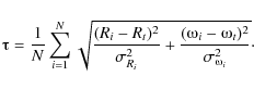
Here, Ri and
![\begin{figure}
\par\includegraphics[width=8.5cm,clip]{9692f1.ps}
\end{figure}](/articles/aa/full_html/2009/20/aa09692-08/img29.png) |
Figure 1:
The rotation curve fitted with solar parameters R0=8.0 kpc and
|
| Open with DEXTER | |
![\begin{figure}
\par\includegraphics[angle=270,width=8.5cm,clip]{9692f2a.ps}\par\includegraphics[angle=270,width=8.5cm,clip]{9692f2b.ps}
\end{figure}](/articles/aa/full_html/2009/20/aa09692-08/img30.png) |
Figure 2:
The distribution of excitation parameters of the HII regions ( top panel) and masses of molecular clouds ( bottom panel). The rotation curve with R0 = 8.5 kpc and |
| Open with DEXTER | |
![\begin{figure}
\par\mbox{\includegraphics[width=8.5cm,clip]{9692f3a.ps}\includeg...
...,clip]{9692f3c.ps}\includegraphics[width=8.5cm,clip]{9692f3d.ps} }\end{figure}](/articles/aa/full_html/2009/20/aa09692-08/img32.png) |
Figure 3:
Panel (1) is the distribution of HII regions, Panel (2) is the distribution of GMCs, and Panel (3) is the distribution of HII regions and GMCs together for illustration of the Galactic spiral structure. The solar parameters R0 = 8.5 kpc and |
| Open with DEXTER | |
More and more pieces of evidence of R0 = 8.0 kpc and ![]() = 220 km s-1 have been found (Eisenhauer et al. 2003; Reid 1993; Groenewegen et al. 2008; Gillessen et al. 2009; Ghez et al. 2008). The change of these constants may affect the kinematic distances of tracers and then affect the derived structure of the Milky Way. Therefore, we fit a new rotation curve with (see Brand & Blitz 1993, R03):
= 220 km s-1 have been found (Eisenhauer et al. 2003; Reid 1993; Groenewegen et al. 2008; Gillessen et al. 2009; Ghez et al. 2008). The change of these constants may affect the kinematic distances of tracers and then affect the derived structure of the Milky Way. Therefore, we fit a new rotation curve with (see Brand & Blitz 1993, R03):
We set the rotation curve to pass through the new R0 and
2.3 Tracers of Galactic spiral structure: weights
The brighter the HII region, the better it is as a tracer of spiral structure. We use the excitation parameters of HII regions as a weighting factor to demonstrate spiral structure. Georgelin & Georgelin (1976) delineated four arm-segments using HII regions with an excitation parameter U greater than 70 pc cm-2. R03 used the excitation parameter as a weighting factor in their fitting process. The excitation parameter U (in pc cm-2) is defined as (Schraml & Mezger 1969):
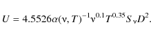
Here, T is the temperature (in K),
Massive molecular clouds are more concentrated to in the spiral arms than clouds with low masses. The mass of a molecular cloud
![]() was rescaled with newly adopted distances. The distribution of
was rescaled with newly adopted distances. The distribution of
![]() is shown in Fig. 2, ranging from 1
is shown in Fig. 2, ranging from 1 ![]()
![]() to 2.5
to 2.5 ![]()
![]() .
More clouds have a lower mass.
.
More clouds have a lower mass.
In order to use the HII regions and GMCs together to outline the spiral structure of our Galaxy, a reasonable match of weighting parameters should be considered to measure their relative importance to the spiral structure. Obviously, a HII region with a higher excitation parameter or a
GMC with a larger
![]() should have a larger value of weight. For the HII regions, we take the weighting parameter B = U/(100 pc cm-2), so that an HII region with U = 100 pc cm-2 has a weight of 1 in the determination of the spiral pattern, while an HII region with U = 200 pc cm-2 has a weight of 2. For the GMCs, the weighting parameter is taken to be
should have a larger value of weight. For the HII regions, we take the weighting parameter B = U/(100 pc cm-2), so that an HII region with U = 100 pc cm-2 has a weight of 1 in the determination of the spiral pattern, while an HII region with U = 200 pc cm-2 has a weight of 2. For the GMCs, the weighting parameter is taken to be
![]() ,
so that the clouds with a mass of
,
so that the clouds with a mass of
![]() have a weight of B=1, and clouds of
have a weight of B=1, and clouds of
![]() have a weight of 2. We have also tried other weighting measures, such as B = U/(50 pc cm-2) and B =
have a weight of 2. We have also tried other weighting measures, such as B = U/(50 pc cm-2) and B =
![]() /
/
![]() ), and found that the arm structure is similar but with more emphasis on GMCs.
), and found that the arm structure is similar but with more emphasis on GMCs.
An additional factor needed in the spiral fitting is the distance uncertainty of each tracer. If the uncertainty of observed stellar distance is known, we use it directly. If the kinematic distance is used, we adopt a systemic velocity uncertainty of ![]() 5 km s-1, and then the distance uncertainty can be derived by using a rotation curve. As we search for the best match of spiral arms in X-Y coordinates, distance uncertainty will be expressed in X and Y. We set a fitting weighting factor
5 km s-1, and then the distance uncertainty can be derived by using a rotation curve. As we search for the best match of spiral arms in X-Y coordinates, distance uncertainty will be expressed in X and Y. We set a fitting weighting factor
![]() and
and
![]() .
We assign all tracers with a
distance accuracy better than 0.5 kpc (i.e.
.
We assign all tracers with a
distance accuracy better than 0.5 kpc (i.e.
![]() kpc) to have wx=1, and wy=1 if
kpc) to have wx=1, and wy=1 if
![]() kpc.
kpc.
Table 1:
The parameters of the best fitting models: the initial radius, Ri, the start azimuthal angle,
![]() ,
and the pitch angle,
,
and the pitch angle,
![]() ,
for the ith arm.
,
for the ith arm.
3 The spiral arms of the Milky Way
Figure 3 shows the distribution of tracers for the Galactic spiral structure projected onto the Galactic plane. The sizes of symbols have been scaled according to the weighting factors B obtained from excitation parameter U or cloud mass. GMCs in a large region of the fourth Galactic quadrant have been mapped by Dame et al. (2001), but unfortunately, the discrete
GMCs have not been identified and explicitly listed in the literature. To show spiral arms better using available data of HII regions and GMCs, in the fourth panel of Fig. 3, we use a Gaussian function to brighten each tracer through:
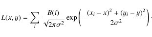
Here we took
![\begin{figure}
\par\includegraphics[width=8.5cm,clip]{9692f4.ps}
\end{figure}](/articles/aa/full_html/2009/20/aa09692-08/img72.png) |
Figure 4:
The spiral structure of HII regions and GMCs (R0=8.5 kpc and
|
| Open with DEXTER | |
In Fig. 4, we overlay our data onto the HI map of Levine et al. (2006), which was obtained with the solar parameters of R0=8.5 kpc,
![]() km s-1. In the HI distribution, there are 3 obvious arm-like structures in the third and fourth quadrants. The Carina arm overlaps with the most inner arm-like structure in the HI distribution, and the Perseus arm may be linked to the intermediate arm-like structure, which can be matched in our 3-arm, 4-arm, and polynomial logarithmic arm models. The counterpart for the outer arm-like structure in the HI map is difficult to identify, but most likely there are one or two spiral arms beyond the Perseus arm.
km s-1. In the HI distribution, there are 3 obvious arm-like structures in the third and fourth quadrants. The Carina arm overlaps with the most inner arm-like structure in the HI distribution, and the Perseus arm may be linked to the intermediate arm-like structure, which can be matched in our 3-arm, 4-arm, and polynomial logarithmic arm models. The counterpart for the outer arm-like structure in the HI map is difficult to identify, but most likely there are one or two spiral arms beyond the Perseus arm.
It is not clear whether the spiral structure of the Milky Way is of logarithmic nature. Canonically, the two, three or four logarithmic arms have been used to fit the tracer data and to model the grand design of our Galaxy. We will try to fit these conventional models to the data, and we also present the polynomial logarithmic arm model with varying pitch angle. In addition to fitting the model to the tracer distribution, it is important to compare the tangential directions of modelled spiral arms to the observed tangents (see Bronfman 1992; Vallée 2008; Englmaier & Gerhard 1999).
In Sect. 3.3, we also show the distribution of tracers for spiral arms by taking the kinematic distances estimated by using the rotation curves with two sets of solar parameters, R0=8.0 kpc and
![]() km s-1 and the recent determination of R0=8.4 kpc and
km s-1 and the recent determination of R0=8.4 kpc and
![]() km s-1 from Reid et al. (2009).
km s-1 from Reid et al. (2009).
![\begin{figure}
\par\includegraphics[width=8.7cm,clip]{9692f5a.ps}\par\includegra...
...clip]{9692f5b.ps}\par\includegraphics[width=8.7cm,clip]{9692f5c.ps}
\end{figure}](/articles/aa/full_html/2009/20/aa09692-08/img73.png) |
Figure 5:
The distribution of HII regions and GMCs (R0=8.5 kpc and
|
| Open with DEXTER | |
3.1 The logarithmic arm models
The logarithmic-arm model describes the ith spiral arm with:
 |
(5) |
Here, r,
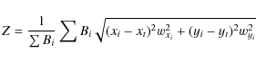
for all tracers; here xi and yi are Cartesian coordinates of the tracer, xt and yt are the coordinates of the nearest point from all spiral arms to the tracer. wxi and wyi are weighting factors for the location uncertainty of xi and yi, respectively, and Bi is the weighting factor related to the excitation parameters of HII regions or the masses of GMCs. The best spiral arm model should be able to minimize the parameter Z.
We assume that each arm always has its own pitch angle in the 2-, 3-, 4-arm models and fit them to the data (see also Naoz & Shaviv 2007). By searching for the best parameters of each arm, Ri,
![]() and
and
![]() in reasonable ranges, to find the minimized Z, we obtained the best spiral arm models as listed in Table 1. Three best-fitting models together with the data are plotted in Fig. 5. The tangential directions of arms in all models are listed in Table 2.
in reasonable ranges, to find the minimized Z, we obtained the best spiral arm models as listed in Table 1. Three best-fitting models together with the data are plotted in Fig. 5. The tangential directions of arms in all models are listed in Table 2.
The best fitting two-arm logarithmic model places the Sun in the Carina arm, and it also connects the Local arm and the Perseus arm with the Carina arm, which is inconsistent with observations. In fact, the connection of the Sagittarius arm and the Carina arm as a single arm has been well established from observations. Such a connection cannot be obtained in any two-arm model, as found by R03. In addition, the tangential directions calculated from this model are also very different from observed values. The parameter Z is slightly larger than that of the 3- and 4-arm models. The best two-arm logarithmic model can be excluded, conclusively.
In the best fitting 3-arm and 4-arm models, the Sagittarius arm and the Carina arm are connected and look very similar. The Scutum arm in the 1st Galactic quadrant outlined by HII regions and molecular clouds is connected to the Crux arm in the 4th Galactic quadrant. This arm is well fitted by
both the 3-arm and the 4-arm models. However, the obvious difference arises from the extension of the Crux arm. It connects to the Perseus+1 arm in the 3-arm model, but to the Perseus+2 arm in the the 4-arm model. It is not clear from current available data whether there is one arm or two arms in the few kpc outside the Perseus arm. Conservatively, the 3-arm model predicts only one Perseus+1 arm and no Perseus+2 arm, which may be more realistic. However, Levine et al. (2006) showed that the HI gas distribution indicates that both the Perseus+1 arm and Perseus+2 arm are possible. The molecular clouds at
![]() at 13 kpc (Digel et al. 1990) may be related to the Perseus+2 arm. In the GC direction, the Norma arm is connected to the Perseus arm in the 3-arm model. In the 4-arm model, the Norma arm is connected to the Perseus+1 arm, and the Perseus arm starts from another arm
inside the Norma arm, corresponding to the Norma-Cygnus arm in the four-arm model of R03.
at 13 kpc (Digel et al. 1990) may be related to the Perseus+2 arm. In the GC direction, the Norma arm is connected to the Perseus arm in the 3-arm model. In the 4-arm model, the Norma arm is connected to the Perseus+1 arm, and the Perseus arm starts from another arm
inside the Norma arm, corresponding to the Norma-Cygnus arm in the four-arm model of R03.
The tangential directions of arms in models are listed in Table 2 for comparison with observations. The double values of the Scutum tangent correspond to both the Scutum arm and another interior arm segment, which can be well fitted in our 3-arm and 4-arm models. However an obvious deviation is seen from the tangent of the actual Scutum arm (
![]() vs.
vs.
![]() ). The tangent of the Sagittarius arm always deviates from observed values by
). The tangent of the Sagittarius arm always deviates from observed values by
![]() or
or
![]() in the 3-arm or the 4-arm model. The tangent of the Norma arm differs by
in the 3-arm or the 4-arm model. The tangent of the Norma arm differs by
![]() in the 4-arm models.
in the 4-arm models.
3.2 The polynomial logarithmic arm model
Note that these spiral arm models are assumed to be purely logarithmic. However, the pitch angle of spiral arms can vary along the arm (see e.g. Seigar & James 1998). If so, a polynomial logarithmic arm model may be necessary to fit both the distribution and tangential directions.
Table 2: Tangential directions from observations (Bronfman 1992; Englmaier & Gerhard 1999) and the best fitting models.
![\begin{figure}
\par\includegraphics[angle=270,width=8.5cm,clip]{9692f6.ps}
\end{figure}](/articles/aa/full_html/2009/20/aa09692-08/img82.png) |
Figure 6:
The distribution of tracer data (R0=8.5 kpc and
|
| Open with DEXTER | |
![\begin{figure}
\par\includegraphics[width=8.7cm,clip]{9692f7a.ps}
\includegraphics[width=8.7cm,clip]{9692f7b.ps}
\end{figure}](/articles/aa/full_html/2009/20/aa09692-08/img83.png) |
Figure 7:
The best-fitting polynomial logarithmic-arm model (R0=8.5 kpc and
|
| Open with DEXTER | |
![\begin{figure}
\par\includegraphics[angle=270,width=8.5cm,clip]{9692f8.ps}
\end{figure}](/articles/aa/full_html/2009/20/aa09692-08/img84.png) |
Figure 8:
The pitch angle ( |
| Open with DEXTER | |
We first plotted the tracer data in the
![]() diagram (see Fig. 6), and roughly identified arm-like features and then separated the data by the dashed-lines. The Sagittarius-Carina arm is very prominent in the plot, which obviously separated in the tracer data from the other groups. The Scutum-Crux arm are also well-isolated in the tracer data, except for those at small r where the data are mixed with those from the Sagittarius arm. The innermost arm seems clearly to have a group of tracers, which in fact is the Norma arm and connected to the Scutum arm. However, outside the Sagittarius-Carina arm, the data are well mixed, and one can barely distinguish the Perseus arm and the Perseus+1 arm, which can only be separated manually in a very rough manner.
diagram (see Fig. 6), and roughly identified arm-like features and then separated the data by the dashed-lines. The Sagittarius-Carina arm is very prominent in the plot, which obviously separated in the tracer data from the other groups. The Scutum-Crux arm are also well-isolated in the tracer data, except for those at small r where the data are mixed with those from the Sagittarius arm. The innermost arm seems clearly to have a group of tracers, which in fact is the Norma arm and connected to the Scutum arm. However, outside the Sagittarius-Carina arm, the data are well mixed, and one can barely distinguish the Perseus arm and the Perseus+1 arm, which can only be separated manually in a very rough manner.
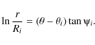
The best model should satisfy the observed tangential directions and also minimize the parameter Z. We separate our total sample into several sub-samples for five arms (see Fig. 6), and fit them separately with the polynomial logarithmic arm model:
| (7) |
to obtain the initial values of each arm, and finally we fit all arms together to the whole sample of data. After using the weighting factors, and minimizing the residual value by Eq. (6), we obtained the best model with the fitting parameters listed in Table 3. The data and arms are plotted in Fig. 7. The tangential directions of this model are also listed in Table 2.
In this model, almost all tracers are best connected with the outlined spiral arms. Compared to the pure logarithmic models, the polynomial logarithmic arm model is more conservative in connecting known tracers. It does not outline the possible arm trajectory in the regions without tracers and predict the possible connection between the outer arms and inner arms. As seen in Fig. 7, the main spiral structures are well traced. From the center we find arm-1 to arm-5, which correspond to the Norma arm, the Scutum-Crux arm, the Sagittarius-Carina arm, the Perseus arm and the Perseus+1 arm. Looking at the HI data in Fig. 4, one may see that arm-5, i.e. the Perseus+1 arm, seems to be connected to the obvious outer HI arm outlined by Levine et al. (2006) at the both ends at about (x,y) = (-12 kpc, +12 kpc) and (+8 kpc, +10 kpc). The Perseus arm is probably connected to the long HI arm at (-12 kpc, +3 kpc). The tangential directions of this model (Table 2) are more consistent with the observed values than those from the logarithmic arm model. We conclude that such a polynomial arm model is a better description of the observed arm features.
The pitch angles of spiral arms vary in the form of
![]() ,
in contrast to the constant pitch angles for the pure logarithmic arms. The pitch angles vary with azimuthal angle, as shown in Fig. 8. Variable pitch angles have been found in nearby
galaxies. For example, Puerari & Dottori (1992) used a simple model with a variable pitch angle to obtain the leading or trailing character of the arms of some galaxies. Note, however, that the innermost segments of arm-2 (
,
in contrast to the constant pitch angles for the pure logarithmic arms. The pitch angles vary with azimuthal angle, as shown in Fig. 8. Variable pitch angles have been found in nearby
galaxies. For example, Puerari & Dottori (1992) used a simple model with a variable pitch angle to obtain the leading or trailing character of the arms of some galaxies. Note, however, that the innermost segments of arm-2 (
![]() )
and arm-3 (
)
and arm-3 (
![]() ), probably due to the distance uncertainty of tracers, show unreasonable negative pitch angles in Fig. 8, similar to the possible outer HI arm (
), probably due to the distance uncertainty of tracers, show unreasonable negative pitch angles in Fig. 8, similar to the possible outer HI arm (![]() kpc) in the 1st quadrant as shown in Fig. 4. This is obtained from tracer data, which thus needs to be resolved.
kpc) in the 1st quadrant as shown in Fig. 4. This is obtained from tracer data, which thus needs to be resolved.
Table 3: The parameters of the polynomial logarithmic arm model.
![\begin{figure}
\par\includegraphics[width=8.7cm,clip]{9692f9a.ps}\par\includegraphics[width=8.7cm,clip]{9692f9b.ps}
\end{figure}](/articles/aa/full_html/2009/20/aa09692-08/img90.png) |
Figure 9:
The best-fitting polynomial logarithmic-arm model for R0=8.0 kpc and
|
| Open with DEXTER | |
![\begin{figure}
\par\includegraphics[width=8.7cm,clip]{9692f10a.ps}\par\includegraphics[width=8.7cm,clip]{9692f10b.ps}
\end{figure}](/articles/aa/full_html/2009/20/aa09692-08/img91.png) |
Figure 10:
The same as Fig. 9 but with the rotation curve from Reid et al. (2009) with R0=8.4 kpc and
|
| Open with DEXTER | |
3.3 The influence of the solar parameters R0 and

We also have re-estimated the distances of HII regions and GMCs, if not available from other measurements, by using the rotation curve for R0=8.0 kpc and
![]() km s-1. Then the excitation parameters of HII regions and the masses of GMCs are accordingly recalculated, as listed in Tables A.1 and A.2. The final distribution of the tracers is shown in Fig. 9. The overall design is similar to that of R0=8.5 kpc and
km s-1. Then the excitation parameters of HII regions and the masses of GMCs are accordingly recalculated, as listed in Tables A.1 and A.2. The final distribution of the tracers is shown in Fig. 9. The overall design is similar to that of R0=8.5 kpc and
![]() km s-1. We also fit the distribution with two, three, and four spiral-arm models, and the parameter values from the best models are listed in Table 1. The best fit of a polynomial logarithmic arm model for a spiral structure is presented in Fig. 9, and the parameters are listed in Table 3. The number of arms and arm structure are conserved. As occured for the case of 8.5/220, the tangential directions are better reproduced by the polynomial model than the logarithmic spiral arm models.
km s-1. We also fit the distribution with two, three, and four spiral-arm models, and the parameter values from the best models are listed in Table 1. The best fit of a polynomial logarithmic arm model for a spiral structure is presented in Fig. 9, and the parameters are listed in Table 3. The number of arms and arm structure are conserved. As occured for the case of 8.5/220, the tangential directions are better reproduced by the polynomial model than the logarithmic spiral arm models.
Reid et al. (2009) used the newly measured trigonometric parallaxes of masers to estimate the solar parameters, and concluded that R0=8.4 ![]() 0.6 kpc and
0.6 kpc and
![]()
![]() 16 km s-1. They offer a revised prescription (and a Fortran code) to calculate kinematic distances and their uncertainties (see Reid et al. 2009, for details). Using the code they kindly provided to us, we determined the kinematic distances and re-scaled other parameters of our HII regions and GMC samples. Their distribution and the best-fitted polynomial logarithmic-arm model is shown in Fig. 10. Compared with the distribution with R0=8.5 kpc and
16 km s-1. They offer a revised prescription (and a Fortran code) to calculate kinematic distances and their uncertainties (see Reid et al. 2009, for details). Using the code they kindly provided to us, we determined the kinematic distances and re-scaled other parameters of our HII regions and GMC samples. Their distribution and the best-fitted polynomial logarithmic-arm model is shown in Fig. 10. Compared with the distribution with R0=8.5 kpc and
![]() km s-1, the tracers are nearer to our sun in the second and third Galactic quadrants, so that arms in this region are wound more tightly. The local arm becomes clearer, but the separation between the Perseus arm and Perseus+1 becomes less clear. The grand design of spiral arms in the other parts of the Galaxy looks very similar to that of 8.0/220.
km s-1, the tracers are nearer to our sun in the second and third Galactic quadrants, so that arms in this region are wound more tightly. The local arm becomes clearer, but the separation between the Perseus arm and Perseus+1 becomes less clear. The grand design of spiral arms in the other parts of the Galaxy looks very similar to that of 8.0/220.
4 Conclusions and remarks
We collected the spiral tracer data of HII regions and giant molecular clouds (GMCs) published in the literature, and used them to study the weighted distribution of these tracers for the overall design of spiral arms of our Milky Way Galaxy. The mass of the GMC and the excitation parameter
of an HII region are scaled as the weighting factors. The distances of tracers, if not available from stellar or triangulation measurements, were estimated kinetically using the rotation curve of BB93 with solar constants of R0=8.5 kpc and
![]() km s-1. We fitted the distribution of these tracers with two, three, and four logarithmic spiral arm models. None of the models can match all the main arm features observed. We finally fit the tracer data by using a polynomial logarithmic arm model, which not only can fit the distribution of tracers for the main spiral arms, but also match the tangential directions with the observations. The polynomial model appears to be better able to describe the spiral arms of our Galaxy. When the kinematic distances are estimated by using rotation curves with two sets of parameters, R0=8.0 kpc and
km s-1. We fitted the distribution of these tracers with two, three, and four logarithmic spiral arm models. None of the models can match all the main arm features observed. We finally fit the tracer data by using a polynomial logarithmic arm model, which not only can fit the distribution of tracers for the main spiral arms, but also match the tangential directions with the observations. The polynomial model appears to be better able to describe the spiral arms of our Galaxy. When the kinematic distances are estimated by using rotation curves with two sets of parameters, R0=8.0 kpc and
![]() km s-1 and R0=8.4 kpc and
km s-1 and R0=8.4 kpc and
![]() km s-1, the distribution
of HII regions and GMCs are slightly better fitted by the models, though the parameters do not change significantly.
km s-1, the distribution
of HII regions and GMCs are slightly better fitted by the models, though the parameters do not change significantly.
For most of tracers in our work, we use their kinematic distances derived from the rotation curves. Gómez (2006) found that the error bars are significantly large for objects at the positions of spiral arms. This pitfall cannot be overcome until accurate distances of a large sample of HII regions are measured, e.g. by triangulation of radio masers (e.g. Reid et al. 2009; Xu et al. 2006). A large project is being carried out with the VLBA to directly measure distances of a large sample of massive star formation regions by trigonometric parallaxes (see Reid et al. 2008) with accuracies approaching
![]() as. Published results of several examples show systematically smaller distances than the kinematic distances. They will probably obtain hundreds of measurements over 10 years for the brightest HII regions covering all the Galactic disk, and the final grand design of our Milky Way will be greatly improved. However, at present, the picture shown in Fig. 10 is the best approximate description of Galactic spiral structure.
as. Published results of several examples show systematically smaller distances than the kinematic distances. They will probably obtain hundreds of measurements over 10 years for the brightest HII regions covering all the Galactic disk, and the final grand design of our Milky Way will be greatly improved. However, at present, the picture shown in Fig. 10 is the best approximate description of Galactic spiral structure.
Acknowledgements
We thank the referee for instructive comments, and Dr. Mark Reid for providing the Fortran code for the estimation of kinematic distances using their newly determined rotation curves. The authors are supported by the National Natural Science Foundation (NNSF) of China (10773016, 10821061 and 10833003) and the National Key Basic Research Science Foundation of China (2007CB815403).
References
- Anderson, L. D., & Bania, T. M. 2009, ApJ, 690, 706 [NASA ADS] [CrossRef]
- Araya, E., Hofner, P., Churchwell, E., & Kurtz, S. 2002, ApJS, 138, 63 [NASA ADS] [CrossRef] (In the text)
- Blum, R. D., Damineli, A., & Conti, P. S. 2001, AJ, 121, 3149 [NASA ADS] [CrossRef]
- Brand, J., & Blitz, L. 1993, A&A, 275, 67 [NASA ADS] (In the text)
- Brand, J., & Wouterloot, J. G. A. 1994, A&AS, 103, 503 [NASA ADS] (In the text)
- Bronfman, L. 1992, in The center, bulge, and disk of the Milky Way, ed. L. Blitz, Astrophys. Space Sci. Libr., 180, 131
- Brunthaler, A., Reid, M. J., Menten, K. M., et al. 2008, ApJ, submitted [arXiv:0811.0713]
- Carpenter, J. M., Snell, R. L., & Schloerb, F. P. 1990, ApJ, 362, 147 [NASA ADS] [CrossRef] (In the text)
- Caswell, J. L., & Haynes, R. F. 1987, A&A, 171, 261 [NASA ADS] (In the text)
- Clemens, D. P. 1985, ApJ, 295, 422 [NASA ADS] [CrossRef] (In the text)
- Cohen, R. S., Dame, T. M., & Thaddeus, P. 1986, ApJS, 60, 695 [NASA ADS] [CrossRef] (In the text)
- Condon, J. J., Cotton, W. D., Greisen, E. W., et al. 1998, AJ, 115, 1693 [NASA ADS] [CrossRef]
- Copetti, M. V. F., Oliveira, V. A., Riffel, R., Castañeda, H. O., & Sanmartim, D. 2007, A&A, 472, 847 [NASA ADS] [CrossRef] [EDP Sciences]
- Crowther, P. A., & Furness, J. P. 2008, A&A, 492, 111 [NASA ADS] [CrossRef] [EDP Sciences]
- Dame, T. M., Elmegreen, B. G., Cohen, R. S., & Thaddeus, P. 1986, ApJ, 305, 892 [NASA ADS] [CrossRef] (In the text)
- Dame, T. M., Hartmann, D., & Thaddeus, P. 2001, ApJ, 547, 792 [NASA ADS] [CrossRef] (In the text)
- Dawson, J. R., Kawamura, A., Mizuno, N., Onishi, T., & Fukui, Y. 2008, PASJ, 60, 1297 [NASA ADS]
- Digel, S., Thaddeus, P., & Bally, J. 1990, ApJ, 357, L29 [NASA ADS] [CrossRef] (In the text)
- Digel, S., de Geus, E., & Thaddeus, P. 1994, ApJ, 422, 92 [NASA ADS] [CrossRef]
- Digel, S. W., Lyder, D. A., Philbrick, A. J., Puche, D., & Thaddeus, P. 1996, ApJ, 458, 561 [NASA ADS] [CrossRef]
- Downes, D., Wilson, T. L., Bieging, J., & Wink, J. 1980, A&AS, 40, 379 [NASA ADS] (In the text)
- Eisenhauer, F., Schödel, R., Genzel, R., et al. 2003, ApJ, 597, L121 [NASA ADS] [CrossRef]
- Englmaier, P., & Gerhard, O. 1999, MNRAS, 304, 512 [NASA ADS] [CrossRef] (In the text)
- Fich, M., Blitz, L., & Stark, A. A. 1989, ApJ, 342, 272 [NASA ADS] [CrossRef] (In the text)
- Fish, V. L., Reid, M. J., Wilner, D. J., & Churchwell, E. 2003, ApJ, 587, 701 [NASA ADS] [CrossRef] (In the text)
- Georgelin, Y. M., & Georgelin, Y. P. 1976, A&A, 49, 57 [NASA ADS] (In the text)
- Ghez, A. M., Salim, S., Weinberg, N. N., et al. 2008, ApJ, 689, 1044 [NASA ADS] [CrossRef]
- Gillessen, S., Eisenhauer, F., Trippe, S., et al. 2009, ApJ, 692, 1075 [NASA ADS] [CrossRef]
- Gómez, G. C. 2006, AJ, 132, 2376 [NASA ADS] [CrossRef] (In the text)
- Grabelsky, D. A., Cohen, R. S., Bronfman, L., & Thaddeus, P. 1988, ApJ, 331, 181 [NASA ADS] [CrossRef] (In the text)
- Gregory, P. C., Scott, W. K., Douglas, K., & Condon, J. J. 1996, ApJS, 103, 427 [NASA ADS] [CrossRef]
- Griffith, M. R., Wright, A. E., Burke, B. F., & Ekers, R. D. 1994, ApJS, 90, 179 [NASA ADS] [CrossRef]
- Griffith, M. R., Wright, A. E., Burke, B. F., & Ekers, R. D. 1995, ApJS, 97, 347 [NASA ADS] [CrossRef]
- Groenewegen, M. A. T., Udalski, A., & Bono, G. 2008, A&A, 481, 441 [NASA ADS] [CrossRef] [EDP Sciences]
- Heyer, M. H., Carpenter, J. M., & Snell, R. L. 2001, ApJ, 551, 852 [NASA ADS] [CrossRef] (In the text)
- Kolpak, M. A., Jackson, J. M., Bania, T. M., Clemens, D. P., & Dickey, J. M. 2003, ApJ, 582, 756 [NASA ADS] [CrossRef] (In the text)
- Kuchar, T. A., & Bania, T. M. 1994, ApJ, 436, 117 [NASA ADS] [CrossRef] (In the text)
- Leahy, D. A., & Tian, W. W. 2008, AJ, 135, 167 [NASA ADS] [CrossRef]
- Levine, E. S., Blitz, L., & Heiles, C. 2006, Science, 312, 1773 [NASA ADS] [CrossRef] (In the text)
- May, J., Alvarez, H., & Bronfman, L. 1997, A&A, 327, 325 [NASA ADS] (In the text)
- Mead, K. N., & Kutner, M. L. 1988, ApJ, 330, 399 [NASA ADS] [CrossRef] (In the text)
- Moscadelli, L., Reid, M. J., Menten, K. M., et al. 2008, ApJ, submitted [arXiv:0811.0679]
- Nakagawa, M., Onishi, T., Mizuno, A., & Fukui, Y. 2005, PASJ, 57, 917 [NASA ADS] (In the text)
- Naoz, S., & Shaviv, N. J. 2007, New Astron., 12, 410 [NASA ADS] [CrossRef] (In the text)
- Paladini, R., Burigana, C., Davies, R. D., et al. 2003, A&A, 397, 213 [NASA ADS] [CrossRef] [EDP Sciences] (In the text)
- Paladini, R., Davies, R. D., & DeZotti, G. 2004, MNRAS, 347, 237 [NASA ADS] [CrossRef] (In the text)
- Pandian, J. D., Momjian, E., & Goldsmith, P. F. 2008, A&A, 486, 191 [NASA ADS] [CrossRef] [EDP Sciences] (In the text)
- Puerari, I., & Dottori, H. A. 1992, A&AS, 93, 469 [NASA ADS] (In the text)
- Reid, M. J. 1993, ARA&A, 31, 345 [NASA ADS] [CrossRef]
- Reid, M. J., Menten, K. M., Brunthaler, A., et al. 2008, ApJ, submitted [arXiv:0811.0595]
- Reid, M. J., Menten, K. M., Zheng, X. W., et al. 2009, ApJ, submitted [arXiv:0902.3913] (In the text)
- Russeil, D. 2003, A&A, 397, 133 [NASA ADS] [CrossRef] [EDP Sciences] (In the text)
- Russeil, D., Adami, C., & Georgelin, Y. M. 2007, A&A, 470, 161 [NASA ADS] [CrossRef] [EDP Sciences] (In the text)
- Schraml, J., & Mezger, P. G. 1969, ApJ, 156, 269 [NASA ADS] [CrossRef] (In the text)
- Seigar, M. S., & James, P. A. 1998, MNRAS, 299, 685 [NASA ADS] [CrossRef] (In the text)
- Sewilo, M., Watson, C., Araya, E., et al. 2004, ApJS, 154, 553 [NASA ADS] [CrossRef] (In the text)
- Sodroski, T. J. 1991, ApJ, 366, 95 [NASA ADS] [CrossRef] (In the text)
- Solomon, P. M., Rivolo, A. R., Barrett, J., & Yahil, A. 1987, ApJ, 319, 730 [NASA ADS] [CrossRef] (In the text)
- Tian, W. W., & Leahy, D. A. 2008, ApJ, 677, 292 [NASA ADS] [CrossRef]
- Tian, W. W., Li, Z., Leahy, D. A., & Wang, Q. D. 2007, ApJ, 657, L25 [NASA ADS] [CrossRef]
- Tian, W. W., Leahy, D. A., Haverkorn, M., & Jiang, B. 2008, ApJ, 679, L85 [NASA ADS] [CrossRef]
- Vallée, J. P. 2008, AJ, 135, 1301 [NASA ADS] [CrossRef] (In the text)
- Watson, C., Araya, E., Sewilo, M., et al. 2003, ApJ, 587, 714 [NASA ADS] [CrossRef] (In the text)
- Wright, A. E., Griffith, M. R., Burke, B. F., & Ekers, R. D. 1994, ApJS, 91, 111 [NASA ADS] [CrossRef]
- Wright, A. E., Griffith, M. R., Hunt, A. J., et al. 1996, ApJS, 103, 145 [NASA ADS] [CrossRef]
- Xu, Y., Reid, M. J., Zheng, X. W., & Menten, K. M. 2006, Science, 311, 54 [NASA ADS] [CrossRef]
- Xu, Y., Reid, M. J., Menten, K. M., et al. 2008, ApJ, submitted [arXiv:0811.0701]
- Zhang, B., Zheng, X. W., Reid, M. J., et al. 2008, ApJ, submitted [arXiv:0811.0704]
Online Material
Appendix A: Tracer data for spiral structure
We collected and calculated the related parameters of HII regions and giant molecular clouds (GMCs) based on the observations in the literature, and present them here in two tables.
Table A.1:
HII regions as tracers of spiral arms. Columns 1 to 3 list the Galactic longitude, Galactic latitude and velocity, taken from the reference given in Col. 4; Cols. 5 to 7 give the radio continuum flux of the HII region, observation frequency and the reference. Columns 8 to 10 give the stellar distance when available, as well as the error and the reference; Col. 11 is a note for the distance ambiguity and Col. 12 is its reference: Knear - the nearer kinematic distance is adopted; Kfar - the farther kinematic distance is adopted; Ktan - the tracer is located at the tangential point and the distance to the tangent is adopted; Kout - the object is in the outer Galaxy and only one kinematic distance is available and adopted; Cols. 13 and 14 give the kinematic distance to the Sun and distance to the Galactic Center estimated with a rotation curve with R0=8.5 kpc,
![]() km s-1; Col. 15 contains the excitation parameter rescaled by the distance we adopted; Cols. 16 to 18 are the same as Cols. 13-15 but with constants R0=8.0 kpc and
km s-1; Col. 15 contains the excitation parameter rescaled by the distance we adopted; Cols. 16 to 18 are the same as Cols. 13-15 but with constants R0=8.0 kpc and
![]() km s-1 for kinematic distances. Columns 19 to 21 are the same as Cols. 13-15 but with constants R0=8.4 kpc and
km s-1 for kinematic distances. Columns 19 to 21 are the same as Cols. 13-15 but with constants R0=8.4 kpc and
![]() km s-1 for kinematic distances.
km s-1 for kinematic distances.
Table A.2:
GMCs as tracers of spiral arms. Columns 1 and 2 are the Galactic longitude and latitude; Cols. 3 to 6 list velocity, the luminosity of CO emission line (in unit of 103 K km s-1 pc2), distance and mass of molecular cloud, which were all taken from the reference given in Col. 8; Col. 7 is the note for distance ambiguity given in this reference, used as the same convention as in Table A.1; Cols. 9 and 10 list the distances to the Sun and to the Galactic center, which are estimated by the velocity and the rotation curve with R0=8.5 kpc
and
Table 1:
The parameters of the best fitting models: the initial radius, Ri, the start azimuthal angle,
Table 2:
Tangential directions from observations (Bronfman 1992; Englmaier & Gerhard 1999) and the best fitting models.
Table 3:
The parameters of the polynomial logarithmic arm model.
Table A.1:
HII regions as tracers of spiral arms. Columns 1 to 3 list the Galactic longitude, Galactic latitude and velocity, taken from the reference given in Col. 4; Cols. 5 to 7 give the radio continuum flux of the HII region, observation frequency and the reference. Columns 8 to 10 give the stellar distance when available, as well as the error and the reference; Col. 11 is a note for the distance ambiguity and Col. 12 is its reference: Knear - the nearer kinematic distance is adopted; Kfar - the farther kinematic distance is adopted; Ktan - the tracer is located at the tangential point and the distance to the tangent is adopted; Kout - the object is in the outer Galaxy and only one kinematic distance is available and adopted; Cols. 13 and 14 give the kinematic distance to the Sun and distance to the Galactic Center estimated with a rotation curve with R0=8.5 kpc,
Table A.2:
GMCs as tracers of spiral arms. Columns 1 and 2 are the Galactic longitude and latitude; Cols. 3 to 6 list velocity, the luminosity of CO emission line (in unit of 103 K km s-1 pc2), distance and mass of molecular cloud, which were all taken from the reference given in Col. 8; Col. 7 is the note for distance ambiguity given in this reference, used as the same convention as in Table A.1; Cols. 9 and 10 list the distances to the Sun and to the Galactic center, which are estimated by the velocity and the rotation curve with R0=8.5 kpc
and
The rotation curve fitted with solar parameters R0=8.0 kpc and
The distribution of excitation parameters of the HII regions ( top panel) and masses of molecular clouds ( bottom panel). The rotation curve with R0 = 8.5 kpc and ![]() km s-1 when the stellar distance is unavailable; Col. 11 gives the mass of molecular clouds re-scaled by the newly estimated distance; Cols. 12-14 are the same as Cols. 9-11 but with R0=8.0 kpc and
km s-1 when the stellar distance is unavailable; Col. 11 gives the mass of molecular clouds re-scaled by the newly estimated distance; Cols. 12-14 are the same as Cols. 9-11 but with R0=8.0 kpc and
![]() km s-1. Columns 15-17 are the same as Cols. 9-11 but with R0=8.4 kpc and
km s-1. Columns 15-17 are the same as Cols. 9-11 but with R0=8.4 kpc and
![]() km s-1.
km s-1.
Footnotes
![]()
All Tables
![]() ,
and the pitch angle,
,
and the pitch angle,
![]() ,
for the ith arm.
,
for the ith arm.
![]() km s-1; Col. 15 contains the excitation parameter rescaled by the distance we adopted; Cols. 16 to 18 are the same as Cols. 13-15 but with constants R0=8.0 kpc and
km s-1; Col. 15 contains the excitation parameter rescaled by the distance we adopted; Cols. 16 to 18 are the same as Cols. 13-15 but with constants R0=8.0 kpc and
![]() km s-1 for kinematic distances. Columns 19 to 21 are the same as Cols. 13-15 but with constants R0=8.4 kpc and
km s-1 for kinematic distances. Columns 19 to 21 are the same as Cols. 13-15 but with constants R0=8.4 kpc and
![]() km s-1 for kinematic distances.
km s-1 for kinematic distances.
![]() km s-1 when the stellar distance is unavailable; Col. 11 gives the mass of molecular clouds re-scaled by the newly estimated distance; Cols. 12-14 are the same as Cols. 9-11 but with R0=8.0 kpc and
km s-1 when the stellar distance is unavailable; Col. 11 gives the mass of molecular clouds re-scaled by the newly estimated distance; Cols. 12-14 are the same as Cols. 9-11 but with R0=8.0 kpc and
![]() km s-1. Columns 15-17 are the same as Cols. 9-11 but with R0=8.4 kpc and
km s-1. Columns 15-17 are the same as Cols. 9-11 but with R0=8.4 kpc and
![]() km s-1.
km s-1.
All Figures
Figure 1:
![]() km s-1. Data are taken from our collected sample listed in Tables A.1 and A.2.
km s-1. Data are taken from our collected sample listed in Tables A.1 and A.2.Open with DEXTER In the text
Figure 2:
![]() = 220 km s-1 was used if the distances of these tracers were estimated kinetically.
= 220 km s-1 was used if the distances of these tracers were estimated kinetically.Open with DEXTER In the text
| |
Figure 3:
Panel (1) is the distribution of HII regions, Panel (2) is the distribution of GMCs, and Panel (3) is the distribution of HII regions and GMCs together for illustration of the Galactic spiral structure. The solar parameters R0 = 8.5 kpc and |
| Open with DEXTER | |
| In the text | |
| |
Figure 4:
The spiral structure of HII regions and GMCs (R0=8.5 kpc and
|
| Open with DEXTER | |
| In the text | |
| |
Figure 5:
The distribution of HII regions and GMCs (R0=8.5 kpc and
|
| Open with DEXTER | |
| In the text | |
| |
Figure 6:
The distribution of tracer data (R0=8.5 kpc and
|
| Open with DEXTER | |
| In the text | |
| |
Figure 7:
The best-fitting polynomial logarithmic-arm model (R0=8.5 kpc and
|
| Open with DEXTER | |
| In the text | |
| |
Figure 8:
The pitch angle ( |
| Open with DEXTER | |
| In the text | |
| |
Figure 9:
The best-fitting polynomial logarithmic-arm model for R0=8.0 kpc and
|
| Open with DEXTER | |
| In the text | |
| |
Figure 10:
The same as Fig. 9 but with the rotation curve from Reid et al. (2009) with R0=8.4 kpc and
|
| Open with DEXTER | |
| In the text | |
Copyright ESO 2009
Current usage metrics show cumulative count of Article Views (full-text article views including HTML views, PDF and ePub downloads, according to the available data) and Abstracts Views on Vision4Press platform.
Data correspond to usage on the plateform after 2015. The current usage metrics is available 48-96 hours after online publication and is updated daily on week days.
Initial download of the metrics may take a while.