| Issue |
A&A
Volume 499, Number 1, May III 2009
|
|
|---|---|---|
| Page(s) | 191 - 213 | |
| Section | Interstellar and circumstellar matter | |
| DOI | https://doi.org/10.1051/0004-6361/200811511 | |
| Published online | 25 March 2009 | |
Radio emission and nonlinear diffusive shock acceleration of cosmic rays in the supernova SN 1993J
V. Tatischeff
1 - Centre de Spectrométrie Nucléaire et de Spectrométrie de
Masse, CNRS/IN2P3 and Univ Paris-Sud, 91405 Orsay, France![]()
2 - Institut de Ciències de l'Espai (CSIC-IEEC), Campus UAB,
Fac. Ciències, 08193 Bellaterra, Barcelona, Spain
Received 12 December 2008 / Accepted 13 March 2009
Abstract
Aims. The extensive observations of the supernova SN 1993J at radio wavelengths make this object a unique target for the study of particle acceleration in a supernova shock.
Methods. To describe the radio synchrotron emission we use a model that couples a semianalytic description of nonlinear diffusive shock acceleration with self-similar solutions for the hydrodynamics of the supernova expansion. The synchrotron emission, which is assumed to be produced by relativistic electrons propagating in the postshock plasma, is worked out from radiative transfer calculations that include the process of synchrotron self-absorption. The model is applied to explain the morphology of the radio emission deduced from high-resolution VLBI imaging observations and the measured time evolution of the total flux density at six frequencies.
Results. Both the light curves and the morphology of the radio emission indicate that the magnetic field was strongly amplified in the blast wave region shortly after the explosion, possibly via the nonresonant regime of the cosmic-ray streaming instability operating in the shock precursor. The amplified magnetic field immediately upstream from the subshock is determined to be
![]() G. The turbulent magnetic field was not damped behind the shock but carried along by the plasma flow in the downstream region. Cosmic-ray protons were efficiently produced by diffusive shock acceleration at the blast wave. We find that during the first
G. The turbulent magnetic field was not damped behind the shock but carried along by the plasma flow in the downstream region. Cosmic-ray protons were efficiently produced by diffusive shock acceleration at the blast wave. We find that during the first ![]() 8.5 years after the explosion, about 19% of the total energy processed by the forward shock was converted to cosmic-ray energy. However, the shock remained weakly modified by the cosmic-ray pressure. The high magnetic field amplification implies that protons were rapidly accelerated to energies well above 1015 eV. The results obtained for this supernova support the scenario that massive stars exploding into their former stellar wind are a major source of Galactic cosmic-rays of energies above
8.5 years after the explosion, about 19% of the total energy processed by the forward shock was converted to cosmic-ray energy. However, the shock remained weakly modified by the cosmic-ray pressure. The high magnetic field amplification implies that protons were rapidly accelerated to energies well above 1015 eV. The results obtained for this supernova support the scenario that massive stars exploding into their former stellar wind are a major source of Galactic cosmic-rays of energies above ![]() 1015 eV. We also calculate the flux from SN 1993J of gamma-rays arising from collisions of accelerated cosmic rays with ambient material and the result suggests that type II supernovae could be detected in
1015 eV. We also calculate the flux from SN 1993J of gamma-rays arising from collisions of accelerated cosmic rays with ambient material and the result suggests that type II supernovae could be detected in ![]() -decay gamma-rays with the Fermi Gamma-ray Space Telescope out to a maximum distance of only
-decay gamma-rays with the Fermi Gamma-ray Space Telescope out to a maximum distance of only ![]() 1 Mpc.
1 Mpc.
Key words: acceleration of particles - magnetic fields - radiation mechanisms: non-thermal - stars: supernovae: individual: SN 1993J
1 Introduction
Galactic cosmic rays are widely believed to be accelerated in expanding shock waves initiated by supernova (SN) explosions, at least up to the ``knee'' energy of the cosmic-ray spectrum at ![]() 1015 eV and possibly up to the ``ankle'' at
1015 eV and possibly up to the ``ankle'' at ![]() 1018 eV (Axford 1994). The theory of diffusive shock acceleration (DSA) of cosmic rays is well established (see, e.g., Jones & Ellison 1991; Malkov & Drury 2001, for reviews), but two fundamental questions remain partly unanswered by the theory: what is the maximum kinetic energy achieved by particles accelerated in SN shocks and what is the acceleration efficiency, i.e. the fraction of the total SN energy converted to cosmic-ray energy?
1018 eV (Axford 1994). The theory of diffusive shock acceleration (DSA) of cosmic rays is well established (see, e.g., Jones & Ellison 1991; Malkov & Drury 2001, for reviews), but two fundamental questions remain partly unanswered by the theory: what is the maximum kinetic energy achieved by particles accelerated in SN shocks and what is the acceleration efficiency, i.e. the fraction of the total SN energy converted to cosmic-ray energy?
The maximum cosmic-ray energy attainable in a SN shock scales as the product of the shock size and the strength of the turbulent magnetic field in the acceleration region (e.g. Marcowith et al. 2006). Multiwavelength observations of young shell-type supernova remnants (SNRs) provide evidence that the magnetic field in the blast wave region is much higher than the interstellar magnetic field (e.g. Völk et al. 2005; Cassam-Chenaï et al. 2007; Uchiyama et al. 2007, and references therein). A possible explanation for these observations is that the ambient magnetic field is amplified by the diffusive streaming of accelerated particles in the upstream region of the shock, which could cause a plasma instability generating large-amplitude magnetic turbulence
(Bell & Lucek 2001; Amato & Blasi 2006; Vladimirov et al. 2006). Magnetic field amplification via this nonlinear process could facilitate the acceleration of protons in SNRs up to ![]() 1015 eV (e.g. Parizot et al. 2006).
1015 eV (e.g. Parizot et al. 2006).
The acceleration efficiency depends on the diffusive transport of energetic particles at both sides of the shock in the self-generated turbulence (e.g. Malkov & Drury 2001). The DSA theory cannot accurately predict at the present time how many particles are injected into the acceleration process as a function of the shock parameters. Observations of SNRs in high-energy gamma-rays can provide valuable information on the efficiency of cosmic-ray acceleration in these objects. But it remains unclear whether the emission detected from several SNRs with ground-based atmospheric Cherenkov telescopes is due mainly to pion decay following hadronic collisions of accelerated ions or to inverse Compton scattering of ambient photons by accelerated electrons (e.g. Morlino et al. 2008).
However, theory predicts that efficient acceleration of cosmic-ray ions (mainly protons) modifies the shock structure with respect to the case with no acceleration (see, e.g., Berezhko & Ellison 1999). In particular, the total compression ratio of a cosmic-ray-modified shock can be much higher than that of a test-particle shock (i.e. when the accelerated particles have no influence on the shock structure), because relativistic particles produce less pressure for a given energy density than do nonrelativistic particles. In addition, the energy loss due to escape of accelerated cosmic rays from the shock system can further increase the compressibility of the shocked gas (see Decourchelle et al. 2000). Furthermore, since the energy going into relativistic particles is drawn from the shocked-heated thermal population, the postshock temperature of a cosmic-ray-modified shock can be much lower than the test-particle value. Observations of these nonlinear effects (Hughes et al. 2000; Decourchelle 2005; Warren et al. 2005) provide indirect evidence for the efficient acceleration of cosmic-ray protons (which carry most of the total nonthermal particle pressure) in shock waves of young SNRs.
In this paper, we study the production of cosmic-rays by nonlinear DSA and the associated magnetic field amplification in a very young SN shock, which expands in a relatively dense stellar wind lost by the progenitor star prior to explosion. We use radio monitoring observations of SN 1993J conducted with the Very Large Array and several other radio telescopes since the SN outburst (see Weiler et al. 2007; Bartel et al. 2007, and references therein). The radio emission from SNe is thought to be synchrotron radiation from relativistic electrons of energies <1 GeV accelerated at the expanding blast wave (Chevalier 1982b; Fransson & Björnsson 1998). The key motivation for the present study is that the radiating electrons can be influenced by the presence of otherwise unseen shock-accelerated protons. In particular, the theory of nonlinear DSA predicts that the energy distribution of nonthermal electrons below 1 GeV steepens with increasing efficiency of proton acceleration (Ellison et al. 2000).
We chose SN 1993J because it is one of the brightest radio SNe ever detected and has already been the subject of numerous very useful observational and theoretical studies (see, e.g., for the radio emission of SN 1993J Bartel et al. 1994,2000,2007; Marcaide et al. 1994,1995,1997; Van Dyk et al. 1994; Fransson et al. 1996; Fransson & Björnsson 1998; Pérez-Torres et al. 2001; Mioduszewski et al. 2001; Bietenholz et al. 2003; Weiler et al. 2007, and references therein).
The model of the present paper is largely based on the work of Cassam-Chenaï et al. (2005; see also Decourchelle et al. 2000; Ellison & Cassam-Chenaï 2005) on the morphology of synchrotron emission in Galactic SNRs. These authors have developed a model to study radio and X-ray images of SNRs undergoing efficient cosmic-ray production, that couples a semianalytic description of nonlinear DSA with self-similar solutions for the hydrodynamics of the SN expansion. The model has recently been applied to the remnants of Tycho's SN (Cassam-Chenaï et al. 2007) and SN 1006 (Cassam-Chenaï et al. 2008).
Duffy et al. (1995) have studied the radio emission from SN 1987A by considering a two-fluid system consisting of a cosmic-ray gas and a thermal plasma to calculate the structure of the blast wave. In their model, however, the efficiency of cosmic-ray acceleration is not deduced from the radio data, but assumed to be similar to that required in SNRs to explain the observed flux of Galactic cosmic rays. Another difference with the present work is that the turbulent magnetic field in the shock precursor is not assumed to be amplified by the DSA process, but is taken by these authors to be of the same order as the ordered field in the wind of the progenitor star.
A preliminary account of the present work has been given elsewhere (Tatischeff 2008) and all of the present results supersede those published earlier.
2 Model
2.1 Forward shock expansion
The type IIb SN 1993J was discovered in the galaxy M 81 by Garcia (Ripero
et al. 1993) on 1993 March 28, shortly after shock breakout (Wheeler
et al. 1993). Very long baseline interferometry (VLBI) observations (see, e.g., Marcaide et al. 1997; Bietenholz et al. 2003) revealed a decelerating expansion of a shell-like radio source. The radio emission is presumably produced between the forward shock propagating into the circumstellar medium (CSM) and the reverse shock running into the SN ejecta (e.g. Bartel et al. 2007). Marcaide et al. (1997) found the outer angular radius of the radio shell to evolve as a function of time t after explosion with the power law
![]() ,
where the deceleration parameter
,
where the deceleration parameter
![]() .
More recently, Weiler et al. (2007, and references therein) reported that the angular expansion of SN 1993J up to day 1500 after outburst can be expressed as
.
More recently, Weiler et al. (2007, and references therein) reported that the angular expansion of SN 1993J up to day 1500 after outburst can be expressed as
![]()
![]() as with
as with
![]() ;
here
;
here ![]() is by definition the angular radius of the circle that encompasses half of the total radio flux density to better than 20%.
is by definition the angular radius of the circle that encompasses half of the total radio flux density to better than 20%.
These results are consistent with the standard, analytical model for the expansion of a SN into a CSM (Chevalier 1982a,1983; Nadyozhin 1985). This model assumes power-law density profiles for both the outer SN ejecta,
![]() (with n>5), and the CSM,
(with n>5), and the CSM,
![]() (with s<3), where C2 and C1 are constants. The SN expansion is then found to be self-similar (i.e. the structure of the interaction region between the forward and reverse shocks remains constant in time except for a scaling factor) and the deceleration parameter
m=(n-3)/(n-s). For a standard wind density profile with s=2 (see below), the deceleration reported by Weiler et al. (2007) corresponds to
(with s<3), where C2 and C1 are constants. The SN expansion is then found to be self-similar (i.e. the structure of the interaction region between the forward and reverse shocks remains constant in time except for a scaling factor) and the deceleration parameter
m=(n-3)/(n-s). For a standard wind density profile with s=2 (see below), the deceleration reported by Weiler et al. (2007) corresponds to
![]() ,
in fair agreement with numerical computations of SN explosions (e.g. Arnett 1988).
,
in fair agreement with numerical computations of SN explosions (e.g. Arnett 1988).
However, Bartel et al. (2000,2002) found significant changes with time of the parameter m, indicating deviations from a self-similar expansion. These authors determined the outer angular radius
![]() as a function of time by consistently fitting to the two-dimensional radio images observed at 34 epochs between 1993 and 2001 the projection of a three-dimensional spherical shell of uniform volume emissivity. They fixed the ratio of the outer to inner angular radius (as expected from a self-similar expansion) at
as a function of time by consistently fitting to the two-dimensional radio images observed at 34 epochs between 1993 and 2001 the projection of a three-dimensional spherical shell of uniform volume emissivity. They fixed the ratio of the outer to inner angular radius (as expected from a self-similar expansion) at
![]() .
By performing a least-squares power-law fit to the values of
.
By performing a least-squares power-law fit to the values of
![]() thus determined (see Fig. 1), they obtained a minimum reduced
thus determined (see Fig. 1), they obtained a minimum reduced ![]() of
of
![]() for 64 degrees of freedom, indicating that the null hypothesis of a self-similar expansion can be rejected.
for 64 degrees of freedom, indicating that the null hypothesis of a self-similar expansion can be rejected.
As discussed by Bartel et al. (2002), this result strongly depends on the systematic errors associated with the model of uniform emissivity in the spherical shell. The overall systematic uncertainty was estimated to range from 3% at early epochs to 1% at later epochs and to dominate the statistical error in most of the cases. We show below (Sect. 3.1) that the assumption of uniform emissivity is questionable, because radio-emitting electrons accelerated at the forward shock are expected to lose most of their kinetic energy by radiative losses before reaching the contact discontinuity between shocked ejecta and shocked CSM (see also Fransson & Björnsson 1998). Furthermore, the radial emissivity profile is expected to vary with time and radio frequency![]() . Although the systematic uncertainties were carefully studied by Bartel et al. (2002), we note that a moderate increase of the errors would make the expansion compatible with the self-similar assumption. For example, by setting a lower limit of 3% on the uncertainties in the outer radii measured by Bartel et al., we get from a least-squares power-law fit to the data
. Although the systematic uncertainties were carefully studied by Bartel et al. (2002), we note that a moderate increase of the errors would make the expansion compatible with the self-similar assumption. For example, by setting a lower limit of 3% on the uncertainties in the outer radii measured by Bartel et al., we get from a least-squares power-law fit to the data
![]() and an associated probability of chance coincidence of 8%. Thus, the null hypothesis of a self-similar expansion could not anymore be rejected at the usual significance level of 5%.
and an associated probability of chance coincidence of 8%. Thus, the null hypothesis of a self-similar expansion could not anymore be rejected at the usual significance level of 5%.
![\begin{figure}
\par\includegraphics[width=8.8cm]{1511f1.eps}
\end{figure}](/articles/aa/full_html/2009/19/aa11511-08/img68.png) |
Figure 1: Time evolution of the outer angular radius of the shell-like radio emission from SN 1993J. The data were obtained by Bartel et al. (2002) from observations at 1.7, 2.3, 5.0, 8.4, 14.8, and 22.2 GHz. The dotted line is a least-squares power-law fit to the data (Eq. (1)). |
| Open with DEXTER | |
For simplicity, I shall use the self-similar solution to model the hydrodynamic evolution of the SNR (Sect. 2.5). The radius of the forward shock,
![]() where the source distance
where the source distance
![]() Mpc (Freedman et al. 1994), is estimated from a power-law fit to the data of Bartel et al. (2002) at all frequencies (Fig. 1), which gives
Mpc (Freedman et al. 1994), is estimated from a power-law fit to the data of Bartel et al. (2002) at all frequencies (Fig. 1), which gives
Thus, we have
In the self-similar model, the forward shock radius is given by (e.g. Chevalier 1983)
where the constant
where
2.2 Free-free absorption of the radio emission in the circumstellar medium
Figure 2 shows a set of light curves measured for SN 1993J at 0.3 cm (85-110 GHz), 1.2 cm (22.5 GHz), 2 cm (14.9 GHz), 3.6 cm (8.4 GHz), 6 cm (4.9 GHz), and 20 cm (1.4 GHz). We see that at each wavelength the flux density first rapidly increases and then declines more slowly as a power in time (the data at 0.3 cm do not allow to clearly identify this behavior). The radio emission was observed to suddenly decline after day ![]() 3100 (not shown in Fig. 2), which is interpreted in terms of an abrupt decrease of the CSM density at radial distance from the progenitor
3100 (not shown in Fig. 2), which is interpreted in terms of an abrupt decrease of the CSM density at radial distance from the progenitor
![]() cm (Weiler et al. 2007). This is presumably the outer limit of the dense cocoon which was established by a high mass loss from the red supergiant progenitor of the SN for
cm (Weiler et al. 2007). This is presumably the outer limit of the dense cocoon which was established by a high mass loss from the red supergiant progenitor of the SN for ![]() 104 years before explosion.
104 years before explosion.
![\begin{figure}
\par\includegraphics[width=12cm]{1511f2.eps}
\end{figure}](/articles/aa/full_html/2009/19/aa11511-08/img85.png) |
Figure 2: Radio light curves for SN 1993J at 0.3, 1.2, 2, 3.6, 6, and 20 cm. The data are from Weiler et al. (2007) and references therein. The solid lines represent the best-fit semi-empirical model of these authors. The dotted lines show a synchrotron self-absorption (SSA) model in which the SSA optical depth and the unabsorbed flux density were obtained from fits to radio spectra taken between day 75 and day 923 after outburst (see Sect. 2.3). The difference between the latter model and the data before day 100 is partly due to free-free absorption of the radio emission in the CSM. |
| Open with DEXTER | |
We see in Fig. 2 that the maximum intensity is reached first at lower wavelengths and later at higher wavelengths, which is characteristic of absorption processes. For SN 1993J, both free-free absorption (FFA) in the CSM and synchrotron self-absorption (SSA) are important (Chevalier 1998; Fransson & Björnsson 1998; Weiler et al. 2007). The Razin effect can be excluded (Fransson & Björnsson 1998). FFA is produced in the stellar wind that has been heated and ionized by radiation from the shock breakout. If the circumstellar gas is homogeneous and of uniform temperature
![]() ,
the radio emission produced behind the forward shock is typically attenuated by a factor
,
the radio emission produced behind the forward shock is typically attenuated by a factor
![]() ,
where the optical depth at a given frequency
,
where the optical depth at a given frequency ![]() satisfies (Weiler et al. 1986)
satisfies (Weiler et al. 1986)
From a fit to early data using the parametrized model of Weiler et al. (1986,2002; see Appendix A), Van Dyk et al. (1994) found for the time dependance of the optical depth
Fransson & Björnsson (1998) performed the most detailed modeling of the radio emission from SN 1993J to date. In particular, they took into account both FFA and SSA, and included all relevant energy loss mechanisms for the relativistic electrons. As a result, they were able to adequately reproduce the radio light curves with the standard s=2 density profile. In their model, the measured time dependence of the FFA optical depth (i.e. ![]() )
is accounted for by a decrease of
)
is accounted for by a decrease of
![]() with radius like
with radius like
![]() (see also Fransson
et al. 1996). However, as pointed out by Weiler et al. (2002), no evidence for such a radial dependence of
(see also Fransson
et al. 1996). However, as pointed out by Weiler et al. (2002), no evidence for such a radial dependence of
![]() is found in other radio SNe (e.g. SN 1979C and SN 1980K).
is found in other radio SNe (e.g. SN 1979C and SN 1980K).
Immler et al. (2001) provided support from X-ray observations to the scenario of a flatter CSM density profile, as they found s=1.63 from modeling of the observed X-ray light curve. Their analysis assumes that the X-ray emission arises from the forward, circumstellar shock. But later than ![]() 200 days post-outburst, the X-ray radiation was more likely produced in the SN ejecta heated by the reverse shock (Fransson & Björnsson 2005, and references therein).
200 days post-outburst, the X-ray radiation was more likely produced in the SN ejecta heated by the reverse shock (Fransson & Björnsson 2005, and references therein).
With the model of the present paper, the measured radio light curves can be well explained with the standard s=2 assumption, but not with a much flatter CSM density profile. This result is independent of the admittedly uncertain FFA modeling, as we will see in Sect. 4.1 that with s=1.6 the optically thin emission cannot be simultaneously reproduced at all wavelengths in the framework of the model (see Fig. 14). So the question is how a
![]() density profile can be reconciled with the relatively low value of
density profile can be reconciled with the relatively low value of ![]() implied by the data.
implied by the data.
A possible explanation is that the absorbing CSM is inhomogeneous. Both radio (Weiler et al. 1990) and optical and UV (e.g. Tran et al. 1997) observations show that the wind material lost from SN progenitors can be clumpy and/or filamentary. FFA of the radio emission by a nonuniform CSM can be accounted for by an attenuation factor of the form
![]() ,
where
,
where
![]() is the maximum of the optical depth distribution, which depends on the number density and geometric cross section of the clumps of wind material (Natta & Panagia 1984; Weiler et al. 2002). Weiler et al. (2007) performed an overall fit to all of the measured radio light curves of SN 1993J using a parametrized model that takes into account both SSA and FFA, and includes both attenuation by a homogeneous and inhomogeneous CSM (see Appendix A). In their best-fit model (solid lines in Fig. 2), FFA is mainly due to the clumpy CSM, the corresponding optical depth,
is the maximum of the optical depth distribution, which depends on the number density and geometric cross section of the clumps of wind material (Natta & Panagia 1984; Weiler et al. 2002). Weiler et al. (2007) performed an overall fit to all of the measured radio light curves of SN 1993J using a parametrized model that takes into account both SSA and FFA, and includes both attenuation by a homogeneous and inhomogeneous CSM (see Appendix A). In their best-fit model (solid lines in Fig. 2), FFA is mainly due to the clumpy CSM, the corresponding optical depth,
![]() ,
being much larger than
,
being much larger than
![]() in the optically thick phase for all wavelengths (see Table 4 in Weiler et al. 2007).
in the optically thick phase for all wavelengths (see Table 4 in Weiler et al. 2007).
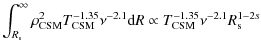
In view of these results, we are going to neglect in first approximation the attenuation of the radio emission by the homogeneous component of the CSM in front of the attenuation by the clumpy CSM, which will allow us to derive in a simple way and self-consistently the mass loss rate of the progenitor star and the structure of the radio emission region (see below). We anticipate, however, that the adopted simple FFA model will not allow us to accurately reproduce the rising branches of the light curves in the optically thick phase.
Following Weiler et al. (1986,2002), the optical depth produced by FFA in a clumpy presupernova wind can be written as
with, for a uniform
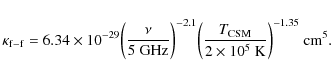
Here,
where we adopted X=0.3 (e.g. Shigeyama et al. 1994). In the following we use uw=10 km s-1 and
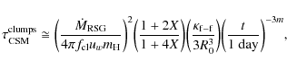
FFA in the progenitor wind of SN 1993J is estimated below from the following iterative process. First the synchrotron emission as a function of time after outburst is calculated from a set of reasonable initial parameters. External FFA is then estimated from an overall fit of the calculated light curves to the radio data, using Eqs. (A.3) and (A.6) for the CSM attenuation factor with fixed
![]() (see Eq. (6)). Thus, the only free parameter is K3. The corresponding progenitor mass loss rate is obtained from Eq. (8). The derived wind density just upstream from the forward shock,
(see Eq. (6)). Thus, the only free parameter is K3. The corresponding progenitor mass loss rate is obtained from Eq. (8). The derived wind density just upstream from the forward shock,
![]() ,
is then used to calculate the shock properties and the associated synchrotron emission. The process is continued until convergence is reached.
,
is then used to calculate the shock properties and the associated synchrotron emission. The process is continued until convergence is reached.
2.3 Time evolution of the mean magnetic field in the synchrotron-emitting region
![\begin{figure}
\par\includegraphics[width=13cm]{1511f3.eps}
\end{figure}](/articles/aa/full_html/2009/19/aa11511-08/img116.png) |
Figure 3:
Evolution of the parameters
|
| Open with DEXTER | |
In the original model of Chevalier (1982b) for the radio emission from SNe, the magnetic energy density in the radio-emitting shell is assumed to scale as the total postshock energy density (
![]() ), such that the strength of the mean magnetic field
), such that the strength of the mean magnetic field
![]() for s=2. Later on, Chevalier (1996,1998) also considered that the postshock magnetic field could result from the compression of the circumstellar magnetic field, which would imply
for s=2. Later on, Chevalier (1996,1998) also considered that the postshock magnetic field could result from the compression of the circumstellar magnetic field, which would imply
![]() .
Because SSA plays an important role in the radio emission from SN 1993J, the evolution of the magnetic field can be estimated from the measured light curves. Fransson & Björnsson (1998) found, however, the two scaling laws
.
Because SSA plays an important role in the radio emission from SN 1993J, the evolution of the magnetic field can be estimated from the measured light curves. Fransson & Björnsson (1998) found, however, the two scaling laws
![]() and
and
![]() to be compatible with the data for SN 1993J available at that time.
to be compatible with the data for SN 1993J available at that time.
We re-estimate here the temporal evolution of
![]() using the fitting model of Weiler et al. (1986,2002) together with the simple formalism given in Appendix A. We analyze individual radio spectra at various dates of observation to determine the time variation of the fitted parameters. The method is similar to the one previously employed by Fransson & Björnsson (1998).
using the fitting model of Weiler et al. (1986,2002) together with the simple formalism given in Appendix A. We analyze individual radio spectra at various dates of observation to determine the time variation of the fitted parameters. The method is similar to the one previously employed by Fransson & Björnsson (1998).
We use observations made with the Very Large Array (VLA) in which a non-zero flux density was measured at at least five wavelengths at the same time (1.2, 2, 3.6, 6, and 20 cm). The corresponding data were obtained later than 75 days after explosion (see Fig. 2). We also use the data at 90 cm taken at day 922.7 post-outburst. Each radio spectrum is fitted with the function
![]() ,
where the attenuation factors are given by Eqs. (A.3) and (A.4), with the corresponding optical depths
,
where the attenuation factors are given by Eqs. (A.3) and (A.4), with the corresponding optical depths
![]() and
and
![]() .
The fitting function thus contains four free parameters:
.
The fitting function thus contains four free parameters:
![]() ,
,
![]() ,
,
![]() ,
and
,
and
![]() .
.
The best-fit parameters are shown in Fig. 3. We took into account only the spectral fits of relatively good quality, with
![]() .
It was checked that the final result is not strongly dependent on this data selection. The FFA optical depth
.
It was checked that the final result is not strongly dependent on this data selection. The FFA optical depth
![]() was found to be compatible with zero at most epochs. No regular evolution of this parameter can be deduced from the fitting results (Fig. 3c). On the other hand, the temporal evolutions of
was found to be compatible with zero at most epochs. No regular evolution of this parameter can be deduced from the fitting results (Fig. 3c). On the other hand, the temporal evolutions of
![]() and
and
![]() can be well described by power-law fits
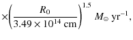
(Figs. 3a and 3d). We found
can be well described by power-law fits
(Figs. 3a and 3d). We found
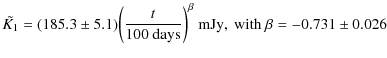
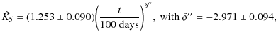
with reduced
We have neglected here the correlations between the various fitted parameters in the error determination, which is a good approximation given that the error in the magnetic field at day 100 mainly arises from the uncertainty in the source distance (9.4%) and the error in the power-law index b is dominated by the uncertainty in
The mean magnetic field given by Eq. (10) is in good agreement with the one obtained by Fransson & Björnsson (1998). But in contrast with the conclusions of these authors, the value of b obtained in the present analysis indicates that the scaling law
![]() can be excluded at the 90% confidence level. The discrepancy is partly due to the different assumptions made for the SN expansion. Indeed, Fransson & Björnsson (1998) assumed m=1 for t<100 days (i.e.
can be excluded at the 90% confidence level. The discrepancy is partly due to the different assumptions made for the SN expansion. Indeed, Fransson & Björnsson (1998) assumed m=1 for t<100 days (i.e.
![]() )
and m=0.74 at later epochs. The FFA model is also different in the two analyses. However, because the present result is restricted to relatively late epochs, it is only weakly dependent of the FFA modeling.
)
and m=0.74 at later epochs. The FFA model is also different in the two analyses. However, because the present result is restricted to relatively late epochs, it is only weakly dependent of the FFA modeling.
A ``pure'' SSA model calculated with
![]() and the best-fit power laws for
and the best-fit power laws for
![]() and
and
![]() (Eq. (9)) is shown in Fig. 2. We see that this model does not correctly represent the data taken before day 100. This is partly because free-free attenuation of the radio emission in the CSM was not taken into account. But it is also due to the strong radiative losses suffered by the radio-emitting electrons at early epochs (see Fransson & Björnsson 1998, and Sect. 3 below), which are not included in the parametric formalism of Weiler et al. (2002, and references therein) used here. As we will see below, one of the main effects of the electron energy losses is to reduce the flux density at short wavelengths during the transition from the optically thick to the optically thin regime. If this effect is not properly taken into account, the relative contributions of FFA and SSA at early epochs post-outburst cannot be reliably estimated. Consequently, the magnetic field determination for these epochs is uncertain. We assume here that the time evolution of
(Eq. (9)) is shown in Fig. 2. We see that this model does not correctly represent the data taken before day 100. This is partly because free-free attenuation of the radio emission in the CSM was not taken into account. But it is also due to the strong radiative losses suffered by the radio-emitting electrons at early epochs (see Fransson & Björnsson 1998, and Sect. 3 below), which are not included in the parametric formalism of Weiler et al. (2002, and references therein) used here. As we will see below, one of the main effects of the electron energy losses is to reduce the flux density at short wavelengths during the transition from the optically thick to the optically thin regime. If this effect is not properly taken into account, the relative contributions of FFA and SSA at early epochs post-outburst cannot be reliably estimated. Consequently, the magnetic field determination for these epochs is uncertain. We assume here that the time evolution of
![]() determined from day 75 after explosion was the same at earlier times.
determined from day 75 after explosion was the same at earlier times.
We also see in Fig. 2 that the decline with time of the optically-thin emission calculated in the SSA model is too slow as compared to the data at 20 cm. A possible explanation is that the energy distribution of the radiating electrons deviates from a power law of constant spectral index, as implicitly assumed in the above modeling (but see below).
The derived time dependence of
![]() is consistent with the scaling law originally adopted by Chevalier (1982b),
is consistent with the scaling law originally adopted by Chevalier (1982b),
![]() .
In Chevalier's model, the scaling law is based on the assumption that the postshock magnetic field is built up by a turbulent amplification powered by the total available postshock energy density. We will see in Sect. 4.3 that the temporal evolution
.
In Chevalier's model, the scaling law is based on the assumption that the postshock magnetic field is built up by a turbulent amplification powered by the total available postshock energy density. We will see in Sect. 4.3 that the temporal evolution
![]() is also to be expected if the magnetic field is amplified by Bell (2004)'s nonresonant cosmic-ray streaming instability in the shock precursor region and if furthermore the shock is not strongly modified by the back pressure from the energetic ions. We note that the time dependence
is also to be expected if the magnetic field is amplified by Bell (2004)'s nonresonant cosmic-ray streaming instability in the shock precursor region and if furthermore the shock is not strongly modified by the back pressure from the energetic ions. We note that the time dependence
![]() was also recently reported by Soderberg et al. (2008) for the type Ibc SN 2008D. Therefore, based on both observational evidences and a theoretical basis, I assume in the following that the postshock magnetic field results from an amplification by the cosmic-ray streaming instability operating in the shock precursor and that the field immediately upstream from the subshock is of the form
was also recently reported by Soderberg et al. (2008) for the type Ibc SN 2008D. Therefore, based on both observational evidences and a theoretical basis, I assume in the following that the postshock magnetic field results from an amplification by the cosmic-ray streaming instability operating in the shock precursor and that the field immediately upstream from the subshock is of the form
![]() ,
where Bu0 is a free parameter to be determined from fits to the radio data.
,
where Bu0 is a free parameter to be determined from fits to the radio data.
2.4 Nonlinear particle acceleration
![\begin{figure}
\par\includegraphics[width=15cm]{1511f4.eps}
\end{figure}](/articles/aa/full_html/2009/19/aa11511-08/img137.png) |
Figure 4:
Shocked proton and electron phase-space distributions vs. kinetic energy, at day 1000 after shock breakout. Following Berezhko & Ellison (1999), the phase-space distribution functions have been multiplied by
|
| Open with DEXTER | |
Particle acceleration at the forward shock is calculated with the semianalytic model of nonlinear DSA developed by Berezhko & Ellison (1999) and Ellison
et al. (2000). Although the model strictly applies to plane-parallel, steady state shocks, it has been successfully used by Ellison et al. (2000) for evolving SNRs and more recently by Tatischeff & Hernanz (2007) to describe the evolution of the blast wave generated in the 2006 outburst of the recurrent nova RS Ophiuchi. The main feature of this relatively simple model is to approximate the nonthermal part of the shocked proton and electron phase-space distributions as a three-component power law with an exponential cutoff at high momenta,
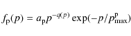
and
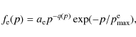
where the power-law index q(p), which is the same for protons and electrons, can have three different decreasing values in the momentum ranges
The maximum proton momentum
![]() is calculated either by time integration of the DSA rate (i.e., shock age limitation) or by equalling the upstream diffusion length to some fraction
is calculated either by time integration of the DSA rate (i.e., shock age limitation) or by equalling the upstream diffusion length to some fraction
![]() of the shock radius (i.e., particle escape limitation), whichever produces the lowest value of
of the shock radius (i.e., particle escape limitation), whichever produces the lowest value of
![]() (see, e.g., Baring et al. 1999). Following, e.g., Ellison & Cassam-Chenaï (2005), I take
(see, e.g., Baring et al. 1999). Following, e.g., Ellison & Cassam-Chenaï (2005), I take
![]() .
To estimate the spatial diffusion coefficient,
.
To estimate the spatial diffusion coefficient,
![]() ,
the scattering mean free path
,
the scattering mean free path ![]() of all particles of speed v is assumed to be
of all particles of speed v is assumed to be
![]() (Ellison et al. 2000), where
(Ellison et al. 2000), where ![]() is the particle gyroradius and
is the particle gyroradius and
![]() is a constant that characterizes the scattering strength. I use
is a constant that characterizes the scattering strength. I use
![]() ,
which is a typical value for young SNRs (Parizot et al. 2006). The maximum electron momentum
,
which is a typical value for young SNRs (Parizot et al. 2006). The maximum electron momentum
![]() is limited by synchrotron and inverse Compton losses (see Sect. 2.6).
is limited by synchrotron and inverse Compton losses (see Sect. 2.6).
Given the upstream sonic and Alfvén Mach numbers of the shock, which can be readily calculated from ![]() ,
,
![]() ,
,
![]() ,
and Bu0 (see below), the proton distribution function (i.e. the normalization
,
and Bu0 (see below), the proton distribution function (i.e. the normalization ![]() and power-law
index q(p)) is determined by an arbitrary injection parameter
and power-law
index q(p)) is determined by an arbitrary injection parameter
![]() ,
which is the fraction of total shocked protons in protons with momentum
,
which is the fraction of total shocked protons in protons with momentum
![]() injected from the postshock thermal pool into the DSA process. The work of Blasi et al. (2005) allows us to accurately relate the proton injection momentum
injected from the postshock thermal pool into the DSA process. The work of Blasi et al. (2005) allows us to accurately relate the proton injection momentum
![]() to
to
![]() .
.
The normalization of the electron distribution function is obtained from (Ellison et al. 2000)
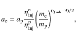
where

where
Alfvén wave heating of the shock precursor is taken into account from the simple formalism given in Berezhko & Ellison (1999). However, a small change to the model of these authors is adopted here: the Alfvén waves are assumed to propagate isotropically in the precursor region and not only in the direction opposite to the plasma flow, i.e. Eqs. (52) and (53) of Berezhko & Ellison (1999) are not used. This is a reasonable assumption (see, e.g., Bell & Lucek 2001) given the strong, nonlinear magnetic field amplification required to explain the radio emission from SN 1993J.
Figure 4 shows calculated shocked proton and electron phase-space distributions for three sets of injection parameters (
![]() ,
,
![]() )
that will be used in Sect. 3.2 to model the radio light curves. The thermal Maxwell-Boltzmann components were calculated using the shocked proton temperature
)
that will be used in Sect. 3.2 to model the radio light curves. The thermal Maxwell-Boltzmann components were calculated using the shocked proton temperature
![]() determined by the nonlinear DSA model (see, e.g., Ellison et al. 2000) and arbitrarily assuming the temperature ratio
determined by the nonlinear DSA model (see, e.g., Ellison et al. 2000) and arbitrarily assuming the temperature ratio
![]() .
Noteworthy, the nonthermal electron distribution is independent of
.
Noteworthy, the nonthermal electron distribution is independent of
![]() when
when
![]() is specified (see Eq. (13)) except for the electron injection momentum
is specified (see Eq. (13)) except for the electron injection momentum
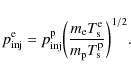
The uncertain temperature ratio has thus practically no influence on the modeled radio emission.
We see in Fig. 4a that for
![]() the well-known test-particle result q(p)=4 is recovered. But for
the well-known test-particle result q(p)=4 is recovered. But for
![]() (Figs. 4b and c) the nonlinear shock modification becomes significant. In particular we see that the nonthermal electron distribution steepens below
(Figs. 4b and c) the nonlinear shock modification becomes significant. In particular we see that the nonthermal electron distribution steepens below ![]() GeV with increasing
GeV with increasing
![]() ,
as a result of the decrease of
,
as a result of the decrease of
![]() (Eq. (14)). This is important because the radio emission from SN 1993J is produced by relativistic electrons of energies <1 GeV.
(Eq. (14)). This is important because the radio emission from SN 1993J is produced by relativistic electrons of energies <1 GeV.
Figure 5 shows calculated subshock and total compression ratios for the case
![]() which, as will be shown in Sect. 3.2, provides the best description of the radio light curves. The calculations were performed with the upstream sonic Mach number
which, as will be shown in Sect. 3.2, provides the best description of the radio light curves. The calculations were performed with the upstream sonic Mach number
![]() ,
given the upstream sound velocity
,
given the upstream sound velocity
![]() km s-1 for
km s-1 for
![]() K. Here
K. Here
![]() is the adiabatic index for an ideal non-relativistic gas, k is the Boltzmann's constant, and
is the adiabatic index for an ideal non-relativistic gas, k is the Boltzmann's constant, and
![]() .
Given the magnetic field immediately upstream from the subshock
.
Given the magnetic field immediately upstream from the subshock
![]() ,
the Alfvén Mach number
,
the Alfvén Mach number
![]() is independent of time; here
is independent of time; here
![]() is the Alfvén velocity. Anticipating the results presented in Sect. 3, with the best-fit parameter values Bu0=50 G and
is the Alfvén velocity. Anticipating the results presented in Sect. 3, with the best-fit parameter values Bu0=50 G and
![]() yr-1, we have
yr-1, we have
![]() .
Thus,
.
Thus,
![]() ,
which implies that energy should be very efficiently transfered from the accelerated particles to the thermal gas via Alfvén wave dissipation in the shock precursor region (Berezhko & Ellison 1999). The resulting increase in the gas pressure ahead of the viscous subshock limits the overall compression ratio,
,
which implies that energy should be very efficiently transfered from the accelerated particles to the thermal gas via Alfvén wave dissipation in the shock precursor region (Berezhko & Ellison 1999). The resulting increase in the gas pressure ahead of the viscous subshock limits the overall compression ratio,
![]() ,
to values close to 4 (i.e. the standard value for a test-particle strong shock).
,
to values close to 4 (i.e. the standard value for a test-particle strong shock).
![\begin{figure}
\par\includegraphics[width=8.8cm]{1511f5.eps}
\end{figure}](/articles/aa/full_html/2009/19/aa11511-08/img181.png) |
Figure 5:
Subshock and total compression ratios at the forward shock ( left axis) and nonthermal energy fraction
|
| Open with DEXTER | |
However, we see in Fig. 5 that the acceleration efficiency
![]() increases with time. This quantity is defined as the fraction of total incoming energy flux,
increases with time. This quantity is defined as the fraction of total incoming energy flux,
![]() ,
going into shock-accelerated nonthermal particles. At day 3100 after outburst, when the shock has reached the outer boundary of the dense progenitor wind,
,
going into shock-accelerated nonthermal particles. At day 3100 after outburst, when the shock has reached the outer boundary of the dense progenitor wind,
![]() %. The subshock compression ratio is found to slowly decrease with time, as the shock becomes increasingly modified. Thus, we expect a gradual steepening with time of the electron distribution between
%. The subshock compression ratio is found to slowly decrease with time, as the shock becomes increasingly modified. Thus, we expect a gradual steepening with time of the electron distribution between
![]() and
and
![]() (Eq. (14)).
(Eq. (14)).
Given the high turbulent magnetic field in the shock region, the timescale for diffusive acceleration of electrons in this momentum range is very rapid,
![]() h. This is much shorter than the characteristic timescale for variation of the shock structure (see Fig. 5), so it is justified to assume that the spectrum of the radio-emitting electrons at a given time is determined by the instantaneous subshock compression ratio at that time. We note, however, that
our calculation of the high-energy end of the proton spectrum is not accurate, because the acceleration timescale for the highest energy particles is much longer.
h. This is much shorter than the characteristic timescale for variation of the shock structure (see Fig. 5), so it is justified to assume that the spectrum of the radio-emitting electrons at a given time is determined by the instantaneous subshock compression ratio at that time. We note, however, that
our calculation of the high-energy end of the proton spectrum is not accurate, because the acceleration timescale for the highest energy particles is much longer.
2.5 Magnetohydrodynamic evolution of the postshock plasma
![\begin{figure}
\par\includegraphics[width=8.8cm]{1511f6.eps}
\end{figure}](/articles/aa/full_html/2009/19/aa11511-08/img187.png) |
Figure 6:
Radial profiles of a) the gas density and b) the total magnetic field in the shock region. The density is normalized to the upstream value
|
| Open with DEXTER | |
The hydrodynamic evolution of the postshock plasma is calculated using the self-similar model (Chevalier 1982a,1983; Nadyozhin 1985) with the deceleration parameter m=0.83 (Sect. 2.1), the standard s=2 density profile (Sect. 2.2), and the adiabatic index
![]() .
Thus, the effects of the back pressure from the accelerated ions on the dynamics of the SNR are neglected. It is a good approximation for SN 1993J given that
.
Thus, the effects of the back pressure from the accelerated ions on the dynamics of the SNR are neglected. It is a good approximation for SN 1993J given that
![]() for the best parameter value
for the best parameter value
![]() (Fig. 5). The situation is different in older SNRs, such as the remnant of Kepler's (Decourchelle et al. 2000) and Tycho's (Warren et al. 2005) SNe. In these objects, the backreaction of shock-accelerated cosmic rays has more influence on the shock structure, mainly because the magnetic field in the precursor region is much lower than for SN 1993J, such that Alfvén wave heating is less important.
(Fig. 5). The situation is different in older SNRs, such as the remnant of Kepler's (Decourchelle et al. 2000) and Tycho's (Warren et al. 2005) SNe. In these objects, the backreaction of shock-accelerated cosmic rays has more influence on the shock structure, mainly because the magnetic field in the precursor region is much lower than for SN 1993J, such that Alfvén wave heating is less important.
Figure 6a shows the density profile in the region of interaction between the SN ejecta and the progenitor wind. The locations of the forward and reverse shocks are clearly visible, at 1.27 and 0.976 times the radius of the contact discontinuity, respectively.
The postshock magnetic field is thought to result from the shock compression of the turbulent magnetic field immediately upstream from the subshock, that has been presumably amplified in the precursor region by both resonant (Bell & Lucek 2001) and nonresonant (Bell 2004) cosmic-ray streaming instabilities. Following the work of Cassam-Chenaï et al. (2007) for Tycho's SNR, I make two different assumptions about the postshock magnetic field evolution: one where the turbulent magnetic field is simply carried by the downstream plasma flow (i.e. advected) and another where the magnetic turbulence is rapidly damped behind the blast wave.
2.5.1 Advected downstream magnetic field
The equations describing the evolution of the postshock magnetic field in the case of pure advection in the downstream plasma are given in Cassam-Chenaï
et al. (2005) and references therein. They are reproduced here for sake of convenience. Let the radial and tangential components of the immediate postshock magnetic field be Bd,r and Bd,t, respectively. Assuming that the upstream magnetic field is fully turbulent and isotropic, we have
At time t after outburst, the radial and tangential components of the magnetic field in a fluid element with density
where ti is the earlier time when this fluid element was shocked and

The radial profile of the total advected magnetic field is shown in Fig. 6b. Under the assumption of self-similarity, the plotted ratio B(R)/Bd is independent of time.
2.5.2 Damped downstream magnetic field
Pohl et al. (2005) suggested that the nonthermal X-ray filaments observed in Galactic SNRs could be localized enhancements of the magnetic field in the blast wave region. In this scenario, the turbulent magnetic field amplified in the shock presursor is thought to be rapidly damped behind the shock front by cascading of wave energy to very small scales where it is ultimately dissipated.
Assuming a Kolmogorov-type energy cascade of incompressible magnetohydrodynamic (MHD) turbulence, the characteristic damping length can be estimated to be (Pohl
et al. 2005; see also Cassam-Chenaï et al. 2007)
where
such that
For
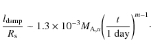
We see that for
Pohl et al. (2005) also considered that downstream magnetic field damping can result from cascading of fast-mode and Alvén waves in background
MHD turbulence. In these cases, we have (see also Cassam-Chenaï et al. 2007)
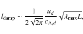
where L is the outer scale of the pre-existing MHD turbulence. Assuming that this quantity is of the order of the diameter of the dense wind bubble blown by the red supergiant progenitor of the SN,
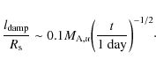
This damping length is thus always larger (for t<3100 days) than the one estimated from the general model of Kolmogorov-type energy cascade (Eq. (24)). In the case of damping by cascading of fast-mode and Alfvén waves the spatial relaxation of the postshock magnetic field follows an exponential decay law
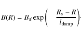
Postshock magnetic field profiles obtained from Eqs. (26) and (27) with
2.6 Nonthermal electron energy losses
The cooling processes that can affect the energy distribution of the nonthermal electrons during the SN expansion were studied by Fransson & Björnsson (1998). They found synchrotron cooling to be predominant for electrons radiating at short wavelengths for most of the time, Coulomb cooling to be potentially important at early epochs post-outburst, adiabatic cooling to be dominant for electrons radiating at 20 cm at late epochs and inverse Compton losses due to electron scattering off photons from the SN photosphere to be less important. These results depend, however, on several model parameters, e.g. the progenitor mass loss rate
![]() and the magnetic field Bu0.
and the magnetic field Bu0.
With the best parameter values of the present model, Coulomb cooling is found to be more important than synchrotron cooling only at very early epochs, when the radio emission is still optically thick to SSA (Sect. 4.2). At that time, the energy losses of the shock-accelerated electrons have little if no effect on the radio emission, such that Coulomb cooling can be safely neglected. This contrasts with the model of Fransson & Björnsson (1998).
I use the work of Reynolds (1998; see also Cassam-Chenaï et al. 2007, Appendix B) to calculate the downstream evolution of the electron energy distribution due to synchrotron, inverse Compton, and adiabatic losses. The number density of nonthermal electrons per unit energy interval at kinetic energy E in a fluid element being at the downstream position R at time t can be written as
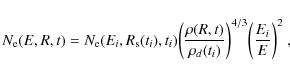
where
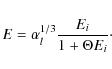
Here,
![\begin{displaymath}\Theta = {4 \over 3} {\sigma_{\rm T} c \over (m_{\rm e}c^2)^2...
...} + U_{\rm rad}(\tau) \bigg] \alpha_l^{1/3}(\tau) {\rm d}\tau,
\end{displaymath}](/articles/aa/full_html/2009/19/aa11511-08/img215.png)
where
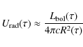
is the energy density in the radiation field,
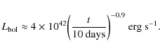
Fransson & Björnsson (1998) showed that during the first ![]() 100 days after outburst, the radiation energy density at the forward shock position was dominated by emission from the SN ejecta. They approximated the bolometric luminosity of SN 1993J at these early epochs by
100 days after outburst, the radiation energy density at the forward shock position was dominated by emission from the SN ejecta. They approximated the bolometric luminosity of SN 1993J at these early epochs by
The ratio of the energy densities of magnetic to seed photon fields in the immediate postshock region is then
This result shows that Compton cooling can play a role soon after outburst depending on the magnetic field strength, but that synchrotron cooling is expected to become more important after some time. A similar result was found by Chevalier & Fransson (2006) for type Ib/c SNe.
2.7 Radio synchrotron emission
Once the electron energy distribution and the magnetic field as a function of downstream position are determined as explained above, the synchrotron brightness profile and the total flux density at a given time can be calculated as described in Appendix B.
3 Results
For a given assumption about the evolution of the postshock magnetic turbulence (advection or damping), the model has four main parameters to be fitted to the radio data: the mass loss rate of the red supergiant progenitor,
![]() ,
the normalization of the upstream magnetic field, Bu0, and the proton and electron injection parameters,
,
the normalization of the upstream magnetic field, Bu0, and the proton and electron injection parameters,
![]() and
and
![]() .
In addition, the radius of the absorbing disk,
.
In addition, the radius of the absorbing disk,
![]() ,
that accounts for FFA of the radio emission by the inner SN ejecta (see Appendix B) mainly influences the brightness profile as a function of angular radius. We first compare calculated synchrotron profiles with the high-resolution profile at 3.6 cm measured by Bietenholz et al. (2003) from VLBI observations. We then study the radio light curves reported by Weiler et al. (2007).
,
that accounts for FFA of the radio emission by the inner SN ejecta (see Appendix B) mainly influences the brightness profile as a function of angular radius. We first compare calculated synchrotron profiles with the high-resolution profile at 3.6 cm measured by Bietenholz et al. (2003) from VLBI observations. We then study the radio light curves reported by Weiler et al. (2007).
3.1 The radial brightness profile
To study the radial brightness profile of SN 1993J with the highest angular resolution, Bietenholz et al. (2003) produced a composite image at 8.4 GHz from VLBI observations performed at t=2080, 2525, and 2787 days after explosion. The data were appropriately scaled to take into account the SN expansion and then averaged. The resulting brightness profile versus angular radius is shown in Fig. 7 together with two calculated profiles. Here and in the following, we set the radius of the inner opaque disk accounting for FFA of the radio emission from the side of the shell moving away from us (Appendix B) to
![]() .
We see in Fig. 7 that this simple model of absorption by the SN ejecta is consistent with the data for
.
We see in Fig. 7 that this simple model of absorption by the SN ejecta is consistent with the data for
![]() ,
but underestimates the observed emission for
,
but underestimates the observed emission for
![]() .
The difference might arise from incomplete absorption of the radio waves in the inner ejecta, possibly because the latter are filamentary (see Bietenholz et al. 2003). However, the excess of emission at
.
The difference might arise from incomplete absorption of the radio waves in the inner ejecta, possibly because the latter are filamentary (see Bietenholz et al. 2003). However, the excess of emission at
![]() accounts for only
accounts for only ![]() 3% of the total flux density and it has been neglected so as to limit the number of free parameters.
3% of the total flux density and it has been neglected so as to limit the number of free parameters.
![\begin{figure}
\par\includegraphics[width=8.8cm]{1511f7.eps}
\end{figure}](/articles/aa/full_html/2009/19/aa11511-08/img226.png) |
Figure 7:
Relative brightness of the 3.6 cm emission from SN 1993J at day 2787 after outburst, as a function of angular radius. In the calculations, the outer angular radius |
| Open with DEXTER | |
![\begin{figure}
\par\includegraphics[width=8.8cm]{1511f8.eps}
\end{figure}](/articles/aa/full_html/2009/19/aa11511-08/img228.png) |
Figure 8:
Calculated radial profiles of the relative emissivity at 3.6 cm and
|
| Open with DEXTER | |
The radial brightness profile is mainly sensitive to the strength and profile of the magnetic field behind the blast wave![]() . The two calculated profiles shown in Fig. 7 are for Bu0=50 G and the case of pure advection of the field in the downstream plasma. We see in Fig. 7b that the model with only electrons accelerated at the forward shock (red dashed curve) produces a peak at
. The two calculated profiles shown in Fig. 7 are for Bu0=50 G and the case of pure advection of the field in the downstream plasma. We see in Fig. 7b that the model with only electrons accelerated at the forward shock (red dashed curve) produces a peak at
![]() that is both slightly shifted and too narrow as compared to the observed one. There is clearly a deficit of emission at
that is both slightly shifted and too narrow as compared to the observed one. There is clearly a deficit of emission at
![]() ,
i.e. from a region close to the contact discontinuity that marks the border between shocked ejecta and shocked CSM (see Fig. 6).
,
i.e. from a region close to the contact discontinuity that marks the border between shocked ejecta and shocked CSM (see Fig. 6).
As shown in Fig. 8, the radial emissivity of electrons accelerated at the blast wave is cut off before it reaches the contact discontinuity. This is due to the strong radiative losses suffered by the electrons that have been accelerated at the earliest epochs. The cutoff exists whatever the magnetic fied strength Bu0; it is mainly produced by Compton cooling for
![]() G (see Eq. (33)). Thus, the missing component of synchrotron emission is probably coming from another source of accelerated electrons, most likely the reverse shock. The efficiency of particle acceleration at reverse shocks in SNRs is poorly known, because it depends on the unknown amplification of the magnetic field in the unshocked ejecta material (Ellison et al. 2005). However, recent observations of SNRs provide clear evidence for synchrotron emission associated with reverse shocks (see Helder & Vink 2008 for Cassiopeia A). Here, we simply model this emission by a shell of uniform emissivity between the reverse shock and the contact discontinuity (Fig. 8), whose normalization is fitted to the radial brightness profile measured by Bietenholz et al. (2003). We use as normalization factor the integral of the radial emissivity relative to that for the forward shock:
G (see Eq. (33)). Thus, the missing component of synchrotron emission is probably coming from another source of accelerated electrons, most likely the reverse shock. The efficiency of particle acceleration at reverse shocks in SNRs is poorly known, because it depends on the unknown amplification of the magnetic field in the unshocked ejecta material (Ellison et al. 2005). However, recent observations of SNRs provide clear evidence for synchrotron emission associated with reverse shocks (see Helder & Vink 2008 for Cassiopeia A). Here, we simply model this emission by a shell of uniform emissivity between the reverse shock and the contact discontinuity (Fig. 8), whose normalization is fitted to the radial brightness profile measured by Bietenholz et al. (2003). We use as normalization factor the integral of the radial emissivity relative to that for the forward shock:
where
![\begin{figure}
\par\includegraphics[width=8.8cm]{1511f9.eps}
\end{figure}](/articles/aa/full_html/2009/19/aa11511-08/img236.png) |
Figure 9:
Same as Fig. 7 but for Bu0=30 G,
|
| Open with DEXTER | |
Figure 8 also shows that the radial emissivity profile decreases more rapidly behind the blast wave as Bu0 increases, which is due to the synchrotron energy losses. Brightness profiles calculated for Bu0=30 and 80 G are compared to the data in Fig. 9. We adjusted the value of
![]() so as to match the maximum of the relative brightness to the observed one at
so as to match the maximum of the relative brightness to the observed one at
![]() .
But we see that the width of the broad emission peak is not well fitted: the calculated emission profile is too narrow (resp. too broad) for the low (resp. high) value of Bu0. Thus, the high-resolution brightness profile of Bietenholz et al. provides a first indication of the magnetic field strength in the blast wave region: 11<Bu<29 mG at day 2787 post-outburst (
30<Bu0<80 G).
.
But we see that the width of the broad emission peak is not well fitted: the calculated emission profile is too narrow (resp. too broad) for the low (resp. high) value of Bu0. Thus, the high-resolution brightness profile of Bietenholz et al. provides a first indication of the magnetic field strength in the blast wave region: 11<Bu<29 mG at day 2787 post-outburst (
30<Bu0<80 G).
The measured profile also constraints the evolution of the postshock magnetic field. Figure 10 shows that, when the magnetic field is damped behind the blast wave, the brightness angular distribution is shifted toward the outer edge of the radio shell and the resulting profile is clearly not consistent with the data. This conclusion is independent of both the value of Bu and the reverse shock contribution. In particular, the brightness profile becomes clearly too broad when
![]() is increased so as to set the maximum of the emission at
is increased so as to set the maximum of the emission at
![]() .
.
The contact interface between the SN ejecta and the shocked CSM is thought to be Rayleigh-Taylor unstable and it has been suggested that the associated turbulence can amplify the postshock magnetic field (Chevalier et al. 1992; Jun & Norman 1996). This would increase the synchrotron losses near the contact discontinuity. Consequently, the position of the cutoff in the radial emissivity would likely be shifted to larger radii with respect to the case with no amplification of the postshock magnetic field (Fig. 8). As a result, a larger contribution of synchrotron radiation from electrons accelerated at the reverse shock would probably be needed to reproduce the measured brightness profile.
However, the shocked CSM is expected to be strongly magnetized due to the field amplification by the cosmic-ray streaming instability operating in the forward shock precursor and the postshock magnetic field profile is expected to be dominated by the tangential component (see Eqs. (18) and (19)). Such a strong magnetic field could decrease the growth of the Rayleigh-Taylor instability and limit a possible additional amplification of the field by the turbulence associated with this instability (Jun et al. 1995). This aspect of the magnetohydrodynamic evolution of the postshock plasma certainly deserves further studies. Here, we assume that the postshock magnetic field is not significantly amplified by the Rayleigh-Taylor instability.
![\begin{figure}
\par\includegraphics[width=8.8cm]{1511f10.eps}
\end{figure}](/articles/aa/full_html/2009/19/aa11511-08/img239.png) |
Figure 10:
Same as Fig. 7 but for the damping of the magnetic turbulence downstream ( green dashed lines) compared to the advection of the shocked plasma ( blue solid lines). In both cases, Bu0=50 G and
|
| Open with DEXTER | |
![\begin{figure}
\par\includegraphics[width=13cm]{1511f11.eps}
\end{figure}](/articles/aa/full_html/2009/19/aa11511-08/img240.png) |
Figure 11:
Radio light curves for SN 1993J at 0.3, 1.2, 2, 3.6, 6, and 20 cm. The data are from Weiler et al. (2007) and references therein. The blue solid lines represent the best-fit model, which is obtained for
|
| Open with DEXTER | |
3.2 Radio light curves
In the modeling of the radio light curves, we take into account the emission from electrons accelerated at the reverse shock assuming
![]() % at all times. As discussed above, this emission is then estimated to contribute to a maximum
of 17% of the total flux density. This number is an upper limit, because the synchrotron radiation from the inner shock is strongly attenuated when the emission associated with the forward shock is optically thick to SSA. We also assume
% at all times. As discussed above, this emission is then estimated to contribute to a maximum
of 17% of the total flux density. This number is an upper limit, because the synchrotron radiation from the inner shock is strongly attenuated when the emission associated with the forward shock is optically thick to SSA. We also assume
![]() at all epochs. The resulting uncertainty on the flux density is negligible.
at all epochs. The resulting uncertainty on the flux density is negligible.
![\begin{figure}
\par\includegraphics[width=12cm]{1511f12.eps}
\end{figure}](/articles/aa/full_html/2009/19/aa11511-08/img241.png) |
Figure 12:
Radio light curves of SN 1993J with the flux density multiplied by
|
| Open with DEXTER | |
![\begin{figure}
\par\includegraphics[width=12cm]{1511f13.eps}
\end{figure}](/articles/aa/full_html/2009/19/aa11511-08/img242.png) |
Figure 13:
Same as Fig. 12 but for various values of the injection parameters:
|
| Open with DEXTER | |
Light curves calculated with the best-fit model are shown in Fig. 11. They were obtained for
![]() yr-1, Bu0=50 G,
yr-1, Bu0=50 G,
![]() ,
,
![]() ,
and pure advection of the postshock magnetic field. We see that the general features of the data are fairly well represented. But the associated reduced
,
and pure advection of the postshock magnetic field. We see that the general features of the data are fairly well represented. But the associated reduced ![]() is
is
![]() (
(
![]() for 554 degrees of freedom), which is comparable to the one of the best-fit semi-empirical model of Weiler et al. (2007):
for 554 degrees of freedom), which is comparable to the one of the best-fit semi-empirical model of Weiler et al. (2007):
![]()
![]() . However, in the comparison of the
. However, in the comparison of the ![]() values, one could note that the formalism of Weiler et al. has nine free parameters (Appendix A), against only four in the present model. Interestingly, the present model is also good at representing the 12 data points at 0.3 cm (
values, one could note that the formalism of Weiler et al. has nine free parameters (Appendix A), against only four in the present model. Interestingly, the present model is also good at representing the 12 data points at 0.3 cm (
![]() ), which is not the case for the parametric model of Weiler
et al. (
), which is not the case for the parametric model of Weiler
et al. (
![]() ;
see Fig. 2). The 0.3 cm flux density between
;
see Fig. 2). The 0.3 cm flux density between ![]() 10 and
10 and ![]() 40 days after outburst is lower in the present calculations than in previous ones, because the strong synchrotron losses suffered by the radiating electrons during the early SN expansion are now taken into account. The difference is more pronounced at the shortest wavelength, because this emission is produced by higher-energy electrons (on average), for which the synchrotron cooling time is lower (
40 days after outburst is lower in the present calculations than in previous ones, because the strong synchrotron losses suffered by the radiating electrons during the early SN expansion are now taken into account. The difference is more pronounced at the shortest wavelength, because this emission is produced by higher-energy electrons (on average), for which the synchrotron cooling time is lower (
![]() ,
,
![]() being the electron Lorentz factor; see Sect. 4.2). Obviously, this effect cannot be accounted for by models neglecting the electron energy losses and assuming a homogeneous shell of emission (Chevalier 1982b,1998;
Pérez-Torres et al. 2001; Weiler et al. 2002; Soderberg et al. 2005).
being the electron Lorentz factor; see Sect. 4.2). Obviously, this effect cannot be accounted for by models neglecting the electron energy losses and assuming a homogeneous shell of emission (Chevalier 1982b,1998;
Pérez-Torres et al. 2001; Weiler et al. 2002; Soderberg et al. 2005).
However, significant deviations of the best-fit model from the data can be observed in Fig. 11. In particular, we see that the straight rising branches of the calculated light curves do not represent well the observations at 2 and 3.6 cm. This is most likely due to our treatment of external FFA (Sect. 2.2). It is possible that the structure of the CSM was more complicated at the time of explosion than that implicitly assumed by adopting an attenuation of the form
![]() with
with
![]() .
This would be the case if, for example, the filling factor of clumpy material was not constant throughout the whole CSM. It is also possible that the CSM temperature
.
This would be the case if, for example, the filling factor of clumpy material was not constant throughout the whole CSM. It is also possible that the CSM temperature
![]() was not uniform but varied with radius. However, we note that the data at 6 and 20 cm are very well fitted. The best-fit normalization to the FFA optical depth is
was not uniform but varied with radius. However, we note that the data at 6 and 20 cm are very well fitted. The best-fit normalization to the FFA optical depth is
![]() ,
which gives from Eq. (8)
,
which gives from Eq. (8)
![]() yr-1.
yr-1.
Like for the brightness profile, the light curves provide clear evidence that the postshock magnetic field is essentially advected behind the shock. Indeed, we see in Fig. 11 that the synchrotron flux declines much too rapidly after about day 100 in the model with damping of magnetic turbulence.
The modeling of external FFA being uncertain, we now focus on the optically thin parts of the radio emission. In Figs. 12 and 13, the flux density is multiplied by a time-dependent power law to set upright the decreasing parts of the light curves and the vertical scale is expanded. Figure 12 shows the effect of changing the magnetic field strength. For each value of Bu0, the electron injection rate was adjusted to provide a decent fit to the data at 3.6 cm. We see that only the model with Bu0=50 G represents the data at all the other wavelengths reasonably well. For example, for
Bu0=100 G the calculated flux densities at 0.3 cm fall short of the data, whereas those at 20 cm are too high in the optically thin phase. This effect is due to the process of synchrotron cooling, whose rate increases with the magnetic field (
![]() )
and which steepens the energy distribution of the accelerated electrons during their advection downstream. Thus, the mean propagated spectrum of nonthermal electrons is too steep (resp. too hard) for
Bu0=100 G (resp. Bu0=20 G) to provide a good fit to the data at all frequencies. It is remarkable that when the synchrotron losses are taken into account, the degeneracy for the optically-thin emission between the magnetic field and the nonthermal electron density (e.g. Chevalier 1998) is lifted.
)
and which steepens the energy distribution of the accelerated electrons during their advection downstream. Thus, the mean propagated spectrum of nonthermal electrons is too steep (resp. too hard) for
Bu0=100 G (resp. Bu0=20 G) to provide a good fit to the data at all frequencies. It is remarkable that when the synchrotron losses are taken into account, the degeneracy for the optically-thin emission between the magnetic field and the nonthermal electron density (e.g. Chevalier 1998) is lifted.
Figure 13 shows the effect of changing
![]() .
The values of the electron injection parameter are somewhat arbitrary, except for the case
.
The values of the electron injection parameter are somewhat arbitrary, except for the case
![]() .
We see that in the test-particle case (
.
We see that in the test-particle case (
![]() ), the decline of the optically-thin emission with time is too slow as compared to the data. This provides evidence that the pressure from accelerated ions is important to the structure of the blast wave. But we also see that for
), the decline of the optically-thin emission with time is too slow as compared to the data. This provides evidence that the pressure from accelerated ions is important to the structure of the blast wave. But we also see that for
![]() the light curves decline too rapidly, which shows that the shock modification is relatively weak. There is a partial correlation between
the light curves decline too rapidly, which shows that the shock modification is relatively weak. There is a partial correlation between
![]() and Bu0. By varying these two parameters and comparing the calculated curves to the data, I estimate the acceptable range for the proton injection rate to be
and Bu0. By varying these two parameters and comparing the calculated curves to the data, I estimate the acceptable range for the proton injection rate to be
![]() .
Higher values of
.
Higher values of
![]() are often used in studies of Galactic SNRs
(e.g., Cassam-Chenaï et al. 2007, adopted
are often used in studies of Galactic SNRs
(e.g., Cassam-Chenaï et al. 2007, adopted
![]() for Tycho's remnant, based on the observed closeness of the blast wave and contact discontinuity).
for Tycho's remnant, based on the observed closeness of the blast wave and contact discontinuity).
The time evolution of the synchrotron flux is related to the energy distribution of the emitting electrons (see, e.g., Chevalier 1982b): the steeper the electron spectrum, the faster the decline of the optically-thin emission. As dicussed in Sect. 2.4, the main effect of the cosmic-ray pressure is to reduce the compression ratio of the subshock,
![]() ,
whereas the overall compression ratio
,
whereas the overall compression ratio
![]() remains nearly constant. This shock modification affects essentially the particles of energies
remains nearly constant. This shock modification affects essentially the particles of energies
![]() that remain in the vicinity of the subshock during the DSA process. As shown in Fig. 4, an increase of
that remain in the vicinity of the subshock during the DSA process. As shown in Fig. 4, an increase of
![]() causes the energy distribution of the nonthermal electrons to steepens below
causes the energy distribution of the nonthermal electrons to steepens below ![]() 1 GeV, which is the relevant energy domain for the radio synchrotron emission. The light curves provide evidence that the spectral index of the shocked electrons in this energy range is slightly higher than the test-particle value
1 GeV, which is the relevant energy domain for the radio synchrotron emission. The light curves provide evidence that the spectral index of the shocked electrons in this energy range is slightly higher than the test-particle value
![]() ,
which is effectively obtained with
,
which is effectively obtained with
![]() .
.
![\begin{figure}
\par\includegraphics[width=12cm]{1511f14.eps}
\end{figure}](/articles/aa/full_html/2009/19/aa11511-08/img258.png) |
Figure 14:
Same as Fig. 11 but for a CSM density profile of the form
|
| Open with DEXTER | |
Although in most previous models of radio emission from SNe the shocked-electron spectral index is assumed to remain constant, a gradual steepening with time of the shocked-particle energy spectrum below
![]() is to be expected. This is because of the decrease of the upstream magnetic field, which reduces the efficiency of gas heating via Alfvén wave damping in the precursor region and consequently reduces the subshock compression ratio. Thus, for
is to be expected. This is because of the decrease of the upstream magnetic field, which reduces the efficiency of gas heating via Alfvén wave damping in the precursor region and consequently reduces the subshock compression ratio. Thus, for
![]() ,
we find that
,
we find that
![]() decreases from 3.89 to 3.70 between day 10 and day 3100 after outburst (Fig. 5), which causes
decreases from 3.89 to 3.70 between day 10 and day 3100 after outburst (Fig. 5), which causes
![]() to increase from 4.04 to 4.11 (Eq. (14)).
to increase from 4.04 to 4.11 (Eq. (14)).
For given values of Bu0 and
![]() ,
the normalization of the optically-thin synchrotron flux is set by the product
,
the normalization of the optically-thin synchrotron flux is set by the product
![]() .
As the progenitor mass loss rate also fixes the level of FFA in the CSM, the electron injection rate can be uniquely determined. For
.
As the progenitor mass loss rate also fixes the level of FFA in the CSM, the electron injection rate can be uniquely determined. For
![]() ,
the best-fit parameter is
,
the best-fit parameter is
![]() .
To set the amplitude of the nonthermal electron spectrum in DSA models, several authors use the electron-to-proton density ratio at relativistic energies,
.
To set the amplitude of the nonthermal electron spectrum in DSA models, several authors use the electron-to-proton density ratio at relativistic energies,
![]() ,
rather than the electron injection rate (e.g., Ellison et al. 2000). Here, we obtain at, e.g., 10 GeV
,
rather than the electron injection rate (e.g., Ellison et al. 2000). Here, we obtain at, e.g., 10 GeV
![]() at day 10 and
at day 10 and
![]() at day 3100. The value of
at day 3100. The value of
![]() is higher at day 10 because
is higher at day 10 because
![]() is lower (see Eq. (13)). The obtained values of
is lower (see Eq. (13)). The obtained values of
![]() are roughly consistent with those estimated for the blast wave of Tycho's SNR:
are roughly consistent with those estimated for the blast wave of Tycho's SNR:
![]() (Völk
et al. 2002),
(Völk
et al. 2002),
![]() 1-
1-
![]() (Cassam-Chenaï et al. 2007).
(Cassam-Chenaï et al. 2007).
4 Discussion
The model gives a consistent description of the large set of radio data available for SN 1993J. In particular, it is remarkable that the same magnetic field strength,
![]() G (in
G (in
![]() ), is required to explain the high-resolution brightness profile measured by Bietenholz et al. (2003) at day 2787 after outburst and the set of radio light curves reported by Weiler et al. (2007). This further supports the assumption that the magnetic field at the shock varies approximately as 1/t. Besides, both the brightness profile and the light curves show that the postshock magnetic field is not damped behind the blast wave but simply carried along by the plasma flow in the downstream region. We shall see in Sect. 4.3 that the obtained magnetic field evolution can be explained in terms of an amplification of the fluctuating component of the field by the Bell (2004)'s nonresonant cosmic-ray streaming instability in the shock precursor region. But before, we are going to discuss in the light of the results two important assumptions of the model: the adopted CSM density profile (Sect. 4.1) and the relevant processes of cooling of the accelerated electrons (Sect. 4.2).
), is required to explain the high-resolution brightness profile measured by Bietenholz et al. (2003) at day 2787 after outburst and the set of radio light curves reported by Weiler et al. (2007). This further supports the assumption that the magnetic field at the shock varies approximately as 1/t. Besides, both the brightness profile and the light curves show that the postshock magnetic field is not damped behind the blast wave but simply carried along by the plasma flow in the downstream region. We shall see in Sect. 4.3 that the obtained magnetic field evolution can be explained in terms of an amplification of the fluctuating component of the field by the Bell (2004)'s nonresonant cosmic-ray streaming instability in the shock precursor region. But before, we are going to discuss in the light of the results two important assumptions of the model: the adopted CSM density profile (Sect. 4.1) and the relevant processes of cooling of the accelerated electrons (Sect. 4.2).
4.1 Circumstellar density profile and mass loss rate of the progenitor star
As already discussed in Sect. 2.2, there has been considerable debate about the structure of the CSM of SN 1993J. Several papers (Van Dyk et al. 1994; Fransson et al. 1996; Pérez-Torres et al. 2001; Immler et al. 2001; Weiler et al. 2007) advocated for a flatter density profile,
![]() with s=1.5-1.7, than the s=2 power-law expected for a constant mass-loss rate and constant-velocity stellar wind prior to the SN explosion. On the other hand, Fransson & Björnsson (1998) obtained a good description of the radio data using the standard s=2 density profile.
with s=1.5-1.7, than the s=2 power-law expected for a constant mass-loss rate and constant-velocity stellar wind prior to the SN explosion. On the other hand, Fransson & Björnsson (1998) obtained a good description of the radio data using the standard s=2 density profile.
Figure 14 shows light curves calculated with s=1.6. The two sets of theoretical curves represent two different assumptions for the postshock magnetic field evolution:
![]() ,
consistent with the analysis of Sect. 2.3, and
,
consistent with the analysis of Sect. 2.3, and
![]() .
The latter case, which is shown for completeness, can result from either a scaling of the magnetic energy density with the total postshock energy density (
.
The latter case, which is shown for completeness, can result from either a scaling of the magnetic energy density with the total postshock energy density (
![]() ;
like in models 1 and 3 of Chevalier 1996) or a scaling of the postshock magnetic field with the pre-existing circumstellar field (
;
like in models 1 and 3 of Chevalier 1996) or a scaling of the postshock magnetic field with the pre-existing circumstellar field (
![]() ;
like in models 2 and 4 of Chevalier 1996). In order to reproduce the observed rate of decline of the radio emission in the optically thin phase, the spectrum of the emitting electrons has to be steeper for the flatter CSM density profile than for s=2. This is because
;
like in models 2 and 4 of Chevalier 1996). In order to reproduce the observed rate of decline of the radio emission in the optically thin phase, the spectrum of the emitting electrons has to be steeper for the flatter CSM density profile than for s=2. This is because
![]() .
It implies that
.
It implies that
![]() should be higher for s=1.6 than for s=2. But we see that the resulting distributions of shocked electrons cannot provide simultaneously a good fit to the data at all wavelengths. The theoretical flux densities are clearly too low at 0.3 and 1.2 cm and too high at 6 and 20 cm as compared to the observations in the optically thin phase. This is somewhat similar to the case of the too high magnetic field shown in Fig. 12. But with the low field strength Bu0=10 G adopted here, synchrotron losses are less important than Compton losses at early times (see Eq. (33)) and than adiabatic losses latter on. Therefore, reducing Bu0 below 10 G (and increasing
should be higher for s=1.6 than for s=2. But we see that the resulting distributions of shocked electrons cannot provide simultaneously a good fit to the data at all wavelengths. The theoretical flux densities are clearly too low at 0.3 and 1.2 cm and too high at 6 and 20 cm as compared to the observations in the optically thin phase. This is somewhat similar to the case of the too high magnetic field shown in Fig. 12. But with the low field strength Bu0=10 G adopted here, synchrotron losses are less important than Compton losses at early times (see Eq. (33)) and than adiabatic losses latter on. Therefore, reducing Bu0 below 10 G (and increasing
![]() at the same time) does not help to improve the fit. Thus, we conclude that it is not possible to reproduce the observations with s=1.6 in the framework of the present model.
at the same time) does not help to improve the fit. Thus, we conclude that it is not possible to reproduce the observations with s=1.6 in the framework of the present model.
Weiler et al. (2007) recently adopted s=1.61 based on previous works and interpreted the flatter CSM density profile in terms of a steady decrease of the mass loss rate of the progenitor star, from
![]() yr-1
yr-1 ![]() 8000 years before explosion to
8000 years before explosion to
![]() yr-1 at the time of the SN. These values are much lower than the mass loss rates estimated in the present as well as in previous works, which are in the range (2-6)
yr-1 at the time of the SN. These values are much lower than the mass loss rates estimated in the present as well as in previous works, which are in the range (2-6)
![]() yr-1 just prior to explosion (Van Dyk et al. 1994; Fransson et al. 1996; Fransson & Björnsson 1998; Immler et al. 2001).
yr-1 just prior to explosion (Van Dyk et al. 1994; Fransson et al. 1996; Fransson & Björnsson 1998; Immler et al. 2001).
As discussed in Appendix A, the use of the fitting formalism developed by Weiler
et al. (1986,2002 and references therein) may lead to uncertain physical parameters when both SSA and FFA in the CSM are important to explain the radio light curves. In this case, it could be justified to fix in the fitting procedure the time dependence of the mean magnetic field in the synchrotron-emitting region. As a check, I performed a simultaneous, least-squares fit to the light curve data for SN 1993J using the Weiler et al.'s formalism together with Eq. (A.13), that is fixing
![]() .
I found the attenuation of the radio flux by the homogeneous component of the CSM to be not significant (i.e. K2 compatible with zero) so I also fixed
.
I found the attenuation of the radio flux by the homogeneous component of the CSM to be not significant (i.e. K2 compatible with zero) so I also fixed
![]() .
I then obtained the best-fit parameters
.
I then obtained the best-fit parameters
![]() ,
,
![]() ,
,
![]() ,
,
![]() ,
,
![]() ,
and
,
and
![]() ,
with
,
with
![]() (for 552 degrees of freedom). The value of K3 gives from Eq. (8)
(for 552 degrees of freedom). The value of K3 gives from Eq. (8)
![]() yr-1, which is within a factor of two of the result obtained from the detailed model presented above. Noteworthy, the best-fit value of
yr-1, which is within a factor of two of the result obtained from the detailed model presented above. Noteworthy, the best-fit value of ![]() is very close to the theoretical expectation:
is very close to the theoretical expectation:
![]() for s=2. This provides support to the assumption that the external free-free attenuation of the radio emission is mainly due to the inhomogeneous component of the CSM.
for s=2. This provides support to the assumption that the external free-free attenuation of the radio emission is mainly due to the inhomogeneous component of the CSM.
4.2 On the Coulomb energy losses of the nonthermal electrons
The coulomb energy loss rate of relativistic electrons is given by (see Gould 1975)
where
and
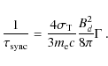
The typical Lorentz factor for the relativistic electrons radiating at frequency
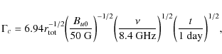
where we have used for the magnetic field configuration across the shock
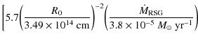
![$\displaystyle \bigg({u_w \over 10{\rm ~km~s}^{-1}}\bigg)^{-1} \bigg({B_{u0} \ov...
...)^{-1} \bigg({\nu \over 8.4~{\rm GHz}}\bigg)^{-1} \bigg]^{1/(2m-1)}~{\rm days}.$](/articles/aa/full_html/2009/19/aa11511-08/img300.png)
Here, we have used
4.3 Magnetic field amplification
Fransson & Björnsson (1998) modeled the radio emission of SN 1993J assuming that the radiation is emitted from a shell of uniform magnetic field. They found
![]() G (or alternatively
G (or alternatively
![]() G), which is in reasonable agreement with both our first estimate (Eq. (10)) and the mean postshock magnetic field resulting from our detailed analysis. Our best-fit value for the immediate postshock magnetic field is
G), which is in reasonable agreement with both our first estimate (Eq. (10)) and the mean postshock magnetic field resulting from our detailed analysis. Our best-fit value for the immediate postshock magnetic field is
![]() G, given
G, given
![]() (Fig. 5). The mean magnetic field strength in the synchrotron-emitting region is expected to be higher than Bd by a factor of less than two, given that the field is mainly advected in the downstream plasma (see Fig. 6), i.e.
(Fig. 5). The mean magnetic field strength in the synchrotron-emitting region is expected to be higher than Bd by a factor of less than two, given that the field is mainly advected in the downstream plasma (see Fig. 6), i.e.
![]() G. We note, however, that in our detailed model all the emitting electrons do not see the same mean magnetic field, because due to the energy losses the downstream transport of the nonthermal particles depends on the energy they acquired at the shock front.
G. We note, however, that in our detailed model all the emitting electrons do not see the same mean magnetic field, because due to the energy losses the downstream transport of the nonthermal particles depends on the energy they acquired at the shock front.
Pérez-Torres et al. (2001) were able to obtain a good fit to the radio light curves with
![]() G. But they did not take into account the electron energy losses and assumed the existence of a low-energy cutoff in the distribution of the relativistic particles, whose main effect is to flatten the radio light curves at the shortest wavelengths. But as discussed in Sect. 3.2, the observed flattening of the light curves at early epochs is naturally explained by the strong synchrotron losses suffered by the radiating electrons. Moreover, a low-energy cutoff in the particle distribution function is not supported by the DSA theory.
G. But they did not take into account the electron energy losses and assumed the existence of a low-energy cutoff in the distribution of the relativistic particles, whose main effect is to flatten the radio light curves at the shortest wavelengths. But as discussed in Sect. 3.2, the observed flattening of the light curves at early epochs is naturally explained by the strong synchrotron losses suffered by the radiating electrons. Moreover, a low-energy cutoff in the particle distribution function is not supported by the DSA theory.
As already pointed out by Fransson & Björnsson (1998) and Pérez-Torres et al. (2001) the magnetic field inferred from the radio observations is at least two orders of magnitude higher than the magnetic field of stellar origin that is expected to preexist in the wind of the red supergiant progenitor. The high magnetic field in the blast wave region is likely a result of an amplification associated with the production of nonthermal particles by nonlinear DSA. The diffusive streaming of cosmic-rays in the upstream plasma is expected to produce strong turbulence, which could amplify the chaotic component of the magnetic field (e.g., Bell & Lucek 2001; Amato & Blasi 2006; Vladimorov et al. 2006). Two different mechanisms of turbulence generation are discussed for SNR shocks. First, due to the cosmic-ray anisotropy in the shock precursor, a resonant instability is predicted to exist in this region and to produce a rapid and intense excitation of Alfvén waves (e.g., McKenzie & Völk 1982; Bell & Lucek 2001). Bell (2004) also found a nonresonant streaming instability caused by the Lorentz force associated with the cosmic-ray electric current, which could strongly amplified MHD perturbations of short wavelengths. The overall magnetic field amplification could be the result of both instabilities operating in the shock precursor.
The saturation value of the random magnetic field amplified by the nonresonant instability,
![]() ,
can be estimated from Eq. (28) of Pelletier
et al. (2006; see also Bell 2004):
,
can be estimated from Eq. (28) of Pelletier
et al. (2006; see also Bell 2004):
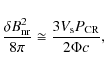
where
As previously stated (Sect. 2.3) the magnetic field evolution expected from the nonresonant instability mechanism uncovered by Bell (2004) is consistent with that inferred from the data. As shown in Fig. 15b, the strength of the field amplification calculated from Eq. (40) is also quite close to that required to explain the radio flux.
Following Pelletier et al. (2006) the relative importance of the resonant and nonresonant regimes of the streaming instability can be estimated from

This expression shows that in SN 1993J the nonresonant mechanism is expected to dominate at early times, but the resonant instability becomes more and more important as the shock is slowing down.
According to Bell (2004) the minimum timescale for growth of MHD waves driven by the nonresonant instability at a distance z upstream from the subshock is given by
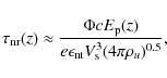
where -e is the electronic charge,
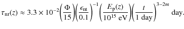
Thus, we have
![\begin{figure}
\par\includegraphics[width=9cm]{1511f15.eps}
\end{figure}](/articles/aa/full_html/2009/19/aa11511-08/img327.png) |
Figure 15:
a) Normalized immediate postshock pressures in thermal (
|
| Open with DEXTER | |
Because the damping of MHD turbulence can efficiently heat the thermal gas in the shock precursor region, a high amplification of the fluctuating magnetic field could at the same time provide a strong limitation for the modification of the shock structure induced by the cosmic-ray pressure. According to, e.g., Berezhko & Ellison (1999) the degree of heating of the shock precursor via Alfvén wave damping is set by the ratio
![]() (MS,u and
(MS,u and
![]() are the upstream sonic and Alfvén Mach numbers, respectively; see Sect. 2.4). Identifying Bu and
are the upstream sonic and Alfvén Mach numbers, respectively; see Sect. 2.4). Identifying Bu and
![]() one obtains from Eq. (41) the scaling relation
one obtains from Eq. (41) the scaling relation
which shows that for the same cosmic-ray pressure the shock modification should be less pronounced in a high-speed shock than in a slower one.
Björnsson & Fransson (2004) modeled the radio and X-ray emission from SN 2002ap with an accelerated electron energy index
![]() ,
as expected for a test-particle shock. The above scaling relation suggests that the absence of clear shock modification in this object is a consequence of the very high velocity of the blast wave (
,
as expected for a test-particle shock. The above scaling relation suggests that the absence of clear shock modification in this object is a consequence of the very high velocity of the blast wave (
![]() km s-1; Björnsson & Fransson 2004).
km s-1; Björnsson & Fransson 2004).
Various studies of the synchrotron emission produced in young SNRs led Berezhko & Völk (2006; see also Berezhko 2008) to propose the following empirical relation between the amplified magnetic field energy and the cosmic-ray pressure:
For SN 1993J, a better relation would be (see Eq. (40))
It is remarkable that this expression could provide a fair estimate of the magnetic field amplification in the high-speed blast wave of SN 1993J (
4.4 SN 1993J and the origin of cosmic rays
![\begin{figure}
\par\includegraphics[width=8.8cm]{1511f16.eps}
\end{figure}](/articles/aa/full_html/2009/19/aa11511-08/img337.png) |
Figure 16:
Maximum energy of shock-accelerated protons as a function of time after outburst.
|
| Open with DEXTER | |
As already pointed out by Bell & Lucek (2001) cosmic-rays were probably accelerated to very high energies in the blast wave of SN 1993J short after shock breakout. Calculated maximum proton energies are shown in Fig. 16. The quantity
![]() is the maximum energy caused by the finite age of the shock (Baring et al. 1999; Tatischeff & Hernanz 2007) and is obtained by time integration of the DSA rate from an initial acceleration time assumed to be t0=1 day after outburst. The maximum energy
is the maximum energy caused by the finite age of the shock (Baring et al. 1999; Tatischeff & Hernanz 2007) and is obtained by time integration of the DSA rate from an initial acceleration time assumed to be t0=1 day after outburst. The maximum energy
![]() is caused by the finite spatial extend of the shock and is calculated by equalling the upstream diffusion length of the accelerated protons to some fraction
is caused by the finite spatial extend of the shock and is calculated by equalling the upstream diffusion length of the accelerated protons to some fraction
![]() of the shock radius. Numerically, we find
(see, e.g., Tatischeff & Hernanz 2007)
of the shock radius. Numerically, we find
(see, e.g., Tatischeff & Hernanz 2007)
We see in Fig. 16 that for
In this context, it is instructive to estimate the total energy acquired by the cosmic-ray particles in SN 1993J during the early stage of interaction between the SN ejecta and the red supergiant wind:
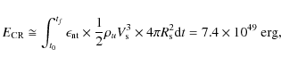
where tf=3100 days and
Most of the cosmic rays accelerated during this early stage were advected downstream from the shock and will remain inside the SNR until it merges with the interstellar medium. These particles suffer adiabatic losses and their energy decreases like
![]() (e.g. Drury 1996). Thus, they will make a negligible contribution to the interstellar cosmic-ray population at the end of the SNR. But as shown in Fig. 16, the highest-energy cosmic-rays are expected to escape continuously the shock system from upstream, due to the finite size of the acceleration region. The value obtained for
(e.g. Drury 1996). Thus, they will make a negligible contribution to the interstellar cosmic-ray population at the end of the SNR. But as shown in Fig. 16, the highest-energy cosmic-rays are expected to escape continuously the shock system from upstream, due to the finite size of the acceleration region. The value obtained for
![]() (Eq. (50)) suggests that these very-high energy particles could be important to the origin of interstellar cosmic rays above
(Eq. (50)) suggests that these very-high energy particles could be important to the origin of interstellar cosmic rays above
![]() eV.
eV.
At day ![]() 3100 after outburst, the blast wave started to expand into a more diluted CSM resulting from a lower mass loss rate of the SN progenitor more than
3100 after outburst, the blast wave started to expand into a more diluted CSM resulting from a lower mass loss rate of the SN progenitor more than ![]() 9000 years before explosion (see Weiler et al. 2007). The CSM density structure of SN 1993J can be explained by stellar evolution calculations that show that red supergiant stars can undergo a stage of intensified mass loss for few 104 years before SN explosion (Heger et al. 1997). After day
9000 years before explosion (see Weiler et al. 2007). The CSM density structure of SN 1993J can be explained by stellar evolution calculations that show that red supergiant stars can undergo a stage of intensified mass loss for few 104 years before SN explosion (Heger et al. 1997). After day
![]() 3100 post-outburst, an additional number of very-high energy cosmic-rays could have escaped the shock region into the interstellar medium, because their diffusion length
3100 post-outburst, an additional number of very-high energy cosmic-rays could have escaped the shock region into the interstellar medium, because their diffusion length ![]() has increased (
has increased (
![]() ;
see Eq. (41)). Significant variations in the mass loss activity of red supergiant stars prior to explosion are commonly inferred from radio observations of type II SNe (Weiler et al. 2002).
;
see Eq. (41)). Significant variations in the mass loss activity of red supergiant stars prior to explosion are commonly inferred from radio observations of type II SNe (Weiler et al. 2002).
These results suggest that Galactic cosmic rays of energies above
![]() eV could be produced immediately after the explosion of massive stars (Völk & Biermann 1988; Biermann 1993), provided that the acceleration efficiency found for SN 1993J is typical of most SNe and that the mass-loss rate obtained for the progenitor of this type IIb SN,
eV could be produced immediately after the explosion of massive stars (Völk & Biermann 1988; Biermann 1993), provided that the acceleration efficiency found for SN 1993J is typical of most SNe and that the mass-loss rate obtained for the progenitor of this type IIb SN,
![]() yr-1, is close to the mean mass-loss rate of red supergiant stars prior to explosion.
yr-1, is close to the mean mass-loss rate of red supergiant stars prior to explosion.
4.5 SN 1993J as a gamma-ray source
Kirk et al. (1995) pointed out that radio SNe could emit a large flux of very-high energy gamma rays arising from the decay of neutral pions created in hadronic collisions of cosmic rays with target nuclei. A detection of the predicted TeV emission with ground-based atmospheric Cherenkov telescopes would provide a direct confirmation of efficient acceleration of high-energy protons in SN explosions.
According to Kirk et al. (1995), SN 1993J was a promising target for detection, with a predicted flux of gamma-rays above 1 TeV of
![]() cm-2 s-1 for years after outburst. But their calculations assumed a much flatter CSM density profile,
cm-2 s-1 for years after outburst. But their calculations assumed a much flatter CSM density profile,
![]() ,
than the standard radial dependence
,
than the standard radial dependence
![]() found here.
found here.
The gamma-ray flux can be estimated from
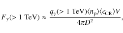
where
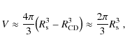
where
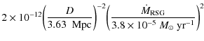

where we have used
But the TeV gamma-ray emission can be attenuated by the pair production process
![]() in the strong radiation field from the SN ejecta. The corresponding optical depth at the gamma-ray energy
in the strong radiation field from the SN ejecta. The corresponding optical depth at the gamma-ray energy ![]() can be estimated from
can be estimated from
where
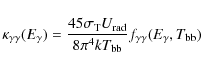
is the absorption coefficient in the diluted blackbody radiation field of temperature
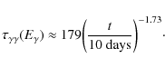
Thus, the early TeV emission of SN 1993J was strongly attenuated by photon-photon absorption. Multiplying the unabsorbed flux
Below ![]() 50 GeV, gamma rays are not attenuated by pair production in collisions with optical photons. The total gamma-ray flux in the energy range 1-50 GeV can be readily estimated from Eq. (51) using the emissivity
50 GeV, gamma rays are not attenuated by pair production in collisions with optical photons. The total gamma-ray flux in the energy range 1-50 GeV can be readily estimated from Eq. (51) using the emissivity
![]() photons s-1 erg-1 cm3 (H-atom)-1 (Drury et al. 1994). It gives for SN 1993J
photons s-1 erg-1 cm3 (H-atom)-1 (Drury et al. 1994). It gives for SN 1993J
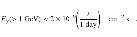
The mean flux of gamma rays above 1 GeV from day 1 to day 8 after outburst is then
5 Conclusions
Inspired by previous works on the morphology of synchrotron emission in Galactic SNRs (Cassam-Chenaï et al. 2005), I have employed a model to explain the radio emission of SN 1993J, which includes nonlinear effects of the diffusive shock acceleration mechanism. The model states that cosmic-ray ions are accelerated at the SN blast wave and their pressure modifies the shock structure. Therefore, the energy spectrum of the accelerated electrons depends on the rate of injection of shocked protons into the acceleration process. The nonthermal electrons suffer both adiabatic and radiative losses during their advection downstream the shock, which modify their energy distribution. The hydrodynamic evolution of the postshock plasma is calculated by assuming that the SN expansion is self-similar. The relativistic electrons emit synchrotron radiation in the ambient magnetic field and the corresponding radio emission is worked out from radiative transfer calculations that include the process of synchrotron self-absorption. The magnetic field amplification associated with the efficient production of cosmic-rays is not calculated in the framework of the model, but instead the strength of the amplified field is determined from a fit to the radio data. The model contains three other parameters to be fitted to the data: the shocked proton and electron injection rates into the DSA process and the mass loss rate of the SN progenitor.
The extensive radio observations of SN 1993J make this object a unique ``laboratory'' to study cosmic-ray acceleration in a SN shock. In particular, the VLBI imaging observations that resulted in detailed measurements of the SN expansion are of prime interest for the DSA theory. By applying the model to both the high-resolution brigthness profile at 3.6 cm measured by Biethenholz et al. (2003) and radio light curves at six frequencies reported by Weiler et al. (2007), I have obtained the following main conclusions:
- 1.
- The CSM density profile is consistent with a constant, steady wind of the red supergiant progenitor of the SN for
 9000 years before explosion. Contrary to previous claims, SN 1993J is not markedly different from the other studied radio SNe with regards to the mass loss evolution of the progenitor star. The best-fit mass-loss rate is
 yr-1 for the assumed stellar wind terminal velocity uw=10 km s-1 and CSM temperature
 K.
K.
- 2.
- The observed morphology of the radio emission provides evidence that part of the synchrotron radiation (
 17% of the total flux density at day 2787 post-outburst) is produced by electrons accelerated at the reverse shock.
- 3.
- The best-fit rate of injection of cosmic-ray protons into the DSA process at the forward shock is
 ,
with an estimated error of a factor of two. The calculated fraction of the total incoming energy flux converted by the blast wave to cosmic-ray energy during the first 8.5 years after explosion is
,
with an estimated error of a factor of two. The calculated fraction of the total incoming energy flux converted by the blast wave to cosmic-ray energy during the first 8.5 years after explosion is
 .
The shock modification induced by the backpressure from the accelerated ions is increasing with time after outburst. However, the cosmic-ray pressure accounts for less than 20% of the total postshock pressure at all times, such that the shock modification remains relatively weak.
.
The shock modification induced by the backpressure from the accelerated ions is increasing with time after outburst. However, the cosmic-ray pressure accounts for less than 20% of the total postshock pressure at all times, such that the shock modification remains relatively weak.
- 4.
- The best-fit cosmic-ray electron injection rate is
 and the calculated electron-to-proton density ratio at 10 GeV is
 .
The obtained value of
.
The obtained value of
 is lower than that measured in the Galactic cosmic-rays near Earth, 10-2. The latter number, however, results from cosmic-ray transport in the Galaxy and therefore is probably not indicative of the relativistic electron-to-proton ratio at the source of cosmic-ray acceleration.
- 5.
- The synchrotron energy losses suffered by the radiating electrons in the postshock magnetic field are important for the modeling of both the radio light curves and the morphology of the radio emission. The inferred magnetic field is broadly consistent with that expected from an amplification in the shock precursor region by the nonresonant regime of the cosmic-ray streaming instability. The magnetic field immediately upstream from the subshock is found to be
 with
with
 and
and
 G. The measured field strength is higher by a factor of 2 to 5 than the saturated value of the turbulent magnetic field predicted from the model of Bell (2004) for the turbulence generation. The energy density in the amplified magnetic field is found to obey the relation
- 6.
- The turbulent magnetic field amplified in the precursor region is not damped behind the shock (as proposed by Pohl et al. 2005, for Galactic SNRs) but essentially carried along by the plasma flow in the downstream region.
- 7.
- The magnetic field amplification increases the DSA rate, thus allowing the rapid acceleration of cosmic-ray protons to energies well above 1015 eV. The proton maximum energy is find to be limited by the finite confinement size of the shock, which implies that the highest-energy cosmic rays continuously escaped the acceleration region from upstream during the first 8.5 years after explosion. After that time, when the blast wave passed the limit of the dense CSM established by a stage of high mass loss from the red supergiant progenitor prior to explosion, an additional number of very-high energy protons probably escaped into the interstellar medium. The results obtained for this SN provide support to the model of Völk & Biermann (1988) and Biermann (1993) that the Galactic cosmic-rays above 1015 eV are accelerated in the explosion of massive stars, during the early stage of interaction of the SN ejecta with the progenitor wind.
- 8.
- The early emission from SN 1993J of TeV gamma-rays produced in hadronic collisions of accelerated cosmic-rays with ambient material was strongly attenuated by pair production in the dense radiation field from the SN ejecta. The flux at Earth of photons of energy above 1 TeV reached a maximum of only
 cm-2 s-1 at day 270 after explosion. Above 1 GeV, the flux is found to be
 cm-2 s-1. This result suggests that type II SNe could be detected in
  -decay gamma-rays with the Fermi Gamma-ray Space Telescope out to a maximum distance of only 1 Mpc.
Acknowledgements
It is a pleasure to thank Margarita Hernanz for numerous discussions and her hospitality at IEEC-CSIC, where most of this work has been done. I am greatly indebted to Jean-Pierre Thibaud for his generous and stimulating input throughout the writing of the paper. I am also greatful to Gamil Cassam-Chenaï, Anne Decourchelle, Jürgen Kiener, Alexandre Marcowith, and Régis Terrier for numerous illuminating discussions and to Roger Chevalier for his critical reading of the manuscript. Financial support from the Generalitat de Catalunya through the AGAUR grant 2006-PIV-10044 and the project SGR00378 is acknowledged.
Appendix A: Magnetic field evolution from the parametric model of Weiler et al.
Weiler et al. (1986,2002, and references therein) have developed a semi-phenomenological model to described the light curves of radio SNe. In this model, the flux density at a given frequency ![]() and time t after outburst can be expressed as
and time t after outburst can be expressed as
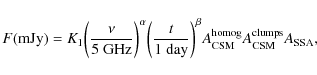
where
and
with
and
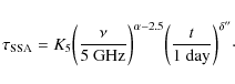
Here, K1 represents the unabsorbed flux density in mJy, and K2, K3, and K5 are the optical depths for attenuation by a homogeneous absorbing CSM, a clumpy or filamentary CSM, and internal SSA, respectively, at day one after outburst and for
We show here that an estimate of the mean magnetic field strength in the radio emission region,
![]() ,
can be obtained from a comparison of this parametric model with the SSA model of Chevalier (1998). In the latest formalism, the synchrotron emission is produced by relativistic electrons having a power-law energy distribution:
,
can be obtained from a comparison of this parametric model with the SSA model of Chevalier (1998). In the latest formalism, the synchrotron emission is produced by relativistic electrons having a power-law energy distribution:
![]() ,
where the spectral index
,
where the spectral index ![]() is independent of time. The emitting spherical shell is approximated by a planar region in the plane of the sky with an area
is independent of time. The emitting spherical shell is approximated by a planar region in the plane of the sky with an area ![]() ,
where R is the radius. In the absence of FFA by an external medium, the observable flux density can be written as
,
where R is the radius. In the absence of FFA by an external medium, the observable flux density can be written as
with
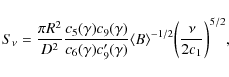
where D is the source distance, the constant
![\begin{displaymath}c'_9(\gamma)={\sqrt{\pi} \over 2} {\Gamma[(\gamma+6)/4]\over\Gamma[(\gamma+8)/4]},
\end{displaymath}](/articles/aa/full_html/2009/19/aa11511-08/img416.png)
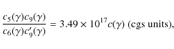
where the expression for
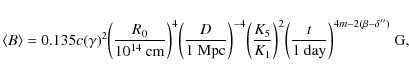
where we have identified the radius R with the forward shock radius
Table A.1:
Parameter ![]() for use in Eq. (A.12).
for use in Eq. (A.12).
Equation (A.12) can in principle provide an estimate of the mean magnetic field in the synchrotron-emitting region as a function of the fitted parameters K1, K5, ![]() ,
and
,
and
![]() .
But in the case of combined SSA and FFA, the result strongly depends on the FFA model, which is uncertain (Sect. 2.2). Thus, with the best-fit parameters
.
But in the case of combined SSA and FFA, the result strongly depends on the FFA model, which is uncertain (Sect. 2.2). Thus, with the best-fit parameters
![]() and
and
![]() obtained for SN 1993J by Weiler et al. (2007), one gets the unreasonable time dependence
obtained for SN 1993J by Weiler et al. (2007), one gets the unreasonable time dependence
![]() (for m=0.83). We argue in Sect. 4.3 that magnetic field amplification by cosmic-ray streaming should lead to
(for m=0.83). We argue in Sect. 4.3 that magnetic field amplification by cosmic-ray streaming should lead to
![]() with
with
![]() ,
as long as the shock is not strongly modified by the back pressure from the energetic ions. Thus, we expect the relation
,
as long as the shock is not strongly modified by the back pressure from the energetic ions. Thus, we expect the relation
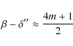
to hold in most of the cases. Using this constraint in the fitting procedure could allow to better determine the physical parameters of radio SNe, in particular the mass loss rate of the progenitor star.
Appendix B: Radiative transfer calculations
The synchrotron emission coefficient (in erg cm-3 s-1 sr-1 Hz-1) averaged over the pitch angle is given as a function of radius by (see, e.g., Pacholczyk 1970)
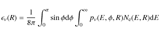
and the absorption coefficient (cm-1) by
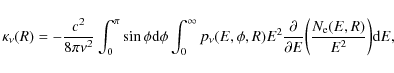
where
Here, -e is the electron charge, K5/3 the modified Bessel function, and
the critical frequency. In the computer code I have developed, the emission coefficient is calculated by numerical integration of Eq. (B.1) using the tabulation of Pacholczyk (1970) for the integral of the modified Bessel function. The absorption coefficient is obtained by approximating the electron energy distribution by a power law
The absorption coefficient can then be simplified to (Pacholczyk 1970; Longair 1994)
This approximation is used to speed up the computation time. Its accuracy has been checked by solving numerically Eq. (B.2).
The brightness profile,
![]() ,
where
,
where ![]() is the distance to the center of the disk resulting from the projection of the SNR onto the plane of the sky, is calculated from the source function
is the distance to the center of the disk resulting from the projection of the SNR onto the plane of the sky, is calculated from the source function
![]() by solving the standard transfer equation (Rybicki & Lightman 1979):
by solving the standard transfer equation (Rybicki & Lightman 1979):

where the optical depths to SSA are defined as
with
Finally, the total flux density is given by
This quantity is multiplied by the attenuation factor
References
- Aharonian, F., Akhperjanian, A. G., Bazer-Bachi, A. R., et al. (HESS Collaboration) 2006, A&A, 457, 899 (In the text)
- Amato, E., & Blasi, P. 2006, MNRAS, 371, 1251 [NASA ADS] [CrossRef] (In the text)
- Arnett, W. D. 1988, ApJ, 331, 377 [NASA ADS] [CrossRef] (In the text)
- Axford, W. I. 1994, ApJS, 90, 937 [NASA ADS] [CrossRef] (In the text)
- Baring, M. G., Ellison, D. C., Reynolds, S. P., Grenier, I. A., & Goret, P. 1999, ApJ, 513, 311 [NASA ADS] [CrossRef] (In the text)
- Bartel, N., Bietenholz, M. F., Rupen, M. P., et al. 1994, Nature, 368, 610 [NASA ADS] [CrossRef] (In the text)
- Bartel, N., Bietenholz, M. F., Rupen, M. P., et al. 2000, Science, 287, 112 [NASA ADS] [CrossRef] (In the text)
- Bartel, N., Bietenholz, M. F., Rupen, M. P., et al. 2002, ApJ, 581, 404 [NASA ADS] [CrossRef]
- Bartel, N., Bietenholz, M. F., Rupen, M. P., & Dwarkadas, V. V. 2007, ApJ, 668, 924 [NASA ADS] [CrossRef] (In the text)
- Bell, A. R. 2004, MNRAS, 353, 550 [NASA ADS] [CrossRef] (In the text)
- Bell , A. R., & Lucek, S. G. 2001, MNRAS, 327, 433 [NASA ADS] [CrossRef] (In the text)
- Berezhko, E. G. 2008, Adv. Space Res., 41, 429 [NASA ADS] [CrossRef] (In the text)
- Berezhko, E. G., & Ellison, D. C. 1999, ApJ, 526, 385 [NASA ADS] [CrossRef] (In the text)
- Berezhko, E. G., & Völk, H. J. 2006, A&A, 451, 981 [NASA ADS] [CrossRef] [EDP Sciences] (In the text)
- Biermann, P. L. 1993, A&A, 271, 649 [NASA ADS] (In the text)
- Bietenholz, M. F., Bartel, N., & Rupen, M. P. 2003, ApJ, 597, 374 [NASA ADS] [CrossRef] (In the text)
- Björnsson, C.-I., & Fransson, C. 2004, ApJ, 605, 823 [NASA ADS] [CrossRef] (In the text)
- Blasi, P., Gabici, S., & Vannoni, G. 2005, MNRAS, 361, 907 [NASA ADS] [CrossRef] (In the text)
- Cassam-Chenaï, G., Decourchelle, A., Ballet, J., & Ellison, D. C. 2005, A&A, 443, 955 [NASA ADS] [CrossRef] [EDP Sciences] (In the text)
- Cassam-Chenaï, G., Hughes, J. P., Ballet, J., & Decourchelle, A. 2007, ApJ, 665, 315 [NASA ADS] [CrossRef] (In the text)
- Cassam-Chenaï, G., Hughes, J. P., Reynoso, E. M., Badenes, C., & Moffett, D. 2008, ApJ, 680, 1180 [NASA ADS] [CrossRef] (In the text)
- Chevalier, R. A. 1982a, ApJ, 258, 790 [NASA ADS] [CrossRef] (In the text)
- Chevalier, R. A. 1982b, ApJ, 259, 302 [NASA ADS] [CrossRef] (In the text)
- Chevalier, R. A. 1983, ApJ, 272, 765 [NASA ADS] [CrossRef]
- Chevalier, R. A. 1996, in Radio Emission from the Stars and the Sun, ed. A. R. Taylor, & J. M. Paredes (San Francisco: ASP), 125 (In the text)
- Chevalier, R. A. 1998, ApJ, 499, 810 [NASA ADS] [CrossRef] (In the text)
- Chevalier, R. A., & Fransson, C. 2006, ApJ, 651, 381 [NASA ADS] [CrossRef] (In the text)
- Chevalier, R. A., Blondin, J. M., & Emmering, R. T. 1992, ApJ, 392, 118 [NASA ADS] [CrossRef] (In the text)
- Decourchelle, A. 2005, in X-Ray and Radio Connections, ed. L. O. Sjouwerman, & K. K. Dyer, Published electronically by NRAO, http://www.aoc.nrao.edu/events/xraydio (In the text)
- Decourchelle, A., & Ballet, J. 1994, A&A, 287, 206 [NASA ADS] (In the text)
- Decourchelle, A., Ellison, D. C., & Ballet, J. 2000, ApJ, 543, L57 [NASA ADS] [CrossRef] (In the text)
- Drury, L. O. 1996, Space Sci. Rev., 75, 269 [NASA ADS] [CrossRef] (In the text)
- Drury, L. O., Aharonian, F. A., & Völk, H. J. 1994, A&A, 287, 959 [NASA ADS] (In the text)
- Duffy, P., Ball, L., & Kirk, J. G. 1995, ApJ, 447, 364 [NASA ADS] [CrossRef] (In the text)
- Ellison, D. C., & Cassam-Chenaï, G. 2005, ApJ, 632, 920 [NASA ADS] [CrossRef] (In the text)
- Ellison, D. C., & Vladimirov, A. 2008, ApJ, 673, L47 [NASA ADS] [CrossRef] (In the text)
- Ellison, D. C., Berezhko, E. G., & Baring, M. G. 2000, ApJ, 540, 292 [NASA ADS] [CrossRef] (In the text)
- Ellison, D. C., Decourchelle, A., & Ballet, J. 2005, A&A, 429, 569 [NASA ADS] [CrossRef] [EDP Sciences] (In the text)
- Fransson, C., & Björnsson, C.-I. 1998, ApJ, 509, 861 [NASA ADS] [CrossRef] (In the text)
- Fransson, C., & Björnsson, C.-I. 2005, Cosmic Explosions, On the 10th Anniversary of SN1993J, IAU Coll., 192, 59 (In the text)
- Fransson, C., Lundqvist, P., & Chevalier, R. A. 1996, ApJ, 461, 993 [NASA ADS] [CrossRef] (In the text)
- Freedman, W. L., Hughes, S. M., Madore, B. F., et al. 1994, ApJ, 427, 628 [NASA ADS] [CrossRef] (In the text)
- Gould, R. J. 1975, ApJ, 196, 689 [NASA ADS] [CrossRef] (In the text)
- Gould, R. J., & Schréder, G. P. 1967, Phys. Rev., 155, 1404 [NASA ADS] [CrossRef] (In the text)
- Heger, A., Jeannin, L., Langer, N., & Baraffe, I. 1997, A&A, 327, 224 [NASA ADS] (In the text)
- Helder, E. A., & Vink, J. 2008, ApJ, 686, 1094 [NASA ADS] [CrossRef] (In the text)
- Hughes, J. P., Rakowski, C. E., & Decourchelle, A. 2000, ApJ, 543, L61 [NASA ADS] [CrossRef] (In the text)
- Immler, S., Aschenbach, B., & Wang, Q. D. 2001, ApJ, 561, L107 [NASA ADS] [CrossRef] (In the text)
- Iwamoto, K., Young, T. R., Nakasato, N., et al. 1997, ApJ, 477, 865 [NASA ADS] [CrossRef] (In the text)
- Jones, F. C., & Ellison, D. C. 1991, Space Sci. Rev., 58, 259 [NASA ADS] [CrossRef] (In the text)
- Jun, B.-I., & Norman, M. L. 1996, ApJ, 465, 800 [NASA ADS] [CrossRef] (In the text)
- Jun, B.-I., Norman, M. L., & Stone, J. M. 1995, ApJ, 453, 332 [NASA ADS] [CrossRef] (In the text)
- Kirk, J. G., Duffy, P., & Ball, L. 1995, A&A, 293, L37 [NASA ADS] (In the text)
- Lewis, J. R., Walton, N. A., Meikle, W. P. S., et al. 1994, MNRAS, 266, L27 [NASA ADS] (In the text)
- Longair, M. S. 1994, High Energy Astrophysics (Cambridge University press) (In the text)
- Malkov, M. A., & O'C Drury, L. 2001, Rep. Prog. Phys., 64, 429 [NASA ADS] [CrossRef] (In the text)
- Marcaide, J. M., Alberdi, A., Elosegui, P., et al. 1994, ApJ, 424, L25 [NASA ADS] [CrossRef] (In the text)
- Marcaide, J. M., Alberdi, A., Ros, E., et al. 1995, Science, 270, 1475 [NASA ADS] [CrossRef] (In the text)
- Marcaide, J. M., Alberdi, A., Ros, E., et al. 1997, ApJ, 486, L31 [NASA ADS] [CrossRef]
- Marcowith, A., Lemoine, M., & Pelletier, G. 2006, A&A, 453, 193 [NASA ADS] [CrossRef] [EDP Sciences] (In the text)
- McKenzie, J. F., & Völk, H. J. 1982, A&A, 116, 191 [NASA ADS] (In the text)
- Mioduszewski, A. J., Dwarkadas, V. V., & Ball, L. 2001, ApJ, 562, 869 [NASA ADS] [CrossRef] (In the text)
- Morlino, G., Amato, E., & Blasi, P. 2009, MNRAS, 392, 240 [NASA ADS] [CrossRef] (In the text)
- Nadyozhin, D. K. 1985, Ap&SS, 112, 225 [NASA ADS] [CrossRef] (In the text)
- Natta, A., & Panagia, N. 1984, ApJ, 287, 228 [NASA ADS] [CrossRef] (In the text)
- Pacholczyk, A. G. 1970, Radio Astrophysics (San Francisco: Freeman) (In the text)
- Parizot, E., Marcowith, A., Ballet, J., & Gallant, Y. A. 2006, A&A, 453, 387 [NASA ADS] [CrossRef] [EDP Sciences] (In the text)
- Pelletier, G., Lemoine, M., & Marcovith, A. 2006, A&A, 453, 181 [NASA ADS] [CrossRef] [EDP Sciences] (In the text)
- Pérez-Torres, M. A., Alberdi, A., & Marcaide, J. M. 2001, A&A, 374, 997 [NASA ADS] [CrossRef] [EDP Sciences] (In the text)
- Pohl, M., Yan, H., & Lazarian, A. 2005, ApJ, 626, L101 [NASA ADS] [CrossRef] (In the text)
- Reynolds, S. P. 1998, ApJ, 493, 375 [NASA ADS] [CrossRef] (In the text)
- Richmond, M. W., Treffers, R. R., Filippenko, A. W., et al. 1994, AJ, 107, 1022 [NASA ADS] [CrossRef] (In the text)
- Ripero, J., Garcia, F., Rodriguez, D., et al. 1993, IAU Circ., 5731, 1 (In the text)
- Rybicki, G. B., & Lightman, A. P. 1979, Radiative Processes in Astrophysics (New York: Wiley) (In the text)
- Shigeyama, T., Suzuki, T., Kumagai, S., et al. 1994, ApJ, 420, 341 [NASA ADS] [CrossRef] (In the text)
- Soderberg, A. M., Kulkarni, S. R., Berger, E., et al. 2005, ApJ, 621, 908 [NASA ADS] [CrossRef] (In the text)
- Soderberg, A. M., Berger, E., Page, K. L., et al. 2008, Nature, 453, 469 [NASA ADS] [CrossRef] (In the text)
- Tatischeff, V. 2008, in Proc. of Supernovae: lights in the darkness (XXIII Trobades Cientifiques de la Mediterrania), PoS(028) [arXiv:0804.1004] (In the text)
- Tatischeff, V., & Hernanz, M. 2007, ApJ, 663, L101 [NASA ADS] [CrossRef] (In the text)
- Tran, H. D., Filippenko, A. V., Schmidt, G. D., et al. 1997, PASP, 109, 489 [NASA ADS] [CrossRef] (In the text)
- Uchiyama, Y., Aharonian, F. A., Tanaka, T., Takahashi, T., & Maeda, Y. 2007, Nature, 449, 576 [NASA ADS] [CrossRef] (In the text)
- Van Dyk, S. D., Weiler, K. W., Sramek, R. A., Rupen, M. P., & Panagia, N. 1994, ApJ, 432, L115 [NASA ADS] [CrossRef] (In the text)
- Vladimirov, A., Ellison, D. C., & Bykov, A. 2006, ApJ, 652, 1246 [NASA ADS] [CrossRef] (In the text)
- Völk, H. J., & Biermann, P. L. 1988, ApJ, 333, L65 [NASA ADS] [CrossRef] (In the text)
- Völk, H. J., Berezhko, E. G., Ksenofontov, L. T., & Rowell, G. P. 2002, A&A, 396, 649 [NASA ADS] [CrossRef] [EDP Sciences] (In the text)
- Völk, H. J., Berezhko, E. G., & Ksenofontov, L. T. 2005, A&A, 433, 229 [NASA ADS] [CrossRef] [EDP Sciences] (In the text)
- Warren, J. S., Hughes, J. P., Badenes, C., et al. 2005, ApJ, 634, 376 [NASA ADS] [CrossRef] (In the text)
- Weiler, K. W., Sramek, R. A., Panagia, N., van der Hulst, J. M., & Salvati, M. 1986, ApJ, 301, 790 [NASA ADS] [CrossRef] (In the text)
- Weiler, K. W., Panagia, N., & Sramek, R. A. 1990, ApJ, 364, 611 [NASA ADS] [CrossRef] (In the text)
- Weiler, K. W., Panagia, N., Montes, M. J., & Sramek, R. A. 2002, ARA&A, 40, 387 [NASA ADS] [CrossRef]
- Weiler, K. W., Williams, C. L., Panagia, N., et al. 2007, ApJ, 671, 1959 [NASA ADS] [CrossRef] (In the text)
- Wheeler, J. C., Barker, E., Benjamin, R., et al. 1993, ApJ, 417, L71 [NASA ADS] [CrossRef] (In the text)
- Young, T. R., Baron, E., & Branch, D. 1995, ApJ, 449, L51 [NASA ADS] [CrossRef] (In the text)
Footnotes
- ... France
![[*]](/icons/foot_motif.png)
- Permanent address.
- ... frequency
- This frequency dependence may explain why the outer radii obtained by Bartel et al. (2002) at 2.3 and 1.7 GHz tend to be larger by up to 5% than those measured by the same authors at higher frequencies.
- ... shocked
- We note that in Reynolds (1998) a factor
 is missing in Eq. (25) and in the unnumbered equation just before Eq. (24).
- ... wave
- In contrast, the radio morphology of older SNRs, such as Tycho's remnant, also depends on the proton injection parameter,
 ,
because in these objects an increase in the injection efficiency produces a narrower interaction region (Cassam-Chenaï et al. 2007). This is not the case in SN 1993J because of the much higher magnetic field strength in the shock precursor region, which limits the backreaction of the shock-accelerated nuclei on the shock structure (see Sect. 2.4).
,
because in these objects an increase in the injection efficiency produces a narrower interaction region (Cassam-Chenaï et al. 2007). This is not the case in SN 1993J because of the much higher magnetic field strength in the shock precursor region, which limits the backreaction of the shock-accelerated nuclei on the shock structure (see Sect. 2.4).
- ...

- These high values of
 are partly due to a few data points that strongly deviate from neighbouring points and appear to be incompatible with the general trend observed at each wavelength.
- ... uncertain
- A simple estimate of
 may be derived by assuming that the upstream escape boundary at
 corresponds to the distance for which the MHD growth timescale
 .
We then obtain from Eq. (43)
.
We then obtain from Eq. (43)
For ,
,
 ,
,
 ,
m=0.83, and
,
m=0.83, and
 (see above), we get
 .
However, the full interpretation of this result is beyond the scope of this paper.
.
However, the full interpretation of this result is beyond the scope of this paper.
- ... mode
- As calculated with the LAT source detectability tool at http://fermi.gsfc.nasa.gov/ssc/proposals/detectability.html
- ...1994)
- These quantities were not taken into account by Chevalier (1998), who made the approximation of replacing
 by
by
 .
.
All Tables
Table A.1:
Parameter ![]() for use in Eq. (A.12).
for use in Eq. (A.12).
All Figures
| |
Figure 1: Time evolution of the outer angular radius of the shell-like radio emission from SN 1993J. The data were obtained by Bartel et al. (2002) from observations at 1.7, 2.3, 5.0, 8.4, 14.8, and 22.2 GHz. The dotted line is a least-squares power-law fit to the data (Eq. (1)). |
| Open with DEXTER | |
| In the text | |
| |
Figure 2: Radio light curves for SN 1993J at 0.3, 1.2, 2, 3.6, 6, and 20 cm. The data are from Weiler et al. (2007) and references therein. The solid lines represent the best-fit semi-empirical model of these authors. The dotted lines show a synchrotron self-absorption (SSA) model in which the SSA optical depth and the unabsorbed flux density were obtained from fits to radio spectra taken between day 75 and day 923 after outburst (see Sect. 2.3). The difference between the latter model and the data before day 100 is partly due to free-free absorption of the radio emission in the CSM. |
| Open with DEXTER | |
| In the text | |
| |
Figure 3:
Evolution of the parameters
|
| Open with DEXTER | |
| In the text | |
| |
Figure 4:
Shocked proton and electron phase-space distributions vs. kinetic energy, at day 1000 after shock breakout. Following Berezhko & Ellison (1999), the phase-space distribution functions have been multiplied by
|
| Open with DEXTER | |
| In the text | |
| |
Figure 5:
Subshock and total compression ratios at the forward shock ( left axis) and nonthermal energy fraction
|
| Open with DEXTER | |
| In the text | |
| |
Figure 6:
Radial profiles of a) the gas density and b) the total magnetic field in the shock region. The density is normalized to the upstream value
|
| Open with DEXTER | |
| In the text | |
| |
Figure 7:
Relative brightness of the 3.6 cm emission from SN 1993J at day 2787 after outburst, as a function of angular radius. In the calculations, the outer angular radius |
| Open with DEXTER | |
| In the text | |
| |
Figure 8:
Calculated radial profiles of the relative emissivity at 3.6 cm and
|
| Open with DEXTER | |
| In the text | |
| |
Figure 9:
Same as Fig. 7 but for Bu0=30 G,
|
| Open with DEXTER | |
| In the text | |
| |
Figure 10:
Same as Fig. 7 but for the damping of the magnetic turbulence downstream ( green dashed lines) compared to the advection of the shocked plasma ( blue solid lines). In both cases, Bu0=50 G and
|
| Open with DEXTER | |
| In the text | |
| |
Figure 11:
Radio light curves for SN 1993J at 0.3, 1.2, 2, 3.6, 6, and 20 cm. The data are from Weiler et al. (2007) and references therein. The blue solid lines represent the best-fit model, which is obtained for
|
| Open with DEXTER | |
| In the text | |
| |
Figure 12:
Radio light curves of SN 1993J with the flux density multiplied by
|
| Open with DEXTER | |
| In the text | |
| |
Figure 13:
Same as Fig. 12 but for various values of the injection parameters:
|
| Open with DEXTER | |
| In the text | |
| |
Figure 14:
Same as Fig. 11 but for a CSM density profile of the form
|
| Open with DEXTER | |
| In the text | |
| |
Figure 15:
a) Normalized immediate postshock pressures in thermal (
|
| Open with DEXTER | |
| In the text | |
| |
Figure 16:
Maximum energy of shock-accelerated protons as a function of time after outburst.
|
| Open with DEXTER | |
| In the text | |
Copyright ESO 2009
Current usage metrics show cumulative count of Article Views (full-text article views including HTML views, PDF and ePub downloads, according to the available data) and Abstracts Views on Vision4Press platform.
Data correspond to usage on the plateform after 2015. The current usage metrics is available 48-96 hours after online publication and is updated daily on week days.
Initial download of the metrics may take a while.