| Issue |
A&A
Volume 499, Number 1, May III 2009
|
|
|---|---|---|
| Page(s) | 337 - 345 | |
| Section | Astronomical instrumentation | |
| DOI | https://doi.org/10.1051/0004-6361/200811506 | |
| Published online | 08 April 2009 | |
Roughness scattering in X-ray grazing-incidence telescopes
F. E. Zocchi
Media Lario Technologies, Località Pascolo, 23842 Bosisio Parini (LC), Italy
Received 11 December 2008 / Accepted 26 February 2009
Abstract
In the framework of the scalar theory of diffraction, we determine the rms width of the angle spread function degraded by surface roughness in reflective grazing-incidence optics of cylindrical symmetry for X-ray astronomy. Our derivation does not rely on the small roughness approximation, is thus valid for arbitrary roughness values, and takes into full consideration the cylindrical symmetry of the mirrors. The dependence of the rms beam width on both the grazing-incidence angles and the radiation wavelength is studied for both single and double reflection optics, the latter being more relevant to X-ray telescopes. When the small roughness approximation is applicable, we also derive an expression for the angle spread function of the optical system in the presence of roughness scattering that provides the correct expression for the rms beam width.
Key words: X-rays: general - telescopes - scattering
1 Introduction
A factor limiting the resolution of grazing-incidence optics for X-ray astronomy is the scattering caused by the surface roughness of the telescope mirrors. A number of X-ray space missions (Pareschi & Ferrando 2005; Gondoin et al. 1994; Bookbinder et al. 2008; Citterio et al. 1988; Friedrich et al. 2008; Aschenbach 1988; Weisskopf et al. 2000; Gehrels et al. 2004) have stimulated both theoretical and experimental research (Church & Takacs 1993; Spiller 1994; Harvey 1995a; Karabacak et al. 2000; Stearns et al. 1998; Harvey 1995b; Zhao & Spreybroeck 2003; Harvey et al. 1996; Church & Takacs 1995; Christensen et al. 1988) to understand and characterize in a more robust way the scattering of electromagnetic waves from rough surfaces. The typical resolution requirement at the focal plane of an X-ray telescope is sharper than 20 half energy width at X-ray photon energy between 0.1 and 80 , depending on the mission (Friedrich et al. 2008; Pareschi & Ferrando 2005; Gondoin et al. 1994), and at a grazing-incidence angle in the range between about 0.1 and 1.5. Consequently, the contribution of roughness to the overall optical resolution is sufficiently low to require reflective surfaces polished down to roughness of about 0.2 ![]() 0.5 rms, typically in the spatial frequency range between 0.01 and 1. Hence, the correlation between surface roughness and radiation scattering is essential to defining the surface quality required by the mirrors.
0.5 rms, typically in the spatial frequency range between 0.01 and 1. Hence, the correlation between surface roughness and radiation scattering is essential to defining the surface quality required by the mirrors.
The interest in the field has been further boosted by other applications of the short-wavelength region of the electromagnetic spectrum, including EUV microlithography (Schellenberg 2008; Bakshi 2008) and EUV microscopy (Foltyn et al. 2004; Silk 1980; Schäfer et al. 2006), just to quote a few. The development of multilayer structures (Spiller 2003; Joensen et al. 1995; Barbee 1986; Yamashita et al. 1999) to enhance the optical reflectivity of mirrors at short wavelengths has also stimulated theoretical and experimental investigations in the field.
The configuration of choice for the optical design of X-ray telescopes is based on the type I Wolter architecture (Wolter 1952b) in which the X-ray radiation from distant sources is first reflected by a parabolic surface and then by a hyperboloid, both with cylindrical symmetry around the optical axis. The two surfaces are arranged in a coaxial configuration and share a common focus. The second focus of the hyperboloid is the image focus. To maximize the energy throughput, the telescope consists of a multitude of these double-reflection mirrors arranged in a nested configuration. All mirrors operate at grazing-incidence angles low enough to assure high reflectivity from the coating material at X-ray wavelengths. A mirror based on the Wolter architecture is known to satisfy approximately Abbe's condition (Braat 1997; Abbe 1873), assuring limited coma aberration for moderate field of view. A variation of the Wolter telescope, the Wolter-Schwarzschild configuration (Chase & Speybroeck 1973; Wolter 1952a), exactly satisfies Abbe's condition. Other designs are possible (Zocchi & Vernani 2007; Giacconi et al. 1969) but they all share the double-reflection feature at very small grazing-incidence angle.
Although a significant number of scientific publications have appeared in which the degradation of the performance of optical systems by scattering from surface roughness has been analyzed, the theoretical determination of the angular width of the scattered beam has received much less attention. The relation between the half-energy width in grazing-incidence telescopes and the roughness variance was studied in (Spiga 2007) by applying the Debye-Waller expression for the total integrated scattering (Spiller 1994) in 1-dimensional geometry. In the framework of the scalar theory of diffraction (Gaskill 1978; Born & Wolf 1980; Goodman 1968; Harvey 1995b), an exact derivation of the rms width of the angle spread function from the corresponding optical transfer function (Harvey et al. 1988; Gaskill 1978; Born & Wolf 1980; Goodman 1968; Smith 1963) in 2-dimensional geometry was reported in (Zocchi 2009), in which the contribution of scattering to the rms width of the angle spread function was shown to depend on only the variance of the roughness slope. However, even in these two papers (Spiga 2007; Zocchi 2009), the cylindrical symmetry of an X-ray telescope was not taken into account.
In this work, the rms width of the angle spread function of grazing-incidence optics with cylindrical symmetry is derived for arbitrary values of the roughness variance in the framework of the scalar theory of Fourier diffraction. In the following, we simply refer to the rms width of the angle spread function as the beam width. No further approximations are introduced into the derivation apart from the assumption that the angle between the axial profile of the optics and the optical axis is small. It is found again that the contribution of scattering to the width of the angle spread function depends only on the variance of the roughness slope. However, in the extreme case in which both the tapering angle of the optics and the grazing-incidence angle are small, the proportionality factor between the roughness slope and the beam width is half of that found for the reflection on an almost flat surface.
When the small roughness approximation is valid, it is also shown that the angle spread function can be written in a standard form as the convolution of the angle spread function of a perfectly smooth optics with an effective power spectral density expressed by a line integral of the true power spectral density of surface roughness of the mirrors. Finally, for an isotropic power-law dependence of the power spectral density on the spatial frequency, the behavior of the beam width as a function of the radiation wavelength ![]() and the grazing-incidence angle
and the grazing-incidence angle ![]() is also studied. If m is the exponent of the power-law power spectral density, the contribution of scattering to the beam width is proportional to
is also studied. If m is the exponent of the power-law power spectral density, the contribution of scattering to the beam width is proportional to
![]() .
.
The paper is organized as follows. Section 2 briefly reviews the standard approach used to derive the angle spread function of a rough mirror in the framework of Fourier optics within the small angle approximation, when the angle between the principal ray and any other rays in the optical system is small. This approximation limits the application to mirrors of low ratio of the diameter to the radius of curvature. The results and methods summarized in Sect. 2 are then used in Sect. 3 to derive the width of the angle spread function in grazing-incidence optics with cylindrical symmetry. Finally, in Sect. 4 we derive an expression for the angle spread function when the small roughness approximation is valid. In this last section, the dependence of the beam width on the radiation wavelength and the grazing-incidence angle is also studied for an isotropic surface characterized by a power-law expression for the power spectral density. The paper ends with two Appendixes. The first presents some mathematical derivations, and in the second we discuss the range of validity of Fourier optics treatment of scattering from surface roughness, and consequently of the content of this paper, and its relation to the small roughness approximation.
2 Angle spread function of rough optics
In this section, we briefly review the treatment of radiation scattering from surface roughness in the framework of the scalar theory of diffraction (Harvey et al. 1988; Gaskill 1978; Born & Wolf 1980; Goodman 1968; Smith 1963). In this theory, the optical transfer function
![]() of the imaging system is given by the normalized autocorrelation of the generalized complex pupil function
of the imaging system is given by the normalized autocorrelation of the generalized complex pupil function
![]() in the exit pupil plane (Harvey 1995b; Stearns et al. 1998),
in the exit pupil plane (Harvey 1995b; Stearns et al. 1998),
where
where
where r1 and r2 are the components of
![$\displaystyle H(\vec{f})= \int A_{0}(\vec{r})A_{0}^{*}(\vec{r}+ \lambda \vec{f}...
...n \theta}},r_{2}+ \lambda f_{2} \right) \right]} \right\rangle {\rm d} \vec{r}.$](/articles/aa/full_html/2009/19/aa11506-08/img19.png)
The final step consists in assuming that
![\begin{displaymath}
\left\langle {\rm e}^{\frac{\scriptstyle{4 \pi {\rm i} \sin ...
...}}{\scriptstyle{\sin \theta}}, \lambda f_{2} \right) \right]},
\end{displaymath}](/articles/aa/full_html/2009/19/aa11506-08/img20.png)
where
![\begin{displaymath}
H(\vec{f})=H_{0}(\vec{f}) {\rm e}^{- \frac{\scriptstyle{16 \...
...}}{\scriptstyle{\sin \theta}}, \lambda f_{2} \right) \right]},
\end{displaymath}](/articles/aa/full_html/2009/19/aa11506-08/img23.png)
where
![\begin{figure}
\par\includegraphics[width=14cm,clip]{1506Fig1.ps}
\end{figure}](/articles/aa/full_html/2009/19/aa11506-08/img25.png) |
Figure 1: Geometry of the grazing-incidence optics with cylindrical symmetry: conceptual 3D drawing ( left) anf optics cross section ( right). |
| Open with DEXTER | |
The inverse Fourier transform of the optical transfer function is the angle spread function (Harvey 1995b). When dealing with scattering phenomena, the use of the angle spread function is more convenient than the point spread function since the former is also applicable to large scattering angles (Harvey 1995a,b). In this formalism, the Fourier variable conjugate to the dimensionless frequency vector ![]() appearing in Eq. (6) is the vector of direction cosines
appearing in Eq. (6) is the vector of direction cosines
![]() of components
of components
![]() and
and
![]() in the image plane. Because of the Fourier transform relation between the optical transfer function
in the image plane. Because of the Fourier transform relation between the optical transfer function
![]() and the angle spread function
and the angle spread function
![]() ,
the integral of the latter is normalized to unity,
,
the integral of the latter is normalized to unity,
The integration in the above equation should be performed in the domain
where the first equality follows by taking into account the expression
The width of the reflected and scattered beam can be defined to be the root mean square value of the scattering angle weighted by the angle spread function,
The full angular width of the beam is then
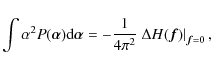
where
The right-hand side of Eq. (9) can be calculated in terms of
where
are the variances of roughness slope along the direction of the incidence plane and normal to the incidence plane, respectively. In Eq. (10),
3 Width of the angle spread function in X-ray telescopes
The results presented in the previous section are valid for almost flat mirrors. The theory is now extended to the case of grazing-incidence optics with cylindrical symmetry. We still assume the validity of the small angle approximation: in each plane containing the optical axis, the angle between any two rays reflected along a mirror profile is much smaller than the average grazing-incidence angle.
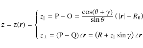
The analysis is based on the geometry shown in Fig. 1. It is assumed that the grazing-incidence optics consists of a mirror with just one reflection that can be approximated by a cone forming an angle ![]() with the optical axis. The extension to two or more reflections will be considered later. The rays reflected from the optics form a grazing-incidence angle
with the optical axis. The extension to two or more reflections will be considered later. The rays reflected from the optics form a grazing-incidence angle ![]() with the optical surface and are contained in planes through the optical axis. The exit pupil plane is perpendicular to the optical axis, which is also the axis of the cone. The largest radius R of the cone is projected onto the exit pupil plane as a circle of radius R0. The position on the optical surface is defined by a coordinate z|| along a profile of the cone and a coordinate
with the optical surface and are contained in planes through the optical axis. The exit pupil plane is perpendicular to the optical axis, which is also the axis of the cone. The largest radius R of the cone is projected onto the exit pupil plane as a circle of radius R0. The position on the optical surface is defined by a coordinate z|| along a profile of the cone and a coordinate ![]() along circles at the intersection of the optical surface with planes normal to the optical axis. In addition, we form the vector
along circles at the intersection of the optical surface with planes normal to the optical axis. In addition, we form the vector ![]() of components z|| and
of components z|| and ![]() .
We use polar coordinates in the pupil plane: with a point in this plane identified by a position vector
.
We use polar coordinates in the pupil plane: with a point in this plane identified by a position vector ![]() ,
we associate its modulus r and its anomaly
,
we associate its modulus r and its anomaly ![]() .
We finally assume that the pupil function
.
We finally assume that the pupil function
![]() has cylindrical symmetry and depends only on the modulus r of
has cylindrical symmetry and depends only on the modulus r of ![]() .
.
The relation
![]() between the vector
between the vector ![]() on the optical surface and the vector
on the optical surface and the vector ![]() on the pupil plane is obtained by inspection of Fig. 1 as
on the pupil plane is obtained by inspection of Fig. 1 as
The analysis is much simpler if we assume that the angle
where
![\begin{displaymath}
H(\vec{f})= \int A_{0}(r)A_{0}^{*} \left( \left\vert \vec{r}...
...ambda \vec{f}) \right) \right]} \right\rangle {\rm d} \vec{r}.
\end{displaymath}](/articles/aa/full_html/2009/19/aa11506-08/img63.png)
By assuming that the angle
![\begin{displaymath}
H(\vec{f})= \int A_{0}(r)A_{0}^{*} \left( \left\vert \vec{r}...
...ta \vec{z} (\vec{r},\vec{f}) \right) \right]} {\rm d} \vec{r},
\end{displaymath}](/articles/aa/full_html/2009/19/aa11506-08/img64.png)
where
![$\displaystyle R \arccos \left[ \frac{\vec{r} \cdot (\vec{r}+ \lambda \vec{f})}{r \left\vert \vec{r}+ \lambda \vec{f} \right\vert} \right].$](/articles/aa/full_html/2009/19/aa11506-08/img71.png)
Equation (18) is valid when the anomaly of
An important conclusion can be derived from Eqs. (16)-(18). Since the pupil function A0(r) has cylindrical symmetry, the dependence of the integrand on the anomaly
![]() of the vector
of the vector ![]() is expressed by the scalar product
is expressed by the scalar product
![]() or, equivalently, by the function
or, equivalently, by the function
![]() .
By making the change of integration variable
.
By making the change of integration variable
![]() ,
we see that the optical transfer function depends only on the modulus f of the vector
,
we see that the optical transfer function depends only on the modulus f of the vector ![]() and, consequently, has cylindrical symmetry. We note that no assumptions have been made about the isotropy of the roughness covariance
and, consequently, has cylindrical symmetry. We note that no assumptions have been made about the isotropy of the roughness covariance
![]() .
Regardless of the angular dependence of
.
Regardless of the angular dependence of
![]() ,
the optical transfer function and angle spread function inherit the cylindrical symmetry of the optics geometry.
,
the optical transfer function and angle spread function inherit the cylindrical symmetry of the optics geometry.
A further observation can be made about the power spectral density of surface roughness. Since the covariance function is a periodic function of ![]() of period
of period ![]() ,
the power spectral density
,
the power spectral density
![]() is discrete in the conjugate variable
is discrete in the conjugate variable
![]() .
Only multiple values of
.
Only multiple values of
![]() are allowed. However, this has limited practical implications since at this spatial frequency the entire formalism in which roughness is considered to be a stationary stochastic process breaks down. The theory is only applicable at spatial frequencies much higher than
are allowed. However, this has limited practical implications since at this spatial frequency the entire formalism in which roughness is considered to be a stationary stochastic process breaks down. The theory is only applicable at spatial frequencies much higher than
![]() .
.
According to Eq. (9), to calculate the width of the angle spread function, we must evaluate the value of the Laplacian of the optical transfer function with respect to ![]() at the origin. This calculation is simplified by noting that the gradient
at the origin. This calculation is simplified by noting that the gradient
![]() vanishes at the origin, as shown in Appendix A. By taking into account that
vanishes at the origin, as shown in Appendix A. By taking into account that
![]() and
H0(0)=1, it follows from Eq. (16) that
and
H0(0)=1, it follows from Eq. (16) that
The first integral in Eq. (19) is simply
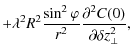
where
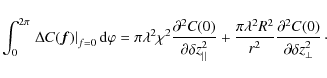
The second derivatives at the origin of
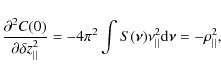
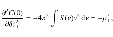
where
![$\displaystyle \times \left[ \chi^{2} \rho_{\vert\vert}^{2} \int_{0}^{\infty} \l...
...}^{\infty} \frac{\left\vert A_{0}(r) \right\vert^{2}}{r} {\rm d} r \right]\cdot$](/articles/aa/full_html/2009/19/aa11506-08/img105.png)
The first integral in Eq. (24), multiplied by

![$\displaystyle \frac{\ln \left[ \vphantom{\rule{0pt}{8pt}} (R_{0}+d_{0})/R_{0} \right]}{\pi d_{0}(2R_{0}+d_{0})}\cdot$](/articles/aa/full_html/2009/19/aa11506-08/img111.png)
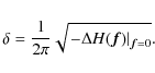
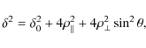
By combining Eqs. (9), (24), and (25), the width of the angle spread function becomes
![\begin{displaymath}
\delta^{2}= \delta_{0}^{2}+2 \rho_{\vert\vert}^{2} \cos^{2}(...
...0pt}{8pt}} (R_{0}+d_{0})/R_{0} \right]} {d_{0}(2R_{0}+d_{0})},
\end{displaymath}](/articles/aa/full_html/2009/19/aa11506-08/img112.png)
where we have taken into account that
to first order in d0/R0. Equation (27) is independent of d0. When both
By comparison with Eq. (10), we note that the contribution of roughness to the width of the angle spread function is half that found for the reflection on an almost flat surface.
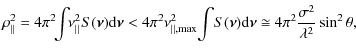
As an example, we determine the roughness contribution
![]() to the rms beam width
to the rms beam width ![]() in the case of a single reflection mirror with surface roughness described by the isotropic power spectral density
in the case of a single reflection mirror with surface roughness described by the isotropic power spectral density
![]() (Church 1988). If
(Church 1988). If ![]() is the half field of view, the cut-off spatial frequencies in Eqs. (22) and (23) are
is the half field of view, the cut-off spatial frequencies in Eqs. (22) and (23) are
![]() along the direction of the optical axis and
along the direction of the optical axis and
![]() along the curved orthogonal direction, respectively. Here we assume that
along the curved orthogonal direction, respectively. Here we assume that ![]() and
and
![]() .
Equations (22) and (23) then imply that
.
Equations (22) and (23) then imply that

where we applied the change of integration variable
For
The extension of Eq. (27) to multiple uncorrelated surfaces is straightforward since the integrand in Eq. (16) is simply multiplied by an exponential factor for each surface (Stearns et al. 1998). In the presence of N surfaces, each of roughness covariance
![]() ,
variance
,
variance
![]() ,
slope variances
,
slope variances
![]() and
and
![]() ,
incidence angle
,
incidence angle
![]() ,
tapering angle
,
tapering angle
![]() ,
and scaling factor gk, the optical transfer function becomes
,
and scaling factor gk, the optical transfer function becomes
![$\displaystyle H(f)= \! \! \int \! A_{0}(r)A_{0}^{*} \left( \left\vert \vec{r}+ ...
...pt}{6pt}} \delta \vec{z}_{k}(\vec{r},\vec{f}) \right) \right]} {\rm d} \vec{r},$](/articles/aa/full_html/2009/19/aa11506-08/img143.png)
and the beam width is now
4 Approximation of the angle spread function
Equation (16) defines the optical transfer function as a complicated integral of the pupil function and the roughness covariance. In this section, we first develop a simpler approximation of the optical transfer function that provides the same expression as Eq. (27) for the beam width ![]() .
In the small roughness approximation, we also derive the angle spread function and express it in terms of an effective power spectral density obtained from the roughness power spectral density. Finally, the dependence of the rms beam width on the radiation wavelength and the grazing-incidence angle is studied in more detail.
.
In the small roughness approximation, we also derive the angle spread function and express it in terms of an effective power spectral density obtained from the roughness power spectral density. Finally, the dependence of the rms beam width on the radiation wavelength and the grazing-incidence angle is studied in more detail.
4.1 Approximate optical transfer function
To develop an approximation to the optical transfer function that provides the correct expression given by Eq. (27) for the beam width ![]() ,
we first note that we can approximate
,
we first note that we can approximate
![]() ,
since A0(r) is non-zero only in a thin annulus between R0 and
R0+d0. In addition, the factor
,
since A0(r) is non-zero only in a thin annulus between R0 and
R0+d0. In addition, the factor
![]() is equal to
is equal to
![]() for f=0 and decreases with increasing f, becoming very small for
for f=0 and decreases with increasing f, becoming very small for
![]() .
We thus assume that
.
We thus assume that
![]() is independent of
is independent of ![]() for
for
![]() and is negligible for
and is negligible for
![]() .
We then write
.
We then write
where H0(f) starts at 1 for f=0 and decreases to zero at
where we have performed the integration over r. Since
![$\displaystyle \left. \vphantom{\rule{0pt}{17pt}} R \arccos \left[ \frac{\vec{r}...
...\left\vert \vec{r}+ \lambda \vec{f} \right\vert} \right] \right\vert _{r=R_{0}}$](/articles/aa/full_html/2009/19/aa11506-08/img160.png)
Equation (31) then becomes
In the small roughness approximation, when
The optical transfer function is then written in a rather standard form (Harvey 1995b; Stearns et al. 1998) as the sum of a term describing the diffraction pattern when surface roughness is ignored and a term accounting for roughness scattering. It is easy to verify that the expression of the beam width calculated from Eqs. (32) or (33) is identical to Eq. (27).
4.2 Angle spread function and effective power spectral density
When the small roughness approximation is valid, the angle spread function can be expressed in terms of an effective power spectral density obtained from the roughness power spectral density. By taking the 2-dimensional inverse Fourier transform of Eq. (33), we obtain
where * denotes convolution and where
![$\displaystyle \mathfrak{F}^{-1} \left[ \frac{1}{2 \pi} \int_{0}^{2 \pi} C(\chi z \cos \varphi, gz \sin \varphi) {\rm d} \varphi \right]$](/articles/aa/full_html/2009/19/aa11506-08/img170.png)
In the above equation, J0(x) is the Bessel function of the first type of order zero (Watson 1966). In a sense,
so that
By inserting Eq. (35) into Eq. (34), we obtain
Finally, by taking into account the identity (Watson 1966)
and by using polar coordinates for
Thus, the effective power spectral density
4.3 Dependence of the beam width on the radiation wavelength
To investigate the dependence of the scattered beam width ![]() on the radiation wavelength, we first note that
on the radiation wavelength, we first note that
![]() depends linearly on
depends linearly on ![]() .
Since
.
Since
![]() ,
where
,
where
![]() is the normalized autocorrelation of the complex pupil function defined by Eq. (1), and since
is the normalized autocorrelation of the complex pupil function defined by Eq. (1), and since
![]() is independent of
is independent of ![]() ,
Eq. (9) implies that
,
Eq. (9) implies that
![]() is proportional to the wavelength. The dependence of
is proportional to the wavelength. The dependence of
![]() and
and
![]() on
on ![]() is more difficult to analyze and is related to the extreme spatial frequencies of surface roughness contributing to scattering. In the small roughness approximation, the angle spread function depends linearly on the effective power spectral density
is more difficult to analyze and is related to the extreme spatial frequencies of surface roughness contributing to scattering. In the small roughness approximation, the angle spread function depends linearly on the effective power spectral density
![]() ,
evaluated at
,
evaluated at
![]() .
In this case, the effective power spectral density is understood to be cut-off at both high and low spatial frequencies. The absolute maximum occurs at
.
In this case, the effective power spectral density is understood to be cut-off at both high and low spatial frequencies. The absolute maximum occurs at
![]() ,
when
,
when
![]() .
The corresponding cut-offs of the power spectral density
.
The corresponding cut-offs of the power spectral density ![]() are at
are at
![]() along the direction of the optical axis and
along the direction of the optical axis and
![]() along the curved orthogonal direction. The integration domain is an ellipse with short-axis
along the curved orthogonal direction. The integration domain is an ellipse with short-axis
![]() and long-axis
and long-axis
![]() .
.
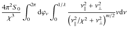
As an example, we consider an isotropic power-law dependence of the roughness power spectral density on the spatial frequency,
![]() (Church 1988). The integrals in Eqs. (22) and (23) then give, assuming
(Church 1988). The integrals in Eqs. (22) and (23) then give, assuming ![]() ,
,
![]() ,
and m<4,
,
and m<4,
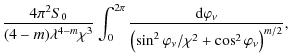
where we have used polar coordinates after the substitution
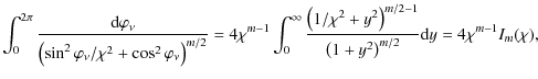
where
The scattering contribution is suppressed by a factor
where
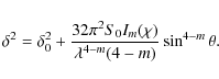
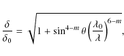
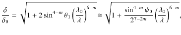
Equation (40) is now studied in more detail for a grazing-incidence mirror with one and two reflections, respectively. For a mirror with a single reflection and an object at infinity,
![]() ,
where
,
where ![]() is the angle of the principal ray at the focal plane with respect to the optical axis. Assuming that
is the angle of the principal ray at the focal plane with respect to the optical axis. Assuming that ![]() is small, Eq. (40) gives
is small, Eq. (40) gives
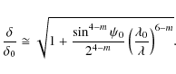
The ratio
where again
![\begin{figure}
\par\includegraphics[width=8.5cm,clip]{1506Fig2.ps}
\end{figure}](/articles/aa/full_html/2009/19/aa11506-08/img219.png) |
Figure 2:
Normalized beam width as a function of the normalized wavelength
for a single reflection optics with |
| Open with DEXTER | |
![\begin{figure}
\par\includegraphics[width=8.5cm,clip]{1506Fig3.ps}
\end{figure}](/articles/aa/full_html/2009/19/aa11506-08/img220.png) |
Figure 3:
Normalized beam width as a function of the normalized wavelength for a
two reflections optics with |
| Open with DEXTER | |
5 Conclusions
In the framework of the scalar theory of Fourier diffraction, we have derived the width of the angle spread function of a grazing-incidence optical system with cylindrical symmetry in the presence of roughness scattering. The derivation does not introduce further approximations in the theory except for assuming that the angle between the axial profile of the optics and the optical axis is small. Consequently, the results presented in this paper are more relevant to X-ray astronomy than other applications, such as EUV microlithography, that also use grazing-incidence mirrors with cylindrical symmetry but are characterized by quite large angles between the mirror profile and the optical axis.
When the small roughness approximation is applicable, the angle spread function itself can be expressed in a standard form as the convolution of the angle spread function of a perfectly smooth optics with an effective power spectral density related to the true power spectral density of surface roughness by line integration along an ellipse. This approximate expression for the angle spread function provides the correct expression for the width of the reflected and scattered beam and can be used for more accurate analyses of the scattering effects in X-ray telescopes. For example, it can be used to determine the encircled energy in the focal plane as a function of the encircling angular diameter.
Appendix A: Calculation of

We first show that the gradient of
![]() vanishes at the origin. We work in polar coordinates for
vanishes at the origin. We work in polar coordinates for ![]() ,
a vector of modulus f and anomaly
,
a vector of modulus f and anomaly
![]() .
Since the optical transfer function, Eq. (16), has cylindrical symmetry and thus is independent of
.
Since the optical transfer function, Eq. (16), has cylindrical symmetry and thus is independent of
![]() ,
we can simply ignore
,
we can simply ignore
![]() and just set
and just set
![]() .
The gradient of
.
The gradient of
![]() is given by
is given by
where
where
Since
We next calculate the Laplacian of
![]() at the origin, again ignoring
at the origin, again ignoring
![]() .
Using Eq. (A.1), we find that
.
Using Eq. (A.1), we find that
When we evaluate the above expression at the origin, the first two terms in the second line vanish because of the above argument about the value of the gradient of
To calculate the right-hand side of Eq. (A.3), we use Eqs. (17) and (18) and we obtain
Evaluating these expressions at f=0 gives
When Eqs. (A.4) and (A.5) are inserted back into Eq. (A.3), we obtain
which is Eq. (20) in the text.
Appendix B: Validity of the shadowing effects approximation
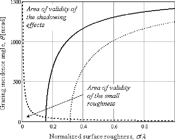 |
Figure B.1: Limit of validity of the multiple scattering and shadowing effects approximation (solid trace) and of the small roughness approximation (dashed trace). A relaxed limit of validity of the approximation is also plotted (dotted trace). |
| Open with DEXTER | |
The theory that leads to Eq. (6) and on which the present paper is based, requires, to remain valid, some assumptions about the properties of the optical system under consideration and the statistical properties of surface roughness. These assumptions, which are listed in Sect. 2, include the requirement that multiple reflections and shadowing effects can be ignored. In this Appendix, some considerations are discussed about the range of validity of this assumption and its relation to the small roughness approximation.
We can assume that multiple reflections and shadowing effects can be neglected if the grazing-incidence angle ![]() is larger than the rms slope error
is larger than the rms slope error ![]() in the direction of the optical axis, or
in the direction of the optical axis, or
Since
where

The limiting curve
It must be remarked that the above discussion is not limited to the analysis of the validity of the results presented in this paper but is applicable to the entire theory of the Fourier optics treatment of scattering from rough surfaces. Below
![]() ,
the theory is always applicable, irrespective of the value of the incident angle. Above
,
the theory is always applicable, irrespective of the value of the incident angle. Above ![]() /
/
![]() ,
instead, the grazing-incidence angle above which the theory is valid increases rapidly with
,
instead, the grazing-incidence angle above which the theory is valid increases rapidly with ![]() /
/![]() .
In particular, for grazing-incidence optics, the theory is not applicable even if the small roughness approximation holds. However, condition (B.3) is quite pessimistic because of the inequality sign in Eq. (B.2). Condition (B.3) also follows from Eq. (B.1) in the case of a single sinusoidal wave with rms value
.
In particular, for grazing-incidence optics, the theory is not applicable even if the small roughness approximation holds. However, condition (B.3) is quite pessimistic because of the inequality sign in Eq. (B.2). Condition (B.3) also follows from Eq. (B.1) in the case of a single sinusoidal wave with rms value ![]() and spatial frequency
and spatial frequency
![]() /
/![]() .
If a less restricting value of
.
If a less restricting value of
![]() is used in Eq. (B.2), the limiting curve for the application of the theory shifts to higher values of the ratio
is used in Eq. (B.2), the limiting curve for the application of the theory shifts to higher values of the ratio ![]() /
/![]() .
As an example, the curve obtained by substituting
.
As an example, the curve obtained by substituting
![]() with
with
![]() into Eq. (B.2) is also plotted in Fig. B.1 (dotted trace).
into Eq. (B.2) is also plotted in Fig. B.1 (dotted trace).
References
- Abbe, E. 1873, Archiv für Mikroskopische Anatomie, 9, 413 [CrossRef]
- Aschenbach, B. 1988, Appl. Opt., 27, 1404 [NASA ADS] [CrossRef]
- Bakshi, V., ed. 2008, EUV Lithography (Bellingham, WA: SPIE)
- Barbee, T. 1986, Opt. Eng., 25, 898
- Bookbinder, J., Smith, R., Hornschemeier, A., et al. 2008, in Proc. SPIE, 7011, 701102
- Born, M., & Wolf, E. 1980, Principles of Optics (Oxford, UK: Pergamon Press)
- Braat, J. 1997, in Proc. SPIE, 3190, 59
- Chase, R., & Speybroeck, L. V. 1973, Appl. Opt., 12, 1042 [NASA ADS] [CrossRef]
- Christensen, F., Hornstrup, A., & Schnopper, H. 1988, Appl. Opt., 27, 1548 [NASA ADS] [CrossRef]
- Church, E. 1988, Appl. Opt., 27, 1518 [NASA ADS] [CrossRef] (In the text)
- Church, E., & Takacs, P. 1993, Appl. Opt., 32, 3344 [NASA ADS] [CrossRef]
- Church, E., & Takacs, P. 1995, Opt. Eng., 34, 353 [NASA ADS] [CrossRef]
- Citterio, O., Bonelli, G., Conti, G., et al. 1988, Appl. Opt., 27, 1470 [NASA ADS] [CrossRef]
- Foltyn, T., Bergmann, K., Braun, S., et al. 2004, in Proc. SPIE, 5533, 37
- Friedrich, P., Bräuninger, H., Budau, B., et al. 2008, in Proc. SPIE, 7011, 70112T
- Gaskill, J. 1978, Linear Systems, Fourier Transforms, and Optics (New York, NY: Wiley)
- Gehrels, N., Chincarini, G., Giommi, P., et al. 2004, ApJ, 611, 1005 [NASA ADS] [CrossRef]
- Giacconi, R., Reidy, W., Vaiana, G., VanSpeybroeck, L., & Zehnpfennig, T. 1969, Space Sci. Rev., 9, 3 [NASA ADS] [CrossRef]
- Gondoin, P., de Chambure, D., Katwijk, K. V., et al. 1994, in Proc. SPIE, 2279, 86
- Goodman, J. 1968, Introduction to Fourier Optics (New York, NY: McGraw Hill)
- Harvey, J. 1995a, Appl. Opt., 34, 3715 [NASA ADS] [CrossRef]
- Harvey, J. 1995b, in Proc. SPIE, 2515, 246
- Harvey, J., Moran, E., & Zmek, W. 1988, Appl. Opt., 27, 1527 [NASA ADS] [CrossRef]
- Harvey, J., Lewotsky, K., & Thompson, A. 1996, Opt. Eng., 35, 2423 [NASA ADS] [CrossRef]
- Joensen, K., Voutov, P., Szentgyorgyi, A., et al. 1995, Appl. Opt., 34, 7935 [NASA ADS] [CrossRef]
- Karabacak, T., Zhao, Y., Stowe, M., et al. 2000, Appl. Opt., 39, 4658 [NASA ADS] [CrossRef]
- Papoulis, A. 1965, Probability, Random Variables, and Stochastic Processes (New York, NY: McGraw Hill) (In the text)
- Pareschi, G., & Ferrando, P. 2005, Exp. Astr., 20, 139 [NASA ADS] [CrossRef]
- Schellenberg, F., ed. 2008, Proc. SPIE: Emerging Lithographic Technologies XII, 6921
- Schäfer, D., Nisius, T., Früke, R., et al. 2006, in Proc. SPIE, 6317, 631704
- Silk, J. 1980, Annuals N.Y. Academy Sciences, 342, 116 [NASA ADS] [CrossRef]
- Smith, F. 1963, Appl. Opt., 2, 335 [NASA ADS] [CrossRef]
- Spiga, D. 2007, A&A, 468, 775 [NASA ADS] [CrossRef] [EDP Sciences] (In the text)
- Spiller, E. 1994, Soft X-ray Optics (Bellingham, WA: SPIE)
- Spiller, E. 2003, in Proc. SPIE, 5193, 89
- Stearns, D., Gaines, D., Sweeney, D., & Gullikson, E. 1998, J. Appl. Phys., 84, 1003 [NASA ADS] [CrossRef]
- Watson, G. 1966, A Treatise on the Theory of Bessel Functions, 2nd edn. (Cambridge, UK: Cambridge University Press) (In the text)
- Weisskopf, M., Tananbaum, H., Speybroeck, L. V., & O'Dell, S. 2000, in Proc. SPIE, 4012, 2
- Wolter, H. 1952a, Ann. Phys., 10, 286 [CrossRef]
- Wolter, H. 1952b, Ann. Phys., 10, 94 [CrossRef] (In the text)
- Yamashita, K., Kuneida, H., Tawara, Y., et al. 1999, in Proc. SPIE, 3766, 327
- Zhao, P., & Spreybroeck, L. V. 2003, in Proc. SPIE, 4851, 124
- Zocchi, F. 2009, Appl. Opt., 48, 436 [NASA ADS] [CrossRef] (In the text)
- Zocchi, F., & Vernani, D. 2007, in Proc. SPIE, 6688, 66880B
All Figures
| |
Figure 1: Geometry of the grazing-incidence optics with cylindrical symmetry: conceptual 3D drawing ( left) anf optics cross section ( right). |
| Open with DEXTER | |
| In the text | |
| |
Figure 2:
Normalized beam width as a function of the normalized wavelength
for a single reflection optics with |
| Open with DEXTER | |
| In the text | |
| |
Figure 3:
Normalized beam width as a function of the normalized wavelength for a
two reflections optics with |
| Open with DEXTER | |
| In the text | |
| |
Figure B.1: Limit of validity of the multiple scattering and shadowing effects approximation (solid trace) and of the small roughness approximation (dashed trace). A relaxed limit of validity of the approximation is also plotted (dotted trace). |
| Open with DEXTER | |
| In the text | |
Copyright ESO 2009
Current usage metrics show cumulative count of Article Views (full-text article views including HTML views, PDF and ePub downloads, according to the available data) and Abstracts Views on Vision4Press platform.
Data correspond to usage on the plateform after 2015. The current usage metrics is available 48-96 hours after online publication and is updated daily on week days.
Initial download of the metrics may take a while.