| Issue |
A&A
Volume 498, Number 3, May II 2009
|
|
|---|---|---|
| Page(s) | 987 - 992 | |
| Section | Numerical methods and codes | |
| DOI | https://doi.org/10.1051/0004-6361/200911681 | |
| Published online | 19 March 2009 | |
A 3D radiative transfer framework
V. Homologous flows
E. Baron1,2,3 - P. H. Hauschildt1 - B. Chen2
1 - Hamburger Sternwarte, Gojenbergsweg 112, 21029 Hamburg, Germany
2 - Homer L. Dodge Department of Physics and Astronomy, University of Oklahoma, 440 W Brooks, Rm 100, Norman, OK 73019-2061 USA
3 - Computational Research Division, Lawrence Berkeley National Laboratory, MS 50F-1650, 1 Cyclotron Rd, Berkeley, CA 94720 USA
Received 19 January 2009 / Accepted 6 March 2009
Abstract
Context. Observations and theoretical calculations have shown the importance of non-spherically symmetric structures in supernovae. Thus, the interpretation of observed supernova spectra requires the ability to solve the transfer equation in 3-D moving atmospheres.
Aims. We present an implementation of the solution of the radiative transfer equation in 3-D homologously expanding atmospheres in spherical coordinates. The implementation is exact to all orders in v/c.
Methods. We use the methods that we have developed in previous papers in this series as well as a new affine method that makes use of the fact that photons travel on straight lines. The affine method greatly facilitates delineating the characteristics and can be used in the case of strong-gravitational and arbitrary-velocity fields.
Results. We compare our results in 3-D for spherically symmetric test problems with high velocity fields (up to 87% of the speed of light) and find excellent agreement, when the number of momentum space angles is high. Our well-tested 1-D results are based on methods where the momentum directions vary along the characteristic (co-moving momentum directions). Thus, we are able to verify both the analytic framework and its numerical implementation. Additionally, we have been able to test the parallelization over characteristics. Using 5122 momentum angles we ran the code on 16 384 Opteron processors and achieved excellent scaling.
Conclusions. It is now possible to calculate synthetic spectra from realistic 3D hydro simulations. This should open an era of progress in hydro modeling, similar to that that occurred in the 1980s when 1-D models were confronted with synthetic spectra.
Key words: radiative transfer - relativity - stars: supernovae: general
1 Introduction
Supernovae of all types are known to deviate significantly from
spherical symmetry. The evidence comes from both flux spectra, but
particularly from the interpretation of spectropolarimetry
(see Wang & Wheeler 2008, and references therein). In the case of
core-collapse supernovae, the asymmetry is thought to be due to the
underlying central engine which is probably asymmetric and this leads
to geometrically asymmetric ejecta, with the asymmetry growing as one
gets closer to the central engine (thus ``stripped'' supernovae such
as type Ic are significantly more asymmetric than supernovae with
intact hydrogen envelopes such as type IIP). Type Ia (thermonuclear)
supernovae are thought to be geometrically rather round but the
composition is thought to be asymmetrical. Since the light curve of
type Ia supernovae is powered by the radioactive decay of
![]() and its
products, asymmetries in the
and its
products, asymmetries in the
![]() distribution will lead to asymmetries
in the ionization fractions and opacities that will produce
polarization and alter the flux spectra. Thus, particularly in type Ia
supernovae one can accurately calculate light curves and spectra
assuming homologous flow (
distribution will lead to asymmetries
in the ionization fractions and opacities that will produce
polarization and alter the flux spectra. Thus, particularly in type Ia
supernovae one can accurately calculate light curves and spectra
assuming homologous flow (
![]() )
but including the
geometrical or compositional asymmetry in three dimensions.
)
but including the
geometrical or compositional asymmetry in three dimensions.
In this series of papers (Baron & Hauschildt 2007; Hauschildt & Baron 2009,2008,2006, henceforth Papers I-IV) we have built up the full characteristics method of solving the transfer equation in 3-D for static atmospheres in a variety of geometries. Here we build on the results of Paper IV for spherical geometry as well as those of Chen et al. (2007) for the affine method.
2 Transfer equation
Chen et al. (2007) showed that the transfer equation in flat spacetime could be written in terms of an affine parameter and that the right hand side could be evaluated in the co-moving frame provided that the wavelength (or frequency) was evaluated in the co-moving frame. However, the momentum directions could be held constant and coincide with those of the observer's frame.
We define the rest frame photon direction in spherical coordinates as
| (1) |
or in Cartesian coordinates
| (2) |
and the starting position of the photon
| (3) |
The 3-D geodesic can be parametrized as
where s is the rest frame physical distance related to the affine parameter

and is measured starting from
 |
(6) |
 |
(7) |
and
 |
(8) |
where
| |
= | ||
| = | x0px+y0py+z0pz. | (9) |
Note also that
 |
(10) |
From Eqs. (5) above and (18) of Chen et al. (2007), we find
with
![\begin{displaymath}
\frac{\lambda_\infty}{\lambda}=\gamma(r)\left[1-\dot{r}\beta(r)\right]\equiv
f(s).
\end{displaymath}](/articles/aa/full_html/2009/18/aa11681-09/img24.png)
From Eq. (12) we find

Now we have
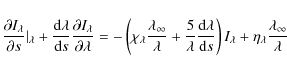
![\begin{displaymath}\frac{\partial I_\lambda}{\partial s}\vert _\lambda + a(s)\la...
...ambda}=-[\chi_\lambda f(s)+5 a(s)]I_\lambda+\eta_\lambda f(s).
\end{displaymath}](/articles/aa/full_html/2009/18/aa11681-09/img28.png) |
(14) |
Finally, this can be put into the standard form used in PHOENIX (Hauschildt & Baron 2004b,1999)
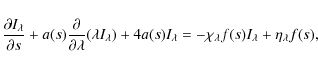
where a(s) is given by Eq. (13), and f(s) is given by Eq. (12).
In order to finite difference this equation we need to explicitly
difference the
![]() term. As described in Chen et al. (2007) we can write
term. As described in Chen et al. (2007) we can write
 |
(16) |
Then, Eq. (15) can be written as:
Now we can define an effective optical depth,
| |
= |  |
(18) |
| (19) |
which defines

which defines
The more sophisticated discretization in ![]() described in Hauschildt & Baron (2004a) or Knop et al. (2009) can also be implemented. For the case of arbitrary velocity fields the method of Knop et al. (2009) will be
required. Nevertheless, this straightforward method yields excellent results when compared with the more sophisticated treatment used in the 1-D code (see below).
described in Hauschildt & Baron (2004a) or Knop et al. (2009) can also be implemented. For the case of arbitrary velocity fields the method of Knop et al. (2009) will be
required. Nevertheless, this straightforward method yields excellent results when compared with the more sophisticated treatment used in the 1-D code (see below).
3 Angular integration
To solve the scattering problem in the co-moving frame, we need to calculate the mean intensity and
![]() in the co-moving frame. Recall that the specific intensity is calculated in a frame
where five of the six phase-space variables are actually observer's frame quantities. In particular, the two momentum directions are fixed observer's frame quantities. Thus, we need to perform the angular integration in the co-moving frame. We have
in the co-moving frame. Recall that the specific intensity is calculated in a frame
where five of the six phase-space variables are actually observer's frame quantities. In particular, the two momentum directions are fixed observer's frame quantities. Thus, we need to perform the angular integration in the co-moving frame. We have
| (22) |
and
![\begin{displaymath}p = \frac{hc}{\lambda}[1,\vec{\hat n}]
.\end{displaymath}](/articles/aa/full_html/2009/18/aa11681-09/img45.png) |
(23) |
Then

Now
![\begin{displaymath}u\cdot p = \frac{hc}{\lambda}\gamma [ 1 - \vec{\beta\cdot
\hat n}],\>\>\> u_0\cdot p = \frac{hc}{\lambda}\cdot
\end{displaymath}](/articles/aa/full_html/2009/18/aa11681-09/img47.png) |
(24) |
Thus
3.0.1 Computation of

The computation of
![]() proceeds following the same procedure as
in Paper I. As demonstrated by Olson et al. (1986) and Olson & Kunasz (1987), the
coefficients
proceeds following the same procedure as
in Paper I. As demonstrated by Olson et al. (1986) and Olson & Kunasz (1987), the
coefficients ![]() ,
,
![]() ,
and
,
and ![]() can be used to construct diagonal and tri-diagonal
can be used to construct diagonal and tri-diagonal
![]() operators for 1D radiation transport problems. In fact, up to the full
operators for 1D radiation transport problems. In fact, up to the full
![]() matrix can be constructed by a straightforward extension of the idea
(Hauschildt & Baron 2004a; Hauschildt et al. 1994). These non-local
matrix can be constructed by a straightforward extension of the idea
(Hauschildt & Baron 2004a; Hauschildt et al. 1994). These non-local
![]() operators not only lead to
excellent convergence rates but they avoid the problem of false
convergence that is inherent in the
operators not only lead to
excellent convergence rates but they avoid the problem of false
convergence that is inherent in the ![]() iteration method and can also be
an issue for diagonal (purely local)
iteration method and can also be
an issue for diagonal (purely local)
![]() operators. Therefore, it is
highly desirable to implement a non-local
operators. Therefore, it is
highly desirable to implement a non-local
![]() for the 3D case. The
tri-diagonal operator in the 1D case is simply a nearest neighbor
for the 3D case. The
tri-diagonal operator in the 1D case is simply a nearest neighbor
![]() that
considers the interaction of a point with its two direct neighbors. In the 3D
case, the nearest neighbor
that
considers the interaction of a point with its two direct neighbors. In the 3D
case, the nearest neighbor
![]() considers the interaction of a voxel with
the (up to) 33-1=26 surrounding voxels (this definition considers a
somewhat larger
range of voxels than a strictly face-centered view of just 6 nearest neighbors).
This means that the non-local
considers the interaction of a voxel with
the (up to) 33-1=26 surrounding voxels (this definition considers a
somewhat larger
range of voxels than a strictly face-centered view of just 6 nearest neighbors).
This means that the non-local
![]() requires the storage of 27
(26 surrounding voxels plus local, i.e., diagonal effects) times the total
number of voxels
requires the storage of 27
(26 surrounding voxels plus local, i.e., diagonal effects) times the total
number of voxels
![]() elements.
elements.
The construction of the
![]() operator proceeds in the same way as
discussed in Hauschildt (1992) and Paper I. In the 3D case, the
``previous'' and ``next'' voxels along each characteristic must be known so that
the contributions can be attributed to the correct voxel. Therefore, we use a
data structure that attaches to each voxel its effects on its neighbors.
The scheme can be extended trivially to include longer range interactions
for better convergence rates (in particular on larger voxel grids). However,
the memory requirements to simply store
operator proceeds in the same way as
discussed in Hauschildt (1992) and Paper I. In the 3D case, the
``previous'' and ``next'' voxels along each characteristic must be known so that
the contributions can be attributed to the correct voxel. Therefore, we use a
data structure that attaches to each voxel its effects on its neighbors.
The scheme can be extended trivially to include longer range interactions
for better convergence rates (in particular on larger voxel grids). However,
the memory requirements to simply store
![]() ultimately scales like
n3 where n is the total number of voxels. The storage requirements can be
reduced by, e.g., using
ultimately scales like
n3 where n is the total number of voxels. The storage requirements can be
reduced by, e.g., using
![]() 's of different widths for different voxels.
Storage requirements are not so much a problem if a domain decomposition
parallelization method is used and enough processors are available.
's of different widths for different voxels.
Storage requirements are not so much a problem if a domain decomposition
parallelization method is used and enough processors are available.
We describe here the general procedure of calculating the
![]() with arbitrary bandwidth, up to the full
with arbitrary bandwidth, up to the full ![]() -operator, for the method in
spherical symmetry (Hauschildt et al. 1994). The construction of the
-operator, for the method in
spherical symmetry (Hauschildt et al. 1994). The construction of the
![]() is
described in Olson & Kunasz (1987), so that we here summarize the relevant
formulae. In the method of Olson & Kunasz (1987), the elements of the row of
is
described in Olson & Kunasz (1987), so that we here summarize the relevant
formulae. In the method of Olson & Kunasz (1987), the elements of the row of
![]() are
computed by setting the incident intensities (boundary conditions) to zero and setting
S(ix,iy,iz)=1 for one voxel
(ix,iy,iz) and performing a formal
solution analytically.
are
computed by setting the incident intensities (boundary conditions) to zero and setting
S(ix,iy,iz)=1 for one voxel
(ix,iy,iz) and performing a formal
solution analytically.
We describe the construction of
![]() using the example of a single characteristic. The contributions to the
using the example of a single characteristic. The contributions to the
![]() at a voxel j are given by
at a voxel j are given by
These contributions are computed along a characteristic, here i labels the voxels along the characteristic under consideration. These contributions are integrated over solid angle with the same method (either deterministic or through Monte-Carlo integration) that is used for the computation of J. For a nearest neighbor
4 From co-moving frame to global inertial frame
The specific intensity ![]() is observer dependent, it is related to the observer invariant phase space distribution F(x,p) by
is observer dependent, it is related to the observer invariant phase space distribution F(x,p) by
 |
(31) |
therefore, the invariant quantity should be
 |
(32) |
We do not need to transform the direction vector, because when we write down our transfer equation, the only co-moving quantity we used is the co-moving wavelength, the other two momentum space variables (e.g., nx, ny) are global inertial (for the case we are working on, the
5 Application examples
As a first step we have built upon the MPI parallelized Fortran 95 program described in Papers I-IV. The parallelization of the formal solution is presently implemented over solid angle space as this is the simplest parallelization option and also one of the most efficient (a domain decomposition parallelization method will be discussed in a subsequent paper). In addition, the Jordan solver of the Operator splitting equations is parallelized with MPI. The number of parallelization related statements in the code is small.
Our basic continuum scattering test problem is similar to that discussed in
Hauschildt (1992), Hauschildt & Baron (2004a) and Papers I-II. This test problem covers a
large dynamic range of about 9 dex in the opacities and overall optical depth
steps along the characteristics and, in our experience, constitutes a reasonably challenging setup for the radiative transfer code. The application of the 3D code to ``real'' problems is in preparation and requires a substantial amount of development work (in progress).
Comparing this test case to real world problems in 1D we have found that this test is close to the worst case scenario and that convergence, etc is generally better in real world problems. We use a
sphere with a grey continuum opacity parametrized by a power law in the continuum optical
depth
![]() .
The basic model parameters are:
.
The basic model parameters are:
- 1.
- Inner radius
 cm, outer radius
 cm.
cm.
- 2.
- Minimum optical depth in the continuum
 and maximum optical depth in the continuum
 .
.
- 3.
- Grey temperature structure with
 K.
K.
- 4.
- Outer boundary condition
 and diffusion inner boundary condition for all wavelengths.
- 5.
- Continuum extinction
 ,
with the constant C fixed by the radius and optical depth grids.
,
with the constant C fixed by the radius and optical depth grids.
- 6.
- Parametrized coherent and isotropic continuum scattering by defining
(33)
with .
.
 and
and
 are the continuum absorption and scattering coefficients.
![\begin{figure}
\par\includegraphics[angle=90,width=8.5cm,clip]{1681fig1.eps}
\end{figure}](/articles/aa/full_html/2009/18/aa11681-09/img86.png) |
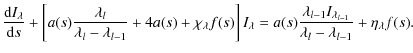
Figure 1:
The results of 1-D calculations are compared with 3-D calculations for
|
| Open with DEXTER | |
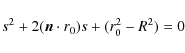
5.1 LTE tests
In this test we have set
![]() to test the accuracy of the formal solution by comparing to the results of the 1D code. The 1D solver uses 64 radial points, distributed logarithmically in optical depth. For the 3D solver we tested `moderate' grids with
to test the accuracy of the formal solution by comparing to the results of the 1D code. The 1D solver uses 64 radial points, distributed logarithmically in optical depth. For the 3D solver we tested `moderate' grids with
![]() and
and
![]() points along each axis, for a total of
points along each axis, for a total of
![]() voxels.
The momentum space discretization uses in general,
voxels.
The momentum space discretization uses in general,
![]() points. In
Fig. 1 we show the mean intensities as a function of
distance from the center for both the 1D (+ symbols) and the 3D solver. For the 3D results J is plotted at every voxel on the surface and the spherical symmetry is reproduced very well at every
point on the surface. The results show excellent agreement between the two solutions, thus the
3D RT formal solution is comparable in accuracy to the 1D formal solution. Figure 1 shows the results for four different maximum velocities, and clearly indicates that the 3D RT solution is just as accurate as the 1D code. This is actually quite a
nice demonstration since the affine method used in the 3D code is completely different from the full co-moving momentum space method used in the 1-D code, that is, the specific intensity is solved for in different frames in the two codes. However, since J depends
only on the co-moving frequency they can be directly compared in the same frame.
points. In
Fig. 1 we show the mean intensities as a function of
distance from the center for both the 1D (+ symbols) and the 3D solver. For the 3D results J is plotted at every voxel on the surface and the spherical symmetry is reproduced very well at every
point on the surface. The results show excellent agreement between the two solutions, thus the
3D RT formal solution is comparable in accuracy to the 1D formal solution. Figure 1 shows the results for four different maximum velocities, and clearly indicates that the 3D RT solution is just as accurate as the 1D code. This is actually quite a
nice demonstration since the affine method used in the 3D code is completely different from the full co-moving momentum space method used in the 1-D code, that is, the specific intensity is solved for in different frames in the two codes. However, since J depends
only on the co-moving frequency they can be directly compared in the same frame.
As shown in Paper I, for the conditions used in these tests a larger number of solid angle points significantly improves the accuracy of the mean intensities. Our tests show that reasonable accuracy can be achieved with as few as 162 momentum space points, but in these test calculations we have used more points in order to really compare the 3D results to the 1D results. A full investigation of the number of angle points needed for realistic asymmetric calculations will be the subject of future work.
The line of the simple 2-level model atom is parametrized by the ratio of the profile averaged line opacity ![]() to the continuum opacity
to the continuum opacity
![]() and the line thermalization parameter
and the line thermalization parameter
![]() .
For the test cases presented below, we have used
.
For the test cases presented below, we have used
![]() and a constant temperature and thus a constant thermal part of the source function for simplicity (and to save computing time) and set
and a constant temperature and thus a constant thermal part of the source function for simplicity (and to save computing time) and set
![]() to simulate a strong line, with
to simulate a strong line, with
![]() (see below). With this setup, the optical depths as seen in the line range from 10-2 to 106. We use 92 wavelength points to model the full line profile, including wavelengths outside the line for the continuum. We did not require the line to thermalize at the center of the test configurations, this is a typical situation one encounters in a full 3D configurations as the location (or even existence) of the thermalization depths becomes more ambiguous than in the 1D case.
(see below). With this setup, the optical depths as seen in the line range from 10-2 to 106. We use 92 wavelength points to model the full line profile, including wavelengths outside the line for the continuum. We did not require the line to thermalize at the center of the test configurations, this is a typical situation one encounters in a full 3D configurations as the location (or even existence) of the thermalization depths becomes more ambiguous than in the 1D case.
The sphere is put at the center of the Cartesian grid, which is in each axis 10% larger than the radius of the sphere. For the test calculations we use voxel grids with the same
number of spatial points in each direction (see below). The solid angle space was discretized in
![]() with
with
![]() Unless otherwise stated, the tests were run on parallel computers using a variety of number of CPUs, architectures, and interconnects.
Unless otherwise stated, the tests were run on parallel computers using a variety of number of CPUs, architectures, and interconnects.
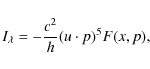
![\begin{figure}
\par\includegraphics[angle=90,width=8cm,clip]{1681fig2.eps}
\end{figure}](/articles/aa/full_html/2009/18/aa11681-09/img98.png) |
Figure 2:
The results of 1-D calculations for a scattering line are compared with 3-D calculations for
|
| Open with DEXTER | |
5.2 LTE line and continuum test
We first have set
![]() to test the accuracy of the formal solution by comparing to the results of the 1D code. The 1D solver uses 64 radial points, distributed logarithmically in optical depth. Comparing the line mean intensities
to test the accuracy of the formal solution by comparing to the results of the 1D code. The 1D solver uses 64 radial points, distributed logarithmically in optical depth. Comparing the line mean intensities ![]() as function of distance from the center for both the 1D and the 3D solver we again found excellent agreement.
as function of distance from the center for both the 1D and the 3D solver we again found excellent agreement.
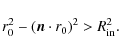
5.3 Tests with line scattering
We have run a number of test calculations similar to the LTE case but with line
scattering included. In Fig. 2 we show the co-moving ![]() as a function of
as a function of ![]() for
for
![]() with
with
![]() and
and
![]() .
The 3D calculations compare very well to the 1D calculations. The small variation in some parts of the surface of the sphere (each black line represents a pixel on the
surface of the sphere) is due to the different wavelength discretization. The 3D case uses only the simple method described above, whereas the 1D case uses the full Crank-Nicholson-like method
described in Hauschildt & Baron (2004a).
.
The 3D calculations compare very well to the 1D calculations. The small variation in some parts of the surface of the sphere (each black line represents a pixel on the
surface of the sphere) is due to the different wavelength discretization. The 3D case uses only the simple method described above, whereas the 1D case uses the full Crank-Nicholson-like method
described in Hauschildt & Baron (2004a).
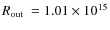
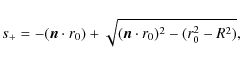
Figure 3 shows the wall-clock time as a function of
resolution (number of momentum-space angles ![]() and
and ![]() or
number of CPUs). The computational work is kept constant with each CPU
required to calculate 16 characteristics. The modest (14%) increase
in wall-clock time from 16 CPUs to 16 384 CPUs is acceptable given the
huge increase in communication required and the fact that load
balancing is quite simple. The wall-clock time for this test was about
625 s for each direction angle. The memory usage is controlled by the
size of the spatial grid (this is also true in Papers I-IV). The only
additional storage is that the values of the intensity for both the
previous and current wavelength point must be stored. The total memory per
process was about 100 MB.
or
number of CPUs). The computational work is kept constant with each CPU
required to calculate 16 characteristics. The modest (14%) increase
in wall-clock time from 16 CPUs to 16 384 CPUs is acceptable given the
huge increase in communication required and the fact that load
balancing is quite simple. The wall-clock time for this test was about
625 s for each direction angle. The memory usage is controlled by the
size of the spatial grid (this is also true in Papers I-IV). The only
additional storage is that the values of the intensity for both the
previous and current wavelength point must be stored. The total memory per
process was about 100 MB.
![\begin{figure}
\par\includegraphics[angle=90,width=8.5cm,clip]{1681fig3.eps}
\end{figure}](/articles/aa/full_html/2009/18/aa11681-09/img105.png) |
Figure 3:
The wall-clock time to solve a scattering line
|
| Open with DEXTER | |
6 Wavelength parallelization
We have implemented and tested a ``pipeline'' wavelength parallelization method using wavelength clusters in the manner described in Baron & Hauschildt (1998). As in Baron & Hauschildt (1998), the parallelization over characteristics is done within a ``wavelength cluster'' and each worker thus must send only its values of the specific intensity to the corresponding process in the next wavelength cluster. For the simple test problems considered so far the opacity calculation is trivial and hence, there is no speedup (but also no penalty) for this wavelength parallelization. However, in real world problems the time to calculate the opacities is roughly equal to the time required to solve the transfer equation and this leads to linear speedups in the 1D case of up to about a factor of eight.
7 Conclusions
We have implemented the affine method described in Chen et al. (2007) for the case of homologous flows and shown that it gives excellent results compared to the full co-moving method that we use in our 1D code. We have also been able to parallelize it both over characteristic and wavelength. The characteristic scaling is excellent and immediately brings us into the forefront of massively parallel computation. The next step is to include the 3D calculations in the full real world code and begin applying it to numerous astrophysical problems.
Acknowledgements
This work was supported in part by SFB 676 from the DFG, NASA grant NAG5-12127, NSF grant AST-0707704, and US DOE Grant DE-FG02-07ER41517. This research used resources of the National Energy Research Scientific Computing Center (NERSC), which is supported by the Office of Science of the US Department of Energy under Contract No. DE-AC02-05CH11231; and the Höchstleistungs Rechenzentrum Nord (HLRN). We thank all these institutions for a generous allocation of computer time.
Appendix A: Determining s from Coordinates
The characteristics are followed through the voxel grid from an
entry boundary point to an exit boundary point. It is convenient
to choose some particular voxel as a ``starting point'' r0 and determine
the distance s to the two boundary points. We will choose our sign
convention such that the distance to the entry point is negative and the distance to
the exit point is positive. Given a starting point r0 we can find the distance to a boundary
point R (where
![]() ,
or
,
or
![]() )
from
Eq. (4) and find
)
from
Eq. (4) and find
The characteristics can be divided into three classes. Tangential characteristics (those that do not hit the inner boundary Rin have
and satisfy the constraint that the impact parameter is greater than
 |
(A.2) |
For this case, Eq. (A.1) has two solutions
 |
(A.3) |
and
 |
(A.4) |
such that
| (A.5) |
Core-intersecting characteristics include two cases, incoming and outgoing rays. Incoming core-intersecting characteristics are determined by
| (A.6) |
where
and there is only one solution
 |
(A.7) |
the other solution
 |
(A.8) |
should be dropped because it passes through the core. Here
| s-<0<s+. | (A.9) |
For outgoing core-intersecting characteristics
| (A.10) |
this time the characteristic should start from the core
For this case
 |
(A.11) |
is the desired solution and the other solution
 |
(A.12) |
passes through the core. In this case,
| 0>s->s+. | (A.13) |
References
All Figures
| |
Figure 1:
The results of 1-D calculations are compared with 3-D calculations for
|
| Open with DEXTER | |
| In the text | |
| |
Figure 2:
The results of 1-D calculations for a scattering line are compared with 3-D calculations for
|
| Open with DEXTER | |
| In the text | |
| |
Figure 3:
The wall-clock time to solve a scattering line
|
| Open with DEXTER | |
| In the text | |
Copyright ESO 2009
Current usage metrics show cumulative count of Article Views (full-text article views including HTML views, PDF and ePub downloads, according to the available data) and Abstracts Views on Vision4Press platform.
Data correspond to usage on the plateform after 2015. The current usage metrics is available 48-96 hours after online publication and is updated daily on week days.
Initial download of the metrics may take a while.