| Issue |
A&A
Volume 498, Number 3, May II 2009
|
|
|---|---|---|
| Page(s) | 885 - 889 | |
| Section | The Sun | |
| DOI | https://doi.org/10.1051/0004-6361/200811171 | |
| Published online | 19 March 2009 | |
Dynamics of coronal mass ejections in the interplanetary medium
A. Borgazzi1,2 - A. Lara2 - E. Echer1 - M. V. Alves1
1 - National Institute for Space Research, INPE, SP-Brazil
2 -
Instituto de Geofísica, Universidad Nacional Autónoma de
México, México
Received 16 October 2008 / Accepetd 13 February 2009
Abstract
Context. Coronal mass ejections (CMEs) are large plasma structures expelled from the low corona to the interplanetary space with a wide range of speeds. In the interplanetary medium CMEs suffer changes in their speeds because of interaction with the ambient solar wind.
Aims. To understand the interplanetary CME (ICME) dynamics, we analyze the interaction between these structures and the ambient solar wind (SW), approaching the problem from the hydrodynamic point of view.
Methods. We assume that the dynamics of the system is dominated by two kinds of drag-force dependence on speed (U), as ![]() and
and
![]() .
Furthermore, we propose a model that takes variations of the ICME radius (R) and SW density (
.
Furthermore, we propose a model that takes variations of the ICME radius (R) and SW density (
![]() )
into account as a function of the distance (x) as
R(x) = x0.78 and
)
into account as a function of the distance (x) as
R(x) = x0.78 and
![]() ,
respectively. Then, we solve the equation of motion and present exact solutions
,
respectively. Then, we solve the equation of motion and present exact solutions
Results. Considering CME speeds measured at a few solar radii and at one AU, we were able to constrain the values of the constants (viscosity and drag coefficient) for the linear (U) and quadratic (U2) speed dependences, which seems to reproduce the ICME - SW system well. We found different solutions in which the concavity of the curves of the ICME speed profile changes, depending on the dominant factor, either the ICME radius or the SW density.
Conclusions. This work shows that the macroscopic ICME propagation may be described by the hydrodynamic theory and that it is possible to find analytical solutions for the ICME-SW interaction.
Key words: hydrodynamics - Sun: coronal mass ejections (CMEs) - interplanetary medium
1 Introduction
A major solar transient event that injects large amounts
of mass and energy
to the interplanetary space is known as coronal mass ejection (CME).
These vast structures of plasma and magnetic field, observed principally
with white light coronographs, are known as the main link between the
Sun's activity and geomagnetic storms (Gosling et al. 1999).
We classify CMEs according to their initial speed into two categories:
``slow'' for CMEs with speed lower than
![]() ;
and ``fast'' for CMEs with speeds higher than
;
and ``fast'' for CMEs with speeds higher than
![]() .
In both cases, an interaction between the ICME structure (the remnant of a CME in the interplanetary medium) and the ambient solar wind takes place.
This interaction can be described as a momentum transfer involving two
systems, a body (the CME) moving in an ambient fluid, the solar wind (SW).
In the case of ``fast'' CMEs the process causes a deceleration of the ICME structure from its initial speed (in the range of
.
In both cases, an interaction between the ICME structure (the remnant of a CME in the interplanetary medium) and the ambient solar wind takes place.
This interaction can be described as a momentum transfer involving two
systems, a body (the CME) moving in an ambient fluid, the solar wind (SW).
In the case of ``fast'' CMEs the process causes a deceleration of the ICME structure from its initial speed (in the range of
![]() to
to
![]() )
towards the value of
the SW speed (
)
towards the value of
the SW speed (
![]() )
at distances of a few AU.
In general, the ICME dynamics have been deduced by complementary
observations (of the same event) close to the Sun by coronographs and close
to the Earth by satellite in-situ measurements.
This restriction (observations from only two points) has been overcome
by the interplanetary scintillation (IPS) technique (Manoharan 2006)
and direct white-light observations in the interplanetary medium
(Tappin 2004).
)
at distances of a few AU.
In general, the ICME dynamics have been deduced by complementary
observations (of the same event) close to the Sun by coronographs and close
to the Earth by satellite in-situ measurements.
This restriction (observations from only two points) has been overcome
by the interplanetary scintillation (IPS) technique (Manoharan 2006)
and direct white-light observations in the interplanetary medium
(Tappin 2004).
Using these observational methods, the acceleration
of ICMEs has been confirmed; however, the profile and mechanisms of the
ICME dynamics are still unknown.
Many efforts have been made to describe the dynamics of ICMEs.
Different kinds of theoretical, empirical, and numerical models have been
studied. Recent analytical models of ICME propagation have been presented
by Canto et al. (2005) and Borgazzi et al. (2008, hereafter Paper 1).
Canto et al. (2005) studied the dynamics of
a fluctuation in density and speed starting at the base of the solar
corona and traveling in the ambient solar wind. They used a kinematic approximation, proposed CME properties as velocity, density, and temperature,
and found the ICME travel time from a few solar radii (![]() )
to one AU.
In Paper 1, the authors found exact solutions for the behavior of the speed
versus time of ICMEs.
The interaction between the ICME and the surrounding medium is described by
the action of viscous forces, and values of drag and viscous coefficients for the medium were obtained.
Empirical models were developed mainly to forecast the 1 AU arrival time
of ICMEs (e.g. Gopalswamy et al. 2005,2000,2001).
The methodology applied in these works
consists on the establishment of relationships between the observed data,
i.e., the CME initial speed; speeds observed
in the interplanetary medium; and the mean acceleration acting on the ICMEs.
The studies reported by Vrsnak et al. (2004,2002,2007); Vrsnak (2001)
may be considered in the same branch, with the difference that
in these cases the studies are done, from the point of view of viscous
forces acting on the ICMEs.
The group of numerical simulation of the transport of ICMEs is more numerous
(e.g. Odstrcil et al. 1999b; Cargill et al. 1996; Gonzalez-Esparza et al. 2003; Odstrcil et al. 1999a; Vandas et al. 1995; Cargill 2004; Chen 1996).
They generally study the evolution, through the
interplanetary space, of some properties
(temperature, density and speed) of the plasma structure
(plasmoids or magnetic clouds).
)
to one AU.
In Paper 1, the authors found exact solutions for the behavior of the speed
versus time of ICMEs.
The interaction between the ICME and the surrounding medium is described by
the action of viscous forces, and values of drag and viscous coefficients for the medium were obtained.
Empirical models were developed mainly to forecast the 1 AU arrival time
of ICMEs (e.g. Gopalswamy et al. 2005,2000,2001).
The methodology applied in these works
consists on the establishment of relationships between the observed data,
i.e., the CME initial speed; speeds observed
in the interplanetary medium; and the mean acceleration acting on the ICMEs.
The studies reported by Vrsnak et al. (2004,2002,2007); Vrsnak (2001)
may be considered in the same branch, with the difference that
in these cases the studies are done, from the point of view of viscous
forces acting on the ICMEs.
The group of numerical simulation of the transport of ICMEs is more numerous
(e.g. Odstrcil et al. 1999b; Cargill et al. 1996; Gonzalez-Esparza et al. 2003; Odstrcil et al. 1999a; Vandas et al. 1995; Cargill 2004; Chen 1996).
They generally study the evolution, through the
interplanetary space, of some properties
(temperature, density and speed) of the plasma structure
(plasmoids or magnetic clouds).
To better understand the ICME behavior and to encourage this kind of work (from a theoretical point of view), in this work we approach the study of the ICMEs dynamics using the hydrodynamics theory and considering the ICME - SW system as two interacting fluids, under the action of viscous forces without taking the microscopic details of this interaction into account.
2 Dynamical propagation model of ICMEs
2.1 Initial ICME conditions
In this work we concentrate in the ICME dynamics, from ![]() 30 to
30 to
![]() 215
215 ![]() .
As the initial point is far enough from the solar surface,
we assume the following considerations, presented by Chen (1996) and Sheeley et al. (1997):
.
As the initial point is far enough from the solar surface,
we assume the following considerations, presented by Chen (1996) and Sheeley et al. (1997):
-
the gravity force is negligible. For example,
in Fig. 7 of Chen (1996) the gravity force tends to zero at
approximately 110 min after CME initiation, corresponding
to a distance of the expanding loop apex of
 2
2  (see Fig. 5
of the same paper);
(see Fig. 5
of the same paper);
-
the Lorentz force is negligible.
In Fig. 9 of Chen (1996),
the Lorentz force is practically zero after 200 min of the CME initiation. This time corresponds to an apex height
of 6 ;
-
the solar wind speed is constant.
At 30
the solar wind has already been formed. We assume a constant speed
of 400 km s-1. Observationally, Sheeley et al. (1997) found that this constant
speed begins at approximately 30 .
Some models assume a speed profile
of the form
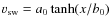 and adjust the constants a0 and b0to obtain a constant speed (400 km s-1) at a given distance, for example
at 35
(Chen 1993) and 40
(Chen 1996);
and adjust the constants a0 and b0to obtain a constant speed (400 km s-1) at a given distance, for example
at 35
(Chen 1993) and 40
(Chen 1996);
- after the initial point, the drag force is the only force acting on the system;
- We do not consider the magnetic properties of ICMEs.
2.2 Basic theory
When a body moves in a fluid, a force starts acting over the body due to the interaction with the surrounding medium.
This force is due to the relative motion between the body and the
fluid and is named drag force in a general way.
In a first approach we can distinguish between two types of drag forces,
one that has a linear dependence on the velocity, whereas
another has a quadratic dependence (Kundu & Cohen 2004).
In our approach, the body is the ICME and the SW is the ambient fluid.
The main concern in this model may be that we are only considering the
hydrodynamic behavior of the system, i.e., no magnetic field interaction
is considered. As the plasma in the interplanetary medium has a
very low density and is collisionless, the momentum transfer
may be due by waves or other collective microscopic processes
that, in this approximation, are not relevant.
For a macroscopic quantitative description of the ICME - SW dynamics
involving drag force,
we must take the equation of motion for incompressible
fluids (
![]() )
into account, i.e.,
the Navier-Stokes equation:
)
into account, i.e.,
the Navier-Stokes equation:
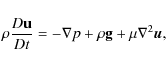 |
(1) |
where
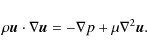
A useful parameter in hydrodynamics theory is the Reynolds number

where d is a characteristic length of the body, U the speed, and
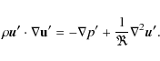
On the other hand, for low Reynolds number (
From Eqs. (4) and (5), it is possible to derive the expressions for the force acting on a body in a ``laminar'' (low
and
In Eqs. (6) and (7), the indexs l and t refers to laminar and turbulent regime,
2.3 Variability of ICME radius
We used the expressions for the drag forces
(Eqs. (6) and (7))
in the equation of motion. We also consider that the ICME radius (R) varies with the distance as R=xp, assuming p=0.78(Liu et al. 2005).
In a system of reference where the ambient SW is at
rest, and therefore,
the ICME speed is
![]() ,
where
,
where
![]() is the solar wind speed,
we obtain the following differential equations for ``laminar'' and
``turbulent'' regimes:
is the solar wind speed,
we obtain the following differential equations for ``laminar'' and
``turbulent'' regimes:
and
Solutions of Eqs. (8) and (9) are given by
![$\displaystyle x^{(p+1)}- x_{0}^{(p+1)}= - \frac{m_{\rm cme} (p+1)}{6 \pi \mu} \...
...+U_{\rm sw} \ln\left[\frac{(U-U_{\rm sw})}{(U_{0} - U_{\rm sw})}\right]}\right)$](/articles/aa/full_html/2009/18/aa11171-08/img46.png)
and
![$\displaystyle x^{(2p+1)}-x_{0}^{(2p+1)}= -2 \frac{m_{\rm cme} (2p+1)}{C_{\rm d}...
...sw})} + \ln \left[ \frac{(U-U_{\rm sw})}{(U_{0}-U_{\rm sw})}\right]\right]\cdot$](/articles/aa/full_html/2009/18/aa11171-08/img47.png)
In Eqs. (10) and (11), U0 and x0 are the initial CME speed and position
(as measured at the coronograph field of view).
To analyze the motion described by Eqs. (10) and (11),
we present in Figs. 1 and 2 the resulting speed as a function of the position, for different initial speeds, considering
![]() .
The plots are for two different values of
.
The plots are for two different values of
![]() (continuous lines) and
(continuous lines) and
![]() (dotted lines); and
(dotted lines); and
![]() (continuous lines) and
(continuous lines) and
![]() (dotted lines). In all cases, we have chosen the parametres (
(dotted lines). In all cases, we have chosen the parametres (![]() and
and ![]() )
in such a way that the ICME speed at 1 AU fall in a range similar to the observed (see Paper 1 for more details).
)
in such a way that the ICME speed at 1 AU fall in a range similar to the observed (see Paper 1 for more details).
![\begin{figure}
\par\includegraphics[width=7cm,clip]{f1_1171.eps}
\end{figure}](/articles/aa/full_html/2009/18/aa11171-08/img51.png) |
Figure 1:
ICME speed versus distance
for ``laminar regime'', showing a weak (
|
| Open with DEXTER | |
![\begin{figure}
\par\includegraphics[width=7cm,clip]{f2_1171.eps}
\end{figure}](/articles/aa/full_html/2009/18/aa11171-08/img52.png) |
Figure 2:
ICME speed versus distance for ``turbulent regime'',
showing a weak (
|
| Open with DEXTER | |
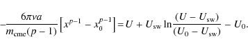
2.4 Density variation in the interplanetary medium
To improve the analysis, we used the
Leblanc et al. (1996) model to account for the variation in the SW
density with the distance, given by

where
2.4.1 ``Turbulent'' regime
The ``turbulent'' regime, described by Eq. (7),
has an explicit dependence with the density, therefore, by using
![]() we obtain the following equation
we obtain the following equation
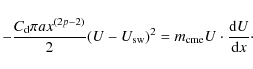
The solution is given by
![$\displaystyle -\frac{C_{\rm d} \pi a} {2 m_{\rm cme} (2p-1)} \left[x^{(2p-1)}-x...
...-U_{\rm sw})}+ \ln \left[ \frac{(U-U_{\rm sw})}{(U_{0}-U_{\rm sw})}\right]\cdot$](/articles/aa/full_html/2009/18/aa11171-08/img61.png)
The behavior of the speed versus position, given by Eq. (14), can be seen in Fig. 3, where we have plotted the solutions for different initial speeds and using two drag coefficients,
![\begin{figure}
\par\includegraphics[width=7cm]{f3_1171.eps}
\end{figure}](/articles/aa/full_html/2009/18/aa11171-08/img64.png) |
Figure 3:
ICME speed versus distance for ``turbulent regime''
considering ICME radius and SW density variable. The ICME - SW interaction is
weak for a drag coefficient
|
| Open with DEXTER | |
2.4.2 ``Laminar'' regime
To describe the motion of the ICMEs considering the ``laminar'' regime, it is
necessary to express the ``laminar'' force as a function of the density of the
medium (in this case the SW density). Therefore, we use
the relationship between the dynamic viscous coefficient ![]() and the
kinematic viscous coefficient
and the
kinematic viscous coefficient ![]() ,
as (see Kundu & Cohen 2004, for details):
,
as (see Kundu & Cohen 2004, for details):

Using Eq. (15), the equation of motion becomes
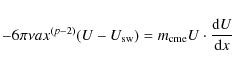 |
(16) |
and the solution is
Finally, the behavior of the speed versus position for this case can be seen in Fig. 4, where we have plotted the solution (Eq. (17)) for different initial speeds and using a value of
![\begin{figure}
\par\includegraphics[width=7cm]{f4_1171.eps}
\end{figure}](/articles/aa/full_html/2009/18/aa11171-08/img71.png) |
Figure 4:
ICME speed versus distance for ``laminar regime'' considering
ICME radius and SW density variable, in this case the value of the
kinematic viscosity is
|
| Open with DEXTER | |
3 Discussion and conclusion
The acceleration in the interplanetary medium of CMEs is well-established
(Manoharan 2006; Howard 2007; Gopalswamy et al. 2000,2001; Manoharan et al. 2001).
This acceleration has been explained by an increase of the ICME mass (snow-plough model Tappin 2006) or due to Lorentz force (Chen 1996; Howard 2007), although it is more common to attribute this acceleration to drag forces (Vrsnak 2001; Cargill 2004).
However, the exact form, the magnitude of the related coefficients and
the dependence of this drag force with the CME or SW parameters are still unknown. Even more, there are doubts about this force acting on ICMEs
(Forbes et al. 2006; Reiner et al. 2003).
As pointed out by Vrsnak et al. (2006), by considering the kinetic energy of
ICMEs, the gravity and Lorentz forces are negligible in the interplanetary space.
Therefore, a drag force should act in the interchange of momentum between the ICME and the SW.
All forces, Lorentz, aerodynamic drag, and gravity, decrease with the
heliocentric distance (Chen 1996; Sheeley et al. 1997; Chen 1993; Vrsnak et al. 2006). Although, the Lorentz force is
the most important at low heights then the drag becomes
predominant after
![]() (Vrsnak et al. 2006).
Recently, to explain IPS and white light observations (SMEI), Howard (2007)
has suggested that the drag force overcome the Lorentz force at
greater distances, between 80 to
(Vrsnak et al. 2006).
Recently, to explain IPS and white light observations (SMEI), Howard (2007)
has suggested that the drag force overcome the Lorentz force at
greater distances, between 80 to
![]() .
Here, since we are not taking the magnetic field effects into account, we neglect the Lorentz force.
In order to understand and model the drag force acting on the ICME-SW system,
we explore two
forms of this force (linearly and quadratically dependent with the ICME speed)
and variations in two parameters of the system (the CME radius and
the SW density). Our analytical analysis helps to physically
understand the effects of these parameters and dependences in the ICME
dynamics.
To perform such comparison, in Fig. 5 we plot
Eqs. (10), (11), (14), and (17), assuming an initial speed of 1000 km s-1and the parameters (
.
Here, since we are not taking the magnetic field effects into account, we neglect the Lorentz force.
In order to understand and model the drag force acting on the ICME-SW system,
we explore two
forms of this force (linearly and quadratically dependent with the ICME speed)
and variations in two parameters of the system (the CME radius and
the SW density). Our analytical analysis helps to physically
understand the effects of these parameters and dependences in the ICME
dynamics.
To perform such comparison, in Fig. 5 we plot
Eqs. (10), (11), (14), and (17), assuming an initial speed of 1000 km s-1and the parameters (![]() and
and ![]() )
corresponding to the mean values of these
parameters used in Figs. 1 to 4.
Upon inspection of Fig. 5, it is easy to see a completely
different behavior between the models considering only variability of
the ICME radius and considering variability of both,
ICME radius and solar wind density.
)
corresponding to the mean values of these
parameters used in Figs. 1 to 4.
Upon inspection of Fig. 5, it is easy to see a completely
different behavior between the models considering only variability of
the ICME radius and considering variability of both,
ICME radius and solar wind density.
![\begin{figure}
\par\includegraphics[width=7cm]{f5_1171.eps}
\end{figure}](/articles/aa/full_html/2009/18/aa11171-08/img76.png) |
Figure 5:
ICME speed versus distance for the
four models analyzed in this work.
a) ``laminar'' regime considering variability in ICME radius (Eq. (10))
and
|
| Open with DEXTER | |
When the dominant variation is the CME radius (as x0.78), the curves have negative concavity; when the density variation (as x-2) is dominant, the concavity changes, meaning that the density of the medium plays an important role in the transport of the ICMEs (Reiner et al. 2003).
Using scintillation data (IPS), Manoharan et al. (2001) and
Manoharan (2006) have found that ICMEs show a low decline in speed below
100 ![]() (
(
![]() )
and a rapid decrease after this distance.
This behavior agree with the concavity of the curves in
Figs. 1 and 2. By analyzing type II bursts, Reiner et al. (2003) find that a drag force cannot
explain the observed frequency drift. They argue that
a change in the concavity of the velocity-distance curve is necessary in order to fit the
type II data. We note that Reiner et al. (2003) used similar
variations for both CME area (
)
and a rapid decrease after this distance.
This behavior agree with the concavity of the curves in
Figs. 1 and 2. By analyzing type II bursts, Reiner et al. (2003) find that a drag force cannot
explain the observed frequency drift. They argue that
a change in the concavity of the velocity-distance curve is necessary in order to fit the
type II data. We note that Reiner et al. (2003) used similar
variations for both CME area (
![]() )
and SW density (
)
and SW density (
![]() ).
Here we show that it is necessary to determine the dominant parameter
in the drag force in order to determine the concavity of the curve.
Considering the ``turbulent'' regime and
using the variation in radius as the dominant factor, we note the drag-coefficient
between
).
Here we show that it is necessary to determine the dominant parameter
in the drag force in order to determine the concavity of the curve.
Considering the ``turbulent'' regime and
using the variation in radius as the dominant factor, we note the drag-coefficient
between
![]() ;
on the other hand,
if we consider the density variation as the dominant factor,
the drag's coefficient values diminish to the
;
on the other hand,
if we consider the density variation as the dominant factor,
the drag's coefficient values diminish to the
![]() -
-
![]() range.
range.
Acknowledgements
A. Borgazzi acknowledges grant CNPq-Brazil. A. Lara acknowledges UNAM-PAPIIT grant IN117309 and CONACyT grants 49395 and 42577 for partial support. E. Echer would like to thank the Brazilian CNPq (PQ-300104/2005-7 and 470706/2006-6) agencies for financial support. M.V. Alves thanks the support given by CNPq (304865/2007-9).
References
- Batchelor, G. K. 2000, An Introduction to fluid dynamics (Cambridge University Press)
- Borgazzi, A., Lara, A., Romero-Salazar, L., & Ventura, A. 2008, Geof. Int., 47, 301 [NASA ADS] (In the text)
- Canto, J., Gonzalez, R. F., Raga, A. C., et al. 2005, MNRAS, 357, 572 [NASA ADS] [CrossRef] (In the text)
- Chen, J. 1996, J. Geophys. Res., 101, A12, 27499 (In the text)
- Chen, J., & Garren, D. 1993, Geophys. Res. Lett., 20, 21 [CrossRef], 2319 (In the text)
- Cargill, P. J. 2004, Sol. Phys., 221, 135 [NASA ADS] [CrossRef]
- Cargill, P. J., & Chen, J. 1996, J. Geophys. Res., 101, A3 [CrossRef], 4855
- Daugherty, R., Franzini, J., & Finnemore, E. 1989, Fluid Mechanics with Engineering Applications (McGraw-Hill Book Company) (In the text)
- Forbes, T. G., Linker, J. A., Chen, J., et al. 2006, Space Sc. Rev., 123, 1 [NASA ADS] [CrossRef], 251
- Gonzalez-Esparza, A., Lara, A., Perez-Tijerina, E., Santillan, A., & Gopalswamy, N. 2003, J. Geophys. Res., 108, A1 [CrossRef]
- Gopalswamy, N., Lara, A., Lepping, R. P., et al. 2000, Geophys. Res. Lett., 27, 145 [NASA ADS] [CrossRef]
- Gopalswamy, N., Lara, A., Yashiro, S., Kaiser, M. L., & Russell, H. 2001, J. Geophys. Res., 18, 29.207
- Gopalswamy, N., Lara, A., Manoharan, P., & Howard, R. 2005, Adv. Space Res., 36, 2289 [CrossRef]
- Gosling, J. T., McComas D. J., Phillips, J. L., & Bame, S. J. 1999, J. Geophys. Res., 96, A5, 7831 (In the text)
- Howard, T., Fry, C., & Webb, D. 2007, ApJ., 667, 610 [NASA ADS] [CrossRef]
- Kundu, P., & Cohen, I. 2004, Fluid Mechanics (Elsevier Academic Press), third edition (In the text)
- Landau, L., & Lifshitz, M. 1987, Fluid Mechanics (Pergamon Press), second edition (In the text)
- Leblanc, Y., Dulk, G., & Bougeret, J. 1996, Sol. Phys., 183, 165 [NASA ADS] [CrossRef] (In the text)
- Liu, I., Richardson, J. D., & Belcher, J. W. 2005, Planetary and Space Science, 53, 3 [NASA ADS] [CrossRef] (In the text)
- Manoharan, P. 2006, Sol. Phys., 235, 345 [NASA ADS] [CrossRef] (In the text)
- Manoharan, P., Tokumaru, M., Pick, M., et al. 2001, ApJ, 559, 1180 [NASA ADS] [CrossRef]
- Odstr
 il, D., & Pizzo, V. J. 1999a, J. Geophys. Res., 104,
A1 [CrossRef], 483
il, D., & Pizzo, V. J. 1999a, J. Geophys. Res., 104,
A1 [CrossRef], 483
- Odstr
il, D., & Pizzo, V. J. 1999b, J. Geophys. Res., 104,
A1 [CrossRef], 493
- Reiner, M. J., Kaiser, M. L., & Bougeret, J. L. 2003, in Solar Wind Ten, ed. M. Velli, et al., AIP Conf. Proc., 679, 152
- St. Cyr, O. C., Burkepile, J. T., Hundhausen, A. J., & Lecinski, A. R. 1999, J. Geophys. Res., 104 ,A6 , 12493
- Sheeley, N. R., Wang, Jr., Hawley, S. H., et al. 1997, ApJ, 484, 472 [NASA ADS] [CrossRef] (In the text)
- Tappin, S. 2006, Sol. Phys., 233, 233 [NASA ADS] [CrossRef] (In the text)
- Tappin, S., Buffington, A., Cooke, C., et al. 2006, Geophys. Res. Lett., 31, L02802 [CrossRef] (In the text)
- Vandas, M., Fisher, S., Dryer, M., Smith, M., & Detman, T. 1995, J. Geophys. Res., 100, A7, 12258
- Vr
 nak, B. 2001, J. Geophys. Res., 106, A11, 25249
- Vr
nak, B. 2006, Adv. Space Res., 38, 431 [NASA ADS] [CrossRef]
(In the text)
- Vr
nak, B., & Gopalswamy, N. 2002, J. Geophys. Res.,
107, A2
- Vr
nak, B., &
 ic, T. 2007, A&A, 472, 937 [NASA ADS] [CrossRef] [EDP Sciences]
- Vr
nak, B., Ru
 djak, D., Sudar, D., & Gopalswamy, N. 2004, A&A,
423, 717 [NASA ADS] [CrossRef] [EDP Sciences]
djak, D., Sudar, D., & Gopalswamy, N. 2004, A&A,
423, 717 [NASA ADS] [CrossRef] [EDP Sciences]
All Figures
| |
Figure 1:
ICME speed versus distance
for ``laminar regime'', showing a weak (
|
| Open with DEXTER | |
| In the text | |
| |
Figure 2:
ICME speed versus distance for ``turbulent regime'',
showing a weak (
|
| Open with DEXTER | |
| In the text | |
| |
Figure 3:
ICME speed versus distance for ``turbulent regime''
considering ICME radius and SW density variable. The ICME - SW interaction is
weak for a drag coefficient
|
| Open with DEXTER | |
| In the text | |
| |
Figure 4:
ICME speed versus distance for ``laminar regime'' considering
ICME radius and SW density variable, in this case the value of the
kinematic viscosity is
|
| Open with DEXTER | |
| In the text | |
| |
Figure 5:
ICME speed versus distance for the
four models analyzed in this work.
a) ``laminar'' regime considering variability in ICME radius (Eq. (10))
and
|
| Open with DEXTER | |
| In the text | |
Copyright ESO 2009
Current usage metrics show cumulative count of Article Views (full-text article views including HTML views, PDF and ePub downloads, according to the available data) and Abstracts Views on Vision4Press platform.
Data correspond to usage on the plateform after 2015. The current usage metrics is available 48-96 hours after online publication and is updated daily on week days.
Initial download of the metrics may take a while.