| Issue |
A&A
Volume 498, Number 2, May I 2009
|
|
|---|---|---|
| Page(s) | 661 - 665 | |
| Section | Numerical methods and codes | |
| DOI | https://doi.org/10.1051/0004-6361/200810885 | |
| Published online | 19 March 2009 | |
A Field-length based refinement criterion for adaptive mesh simulations of the interstellar medium
(Research Note)
O. Gressel1,2
1 - Astrophysikalisches Institut Potsdam, An der Sternwarte 16, 14482 Potsdam, Germany
2 - Astronomy Unit, School of Mathematical Sciences, Queen Mary, University of London, Mile End Road, London E1 4NS, UK
Received 1 September 2008 / Accepted 2 February 2009
Abstract
Context. Adequate modelling of the multiphase interstellar medium requires optically thin radiative cooling, containing an inherent thermal instability. The size of the resulting condensation and evaporation interfaces is determined by the so-called Field-length, which represents the dimension across which the instability is damped significantly by thermal conduction.
Aims. We study the relevance of conduction scale effects in the numerical modelling of a bistable medium and check the applicability of conventional and alternative adaptive mesh techniques.
Methods. The low value of the thermal conduction coefficient in the ISM defines a multiscale problem, promoting the use of adaptive meshes. We introduce a refinement strategy that applies the Field condition by Koyama & Inutsuka as a refinement criterion. The described method is similar to the Jeans criterion for gravitational instability by Truelove and allows us to trace efficiently the unstable gas situated at the thermal interfaces.
Results. We present test computations that demonstrate the higher accuracy of our proposed refinement criterion compared to refinement based on the local density gradient. Apart from its usefulness as a refinement trigger, we do not find evidence in favour of the Field criterion being a prerequisite for numerical stability.
Key words: hydrodynamics - instabilities - ISM: general - ISM: structure
1 Introduction
The structure of the turbulent interstellar medium (ISM) of the Milky Way and other disk galaxies is determined by various complex physical processes. In particular, the formation of the neutral atomic phase of the ISM is believed to be regulated by condensation under the action of thermally bistable radiative cooling. The related thermal instability (TI) has been studied extensively as a modifying agent for various driving sources of turbulence in the ISM. Numerical studies have included the magneto-rotational instability (MRI) (Piontek & Ostriker 2007,2005), explosions of SNe (Gressel et al. 2008b; Korpi et al. 1999; de Avillez & Breitschwerdt 2005; Joung & Mac Low 2006; Gressel et al. 2008a), and converging flows (; Audit & Hennebelle 2005; Vázquez-Semadeni et al. 2006). Adaptive mesh MHD simulations of the last scenario were performed by Hennebelle et al. (2008), who applied a simple density threshold as a refinement criterion.
The development of TI alone was explored under various conditions by Sánchez-Salcedo et al. (2002). Moreover, there was a discussion of whether TI in conjunction with thermal conduction can act as an independent source of turbulence (Brandenburg et al. 2007; Koyama & Inutsuka 2006).
In dynamic simulations of the ISM, the radiative cooling is usually
treated in the limit of an optically thin plasma, i.e., radiative
transport effects are neglected. The cooling rate is then prescribed
by
![]() in units of
in units of
![]() .
Here we adopt
the cooling function from Sánchez-Salcedo et al. (2002) that is a
piecewise power-law fit to results by Wolfire et al. (1995).
.
Here we adopt
the cooling function from Sánchez-Salcedo et al. (2002) that is a
piecewise power-law fit to results by Wolfire et al. (1995).
In this paper, we focus on an issue in the numerical treatment of
thermally bistable gas first brought up by Koyama & Inutsuka (2004). The comprehensive theoretical analysis by Field (1965) reveals that, in the case of vanishing
thermal conduction, TI has a finite growth rate in the limit of high
wave numbers. In the discrete representation of the fluid, this
implies that numerical fluctuations on grid scale will be prone to
artificial amplification by the physical instability unless
appropriate precautions are taken. The most natural way to guarantee a
physically meaningful, converged solution is to introduce a physically
motivated dissipation length that must then be resolved on the numerical grid. When thermal conduction cannot be neglected, Field (1965) derived a stability criterion for the condensation mode of the general form
![]() where
where ![]() is the coefficient of thermal conduction in units of
is the coefficient of thermal conduction in units of
![]() .
For a power-law cooling function
.
For a power-law cooling function
![]() ,
this reduces to
,
this reduces to
![]() .
The wavelength
.
The wavelength
![]() at which the criterion is fulfilled marginally defines the scale on which fluctuations generated by the TI are efficiently damped by thermal conduction. Koyama & Inutsuka (2004) demonstrated that
at which the criterion is fulfilled marginally defines the scale on which fluctuations generated by the TI are efficiently damped by thermal conduction. Koyama & Inutsuka (2004) demonstrated that
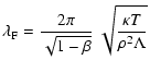
must be resolved with at least three grid cells to attain a converged numerical solution. It occurs naturally to use this criterion as a condition for mesh refinement.
2 Numerical methods
For our simulations, we use the NIRVANA code, which is a general-purpose MHD fluid tool designed to solve multiscale, self-gravitating hydrodynamics problems. The NIRVANA code comprises (i) a fully conservative, divergence-free Godunov-type central scheme (Ziegler 2004); (ii) a block-structured adaptive mesh refinement (AMR), and (iii) a multigrid-like adaptive mesh Poisson solver with elliptic matching (Ziegler 2005).
The central aim of adaptive mesh simulations is to resolve regions of interest at enhanced accuracy. In AMR codes such as Enzo (O'Shea et al. 2004), FLASH (Fryxell et al. 2000), NIRVANA, or RAMSES (Teyssier 2002), this can be achieved by applying a variety of different criteria: baryon or dark matter overdensity (cosmological structure formation), local Jeans-length (protostellar core collapse), or entropy gradients (accretion shocks). Iapichino et al. (2008) introduced a vorticity-based criterion to properly resolve a turbulent wake. Alternatively, and independently of the underlying physics, the amount of discrepancy between the solutions on different AMR levels can be used as an indication for refinement (Berger & Colella 1989).
2.1 Classical mesh refinement
As a standard criterion for tracing developing structures, one typically monitors local gradients ![]() in the fluid variables u. To be able to follow moving structures (and anticipate emerging structures), it is furthermore desirable to consider the temporal change in these gradients. Because of the additional overhead in storing quantities between timesteps, this is usually omitted, and one assumes that strong gradients are bordered by sections of enhanced curvature, as reflected in the second derivatives
in the fluid variables u. To be able to follow moving structures (and anticipate emerging structures), it is furthermore desirable to consider the temporal change in these gradients. Because of the additional overhead in storing quantities between timesteps, this is usually omitted, and one assumes that strong gradients are bordered by sections of enhanced curvature, as reflected in the second derivatives ![]() .
Accordingly, NIRVANA's usual mesh refinement is determined by combining the criterion of normalised gradients
.
Accordingly, NIRVANA's usual mesh refinement is determined by combining the criterion of normalised gradients
![]() with one of the ratio of second to first derivatives
with one of the ratio of second to first derivatives
![]() of the conserved variables u, i.e.,
of the conserved variables u, i.e.,
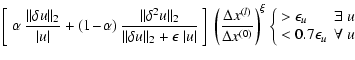
where
For our runs not based on the Field condition, we adopt refinement for the gas density ![]() only and use trigger values
only and use trigger values
![]() of 0.02 and 0.04 while we set
of 0.02 and 0.04 while we set
![]() .
Including the ratio of grid spacings
.
Including the ratio of grid spacings ![]() of refinement level l to the base level enables a level-dependent refinement via the choice of the exponent
of refinement level l to the base level enables a level-dependent refinement via the choice of the exponent ![]() .
Here we fix
.
Here we fix ![]() ,
which makes refinements on higher levels successively easier. Finally, we set the additional filter value
,
which makes refinements on higher levels successively easier. Finally, we set the additional filter value
![]() to prevent the refinement of small ripples.
to prevent the refinement of small ripples.
| |
Figure 1:
Effect of the adjustable parameters |
| Open with DEXTER | |
While this general form of the refinement criterion is very flexible, the large number of free parameters renders the optimal adjustment to a particular problem a tedious task requiring a certain amount of experience. Since AMR always implies a trade-off between accuracy and efficiency, the optimal choice is also by no means clear-cut. This is illustrated in Fig. 1, where we show the variation in the accuracy and AMR speed-up![]() as a function of the two supplementary parameters
as a function of the two supplementary parameters ![]() and
and ![]() of the classical refinement estimator (2). In principle, one can use these graphs to find the parameter set that yields the highest execution speed at a given level of fidelity. However, this procedure remains limited to simple test cases, and its universality cannot be easily proven.
of the classical refinement estimator (2). In principle, one can use these graphs to find the parameter set that yields the highest execution speed at a given level of fidelity. However, this procedure remains limited to simple test cases, and its universality cannot be easily proven.
2.2 Refinement based on the Field condition
In an alternative approach tailored to tracing condensation interfaces, we apply grid refinement wherever the local Field-length
![]() is not resolved by at least three grid cells. For fine tuning,
this number can be varied as a linear function of the refinement level, although we do not use this dispensable feature here. The main advantage of the proposed new method is that it is virtually parameter free. This implies that the intricate determination of suitable values
for
is not resolved by at least three grid cells. For fine tuning,
this number can be varied as a linear function of the refinement level, although we do not use this dispensable feature here. The main advantage of the proposed new method is that it is virtually parameter free. This implies that the intricate determination of suitable values
for ![]() and
and ![]() (as described above) can be avoided.
(as described above) can be avoided.
The evaluation of
![]() ,
given by Eq. (1), is straightforward since the values of
,
given by Eq. (1), is straightforward since the values of ![]() and T have already been computed for the heat flux term. To minimise overheads, they are
stored in auxiliary arrays. It is evident that the definition of the Field-length requires the inclusion of a heat conduction term in the energy equation. In contrast to this, the FLASH code supports refinement based on the local cooling time
and T have already been computed for the heat flux term. To minimise overheads, they are
stored in auxiliary arrays. It is evident that the definition of the Field-length requires the inclusion of a heat conduction term in the energy equation. In contrast to this, the FLASH code supports refinement based on the local cooling time
![]() ,
which is independent of
,
which is independent of ![]() .
In our case, if
.
In our case, if ![]() is scaled by
is scaled by ![]() (see below), the two methods should perform similarly.
(see below), the two methods should perform similarly.
3 Results
3.1 Gaussian density perturbation
![\begin{figure}
\par\includegraphics[width=8.8cm,clip]{fig/0885fig2}
\end{figure}](/articles/aa/full_html/2009/17/aa10885-08/img39.gif) |
Figure 2:
Field-length as a function of radius for the problem DEN3
described in Sánchez-Salcedo et al. (2002) for the initial profile (dashed lines), and the final profile at
|
| Open with DEXTER | |
As a test problem, we revisit the 1D case of a density perturbation as
considered in the model DEN3 from Sánchez-Salcedo et al. (2002, hereafter SSVSG). In this setup, a gas of density
![]() initially rests at its equilibrium pressure of
initially rests at its equilibrium pressure of
![]() and is perturbed by a Gaussian overdensity of amplitude
0.2, FWHM of
and is perturbed by a Gaussian overdensity of amplitude
0.2, FWHM of ![]() ,
and centred within a domain of
,
and centred within a domain of
![]() .
Unlike
in our simulations, SSVSG do not apply thermal conduction. This means
that we must apply a high enough resolution so that conduction (which
becomes important mainly on the grid scale) does not affect
significantly the features seen in their solution. As a reference, we
perform a uni-grid run at a linear resolution of 8192 cells,
corresponding to a grid spacing of
.
Unlike
in our simulations, SSVSG do not apply thermal conduction. This means
that we must apply a high enough resolution so that conduction (which
becomes important mainly on the grid scale) does not affect
significantly the features seen in their solution. As a reference, we
perform a uni-grid run at a linear resolution of 8192 cells,
corresponding to a grid spacing of ![]()
![]() .
The
level of conduction is then chosen in such a way that
.
The
level of conduction is then chosen in such a way that
![]() is resolved properly in the reference run. This yields a value for
is resolved properly in the reference run. This yields a value for ![]() which is about a factor of 500 higher than the physical
Spitzer value in the limit of vanishing electron density. Thus, the
even smaller structures expected in a physically meaningful scenario
illustrate the need for applying multiscale techniques.
which is about a factor of 500 higher than the physical
Spitzer value in the limit of vanishing electron density. Thus, the
even smaller structures expected in a physically meaningful scenario
illustrate the need for applying multiscale techniques.
Figure 2 shows a plot of the Field-length for the
initial and final density and temperature profiles, where we use three
different prescriptions for the conduction. Scaling ![]() by
by ![]() is typically used in combination with a constant kinematic viscosity
yielding a constant value for the Prandtl number and a constant numerical time step, which is computationally favourable. This is also reflected in the Field-length varying only weakly with density. For the case of constant
is typically used in combination with a constant kinematic viscosity
yielding a constant value for the Prandtl number and a constant numerical time step, which is computationally favourable. This is also reflected in the Field-length varying only weakly with density. For the case of constant ![]() ,
this variation is stronger and accounts
for about one order of magnitude in the problem under consideration. Finally, for a Spitzer-type conductivity of
,
this variation is stronger and accounts
for about one order of magnitude in the problem under consideration. Finally, for a Spitzer-type conductivity of
![]() ,
we obtain a variation of over two orders of magnitude in
,
we obtain a variation of over two orders of magnitude in
![]() rendering this case particularly interesting for AMR. In the following, we restrict ourselves to the case of a constant coefficient
rendering this case particularly interesting for AMR. In the following, we restrict ourselves to the case of a constant coefficient
![]() .
.
![\begin{figure}
\par\includegraphics[width=17cm,clip]{fig/0885fig3}
\end{figure}](/articles/aa/full_html/2009/17/aa10885-08/img48.gif) |
Figure 3:
Temporal evolution of density ( left), thermal pressure
( centre), and velocity ( right), for our 512+4 run with constant |
| Open with DEXTER | |
In general, the results are only marginally affected when conduction
is included and agree well with the solution of SSVSG. In
Fig. 3, the resulting profiles for the run with
a 512 cell base-grid plus 4 levels of refinement (based on the Field
condition) are plotted. Before we proceed with an analysis of the AMR
performance, we want to compare our reference run 8192+0 (which is
barely distinguishable from the one shown in Fig. 3) with the profiles from SSVSG: the most noticeable discrepancy is in the overall level of the thermal pressure. Due to the assumed periodicity at the domain boundaries, the mean pressure becomes a highly fluctuating quantity (cf. central panel of Fig. 3). Apart from the different offsets, the pressure profiles match reasonably well. We note that there is a small pressure dip at the interface of the condensed structure in our results that is not seen in SSVSG. A similar feature is observed in panel (d) of their Fig. 7 (model DEN75), although much spikier. This leaves the possibility that the feature is not resolved by the plot for model DEN3 in Fig. 2 of SSVSG. A comparison run with ![]() in fact shows that, in our setup, the dip is broadened by the thermal conduction and otherwise remains much narrower. Later investigations of the topic consistently reveal a similar region of lower pressure (see e.g., Vázquez-Semadeni et al. 2003), which can be attributed to
the pressure decreasing with density in the unstable regime. In this respect, the pressure dip reflects the S-shape of the equilibrium cooling curve.
in fact shows that, in our setup, the dip is broadened by the thermal conduction and otherwise remains much narrower. Later investigations of the topic consistently reveal a similar region of lower pressure (see e.g., Vázquez-Semadeni et al. 2003), which can be attributed to
the pressure decreasing with density in the unstable regime. In this respect, the pressure dip reflects the S-shape of the equilibrium cooling curve.
In Fig. 4, we plot the relative errors of three AMR
runs with respect to the fully resolved solution. The two panels
correspond to the two intervals with the strongest deviations, i.e.,
an outgoing wave (upper panel) and the condensation interface of the
cloud (lower panel). We compare the two runs based on the density
gradient criterion (with
![]() and 0.04) with the
run based on the Field condition. At the time
and 0.04) with the
run based on the Field condition. At the time
![]() ,
the number
of AMR blocks for these runs are 820, 476, and 504, respectively. Although the number of refined cells is comparable, the Field condition yields a relative error that is lower by a factor of
two at the condensation front. For
,
the number
of AMR blocks for these runs are 820, 476, and 504, respectively. Although the number of refined cells is comparable, the Field condition yields a relative error that is lower by a factor of
two at the condensation front. For
![]() (0.02),
the outgoing wave is resolved at l=1 (3), while the Field
condition, as expected, is insensitive to this feature and does not
trigger refinement at all. Yet the relative error is the lowest in
this case, indicating that the wave might be overly steepened by the
refinement based on the density gradients. This finding is rather
surprising and requires further investigation.
(0.02),
the outgoing wave is resolved at l=1 (3), while the Field
condition, as expected, is insensitive to this feature and does not
trigger refinement at all. Yet the relative error is the lowest in
this case, indicating that the wave might be overly steepened by the
refinement based on the density gradients. This finding is rather
surprising and requires further investigation.
4 Discussion
As illustrated in Fig. 5, thermal fragmentation produces turbulent and extremely filamentary structures. Since turbulence can be modelled properly only in three dimensions, adaptive mesh refinement becomes highly beneficial, if not mandatory. Because classical refinement strategies reach their limits if turbulence is involved (see e.g., Iapichino et al. 2008, for a vorticity-based refinement criterion), one must seek new tracers of structural properties. This is particularly true in the case of a thermally unstable medium.
Until now, the criterion introduced by Koyama & Inutsuka (2004) has been widely disregarded by many members of the numerical astrophysics community. Notable exceptions are a TI study by Brandenburg et al. (2007) and the MRI simulations of Piontek & Ostriker (2004). The opposite standpoint, represented by a number of authors (see e.g., Gazol et al. 2005; Joung & Mac Low 2006), is to neglect thermal conduction altogether. The standard argument is that numerical diffusion defines a ``numerical Field-length'' that is believed to damp down small-scale modes of the instability sufficiently. On the other hand, de Avillez & Breitschwerdt (2004) argued that microscopic heat conduction is suppressed perpendicular to the magnetic field lines (and thus also isotropically for sufficiently tangled fields) and that turbulent transport plays an important role. Although this is certainly true, it does not aid the discussion of whether explicit conduction should be included.
In our own simulations, we observe artificial growth of modes close to the resolution limit only in situations where the Courant number is chosen to be inappropriately high or the gradient-based refinement criterion is adjusted improperly. The absence of unphysical growth at high wavenumbers might thus, in fact, be attributed to the finite level of numerical dissipation, which is never really negligible in 3D simulations.
![\begin{figure}
\par\includegraphics[width=8cm]{fig/0885fig4}
\end{figure}](/articles/aa/full_html/2009/17/aa10885-08/img51.gif) |
Figure 4:
Relative errors of the density profiles at time
|
| Open with DEXTER | |
![\begin{figure}
\par\includegraphics[width=8cm,clip]{fig/0885fig5}
\end{figure}](/articles/aa/full_html/2009/17/aa10885-08/img53.gif) |
Figure 5:
The Field-length criterion in action: development of the
thermal instability from random fluctuations with Spitzer-type conductivity. The 2D simulation has a base grid of 2562 with refinement of up to 8 levels, covering scales from 0.003-
|
| Open with DEXTER | |
In this respect, the Field criterion of Koyama & Inutsuka appears to be of academic interest only. Apart from its true necessity, we have however demonstrated that the condition can be used successfully as a refinement criterion for adaptive mesh simulations of the interstellar medium, an approach that is similar to the refinement procedure based on the Jeans-length introduced by Truelove et al. (1997) for self-gravitating clouds. In a simple 1D test case, the new refinement estimator is found to produce more accurate results at comparable numerical cost than conventional criteria.
The overhead of evaluating
![]() is low compared to the computation of
the numerical fluxes. Within NIRVANA, the determination of the heat
flux already requires the evaluation of the gas temperature and the
(non-uniform) conductivity coefficient. These fields can therefore be
stored temporarily such that the only additional expense comes from
evaluating the cooling function.
is low compared to the computation of
the numerical fluxes. Within NIRVANA, the determination of the heat
flux already requires the evaluation of the gas temperature and the
(non-uniform) conductivity coefficient. These fields can therefore be
stored temporarily such that the only additional expense comes from
evaluating the cooling function.
The definition of
![]() nevertheless implies the inclusion of thermal
conduction, which is not a standard feature in many available
codes. An alternative approach (implemented in the FLASH code) is
instead to use the cooling time, which is independent of
nevertheless implies the inclusion of thermal
conduction, which is not a standard feature in many available
codes. An alternative approach (implemented in the FLASH code) is
instead to use the cooling time, which is independent of ![]() .
On
the other hand, there is evidence (Piontek, in prep.) that heat
conduction is in fact physically relevant to the formation of
molecular clouds, providing further motivation for the use of the
proposed scheme.
.
On
the other hand, there is evidence (Piontek, in prep.) that heat
conduction is in fact physically relevant to the formation of
molecular clouds, providing further motivation for the use of the
proposed scheme.
Compared to classical mesh refinement based on gradients, which has to be fine-tuned by multiple parameters according to different situations, the Field criterion is virtually parameter-free and provides reliable results irrespective of the particular setup. If it becomes mandatory to adequately resolve features such as shock fronts, one must, of course, still rely on a combination with conventional refinement criteria. This does, however, not impose any difficulties.
Acknowledgements
This work made use of the NIRVANA code developed by Udo Ziegler at the Astrophysical Institute Potsdam. I thank Enrique Vázquez-Semadeni and Simon Glover for discussions related to this work and acknowledge the helpful comments by the anonymous referee.
References
- Audit, E., & Hennebelle, P. 2005, A&A, 433, 1 [NASA ADS] [CrossRef] [EDP Sciences]
- Berger, M. J., & Colella, P. 1989, JCoPh, 82, 64 [NASA ADS] (In the text)
- Brandenburg, A., Korpi, M. J., & Mee, A. J. 2007, ApJ, 654, 945 [NASA ADS] [CrossRef]
- de Avillez, M. A., & Breitschwerdt, D. 2004, A&A, 425, 899 [NASA ADS] [CrossRef] [EDP Sciences]
- de Avillez, M. A., & Breitschwerdt, D. 2005, A&A, 436, 585 [NASA ADS] [CrossRef] [EDP Sciences]
- Field, G. B. 1965, ApJ, 142, 531 [NASA ADS] [CrossRef] (In the text)
- Fryxell, B., Olson, K., Ricker, P., et al. 2000, ApJS, 131, 273 [NASA ADS] [CrossRef] (In the text)
- Gazol, A., Vázquez-Semadeni, E., & Kim, J. 2005, ApJ, 630, 911 [NASA ADS] [CrossRef]
- Gressel, O., Ziegler, U., Elstner, D., & Rüdiger, G. 2008a, AN, 329, 619 [NASA ADS]
- Gressel, O., Elstner, D., Ziegler, U., & Rüdiger, G. 2008b, A&A, 486, L35 [NASA ADS] [CrossRef] [EDP Sciences]
- Heitsch, F., Hartmann, L. W., & Burkert, A. 2008, ApJ, 683, 786 [NASA ADS] [CrossRef]
- Hennebelle, P., Banerjee, R., Vázquez-Semadeni, E., Klessen, R. S., & Audit, E. 2008, A&A, 486, L43 [NASA ADS] [CrossRef] [EDP Sciences]
- Iapichino, L., Adamek, J., Schmidt, W., & Niemeyer, J. C. 2008, MNRAS, 388, 1079 [NASA ADS] [CrossRef] (In the text)
- Joung, M. K. R., & Mac Low, M.-M. 2006, ApJ, 653, 1266 [NASA ADS] [CrossRef]
- Korpi, M. J., Brandenburg, A., Shukurov, A., Tuominen, I., & Nordlund, Å 1999, ApJ, 514, L99 [NASA ADS] [CrossRef]
- Koyama, H., & Inutsuka, S.-i. 2004, ApJ, 602, L25 [NASA ADS] [CrossRef] (In the text)
- Koyama, H., & Inutsuka, S.-i. 2006 [arXiv:astro-ph/0605528]
- O'Shea, B. W., Bryan, G., Bordner, J., et al. 2004 [arXiv:astro-ph/0403044] (In the text)
- Piontek, R. A., & Ostriker, E. C. 2004, ApJ, 601, 905 [NASA ADS] [CrossRef] (In the text)
- Piontek, R. A., & Ostriker, E. C. 2005, ApJ, 629, 849 [NASA ADS] [CrossRef]
- Piontek, R. A., & Ostriker, E. C. 2007, ApJ, 663, 183 [NASA ADS] [CrossRef]
- Sánchez-Salcedo, F. J., Vázquez-Semadeni, E., & Gazol, A. 2002, ApJ, 577, 768 [NASA ADS] [CrossRef] (In the text)
- Teyssier, R. 2002, A&A, 385, 337 [NASA ADS] [CrossRef] [EDP Sciences]
- Truelove, J. K., Klein, R. I., McKee, C. F., et al. 1997, ApJ, 489, 179 [NASA ADS] [CrossRef] (In the text)
- Vázquez-Semadeni, E., Gazol, A., & Passot, T. 2003, in Turbulence and Magnetic Fields in Astrophysics, ed. E. Falgarone, & T. Passot, Lect. Notes in Phys. (Berlin: Springer Verlag), 614, 213 (In the text)
- Vázquez-Semadeni, E., Ryu, D., Passot, T., González, R. F., & Gazol, A. 2006, ApJ, 643, 245 [NASA ADS] [CrossRef]
- Wolfire, M. G., Hollenbach, D., McKee, C. F., Tielens, A. G. G. M., & Bakes, E. L. O. 1995, ApJ, 443, 152 [NASA ADS] [CrossRef] (In the text)
- Ziegler, U. 2004, JCoPh, 196, 393 [NASA ADS] (In the text)
- Ziegler, U. 2005, CoPhC, 170, 153 [NASA ADS] (In the text)
Footnotes
- ... speed-up
![[*]](/icons/foot_motif.gif)
- For a description of the test case, see Sect. 3.1 below.
All Figures
| |
Figure 1:
Effect of the adjustable parameters |
| Open with DEXTER | |
| In the text | |
| |
Figure 2:
Field-length as a function of radius for the problem DEN3
described in Sánchez-Salcedo et al. (2002) for the initial profile (dashed lines), and the final profile at
|
| Open with DEXTER | |
| In the text | |
| |
Figure 3:
Temporal evolution of density ( left), thermal pressure
( centre), and velocity ( right), for our 512+4 run with constant |
| Open with DEXTER | |
| In the text | |
| |
Figure 4:
Relative errors of the density profiles at time
|
| Open with DEXTER | |
| In the text | |
| |
Figure 5:
The Field-length criterion in action: development of the
thermal instability from random fluctuations with Spitzer-type conductivity. The 2D simulation has a base grid of 2562 with refinement of up to 8 levels, covering scales from 0.003-
|
| Open with DEXTER | |
| In the text | |
Copyright ESO 2009
Current usage metrics show cumulative count of Article Views (full-text article views including HTML views, PDF and ePub downloads, according to the available data) and Abstracts Views on Vision4Press platform.
Data correspond to usage on the plateform after 2015. The current usage metrics is available 48-96 hours after online publication and is updated daily on week days.
Initial download of the metrics may take a while.